Emeka S. Nnochiri![]() | Imhade P. Okokpujie*
| Imhade P. Okokpujie*![]() | Lagouge K. Tartibu
| Lagouge K. Tartibu![]()
© 2023 IIETA. This article is published by IIETA and is licensed under the CC BY 4.0 license (http://creativecommons.org/licenses/by/4.0/).
OPEN ACCESS
California bearing ratio (CBR) is an indispensable parameter in the design of road pavement, repeated carrying out of this test has been chiefly monotonous and time wasting, also the use of cement as stabilizer has also been increasingly expensive, hence, the need for admixing with agrowaste ash such as rice husk ash (RHA). This research is carried out for the prediction of the CBR of lateritic soil admixed with cement and RHA by means of an artificial neural network (ANN). Six parameters are selected as input variables to obtain results that are accurate and precise. The six input variables are cement, RHA, liquid limit, plasticity index, maximum dry density and optimum moisture content, while CBR Unsoaked and CBR Soaked are the output variables. The study consists of a database of 1288 samples obtained from laboratory experiments which were subdivided into 70% for training, 15% for testing, and 15% for validation. The training operation is performed by a multilayer perceptron-back propagation algorithm. The network topology is achieved after fixing a number of hidden neurons. Thereafter, statistical indices are used in evaluating the performance of the ANN model. It is established that this model is appropriate for accurate prediction of CBR results.
artificial neural network, lateritic soil, ordinary portland cement, maximum dry density, optimum moisture content, rice husk ash
Reliable geomaterial mechanical index prediction is crucial for a sturdy pavement construction, for the purpose of ensuring that the geomaterial being a construction material exhibit unique qualities for enhancing safety, durability and stability of the structure built with it [1]. The strength of the subgrade soil is typically determined using the California Bearing Ratio (CBR). According to Trong et al. [2], the California bearing ratio (CBR) is a vital test which provides standard for measuring the load bearing capacity of road pavement subgrade materials. The CBR test is a type of indirect evaluation of soil strength whereby the strength of soil is compared to the strength of a typical soil that contains crushed rocks. The test is regarded as a diffusion test which was at its inception, initiated by the California State Highway Department USA, for the purpose of measuring the strength of soil subgrade especially, in the course of designing flexible pavement. Known standard pistons are used in the CBR test to puncture soil samples that have been compacted to their maximum dry density (MDD) and optimal moisture content (OMC) at a standard speed rate of 1.25 mm/min. The CBR value is then estimated as the difference between the force or stress required to enter a soil specimen and the tension or pressure required to enter a standard material to a specified depth of penetration Yildirim and Gunaydin [3]. Bardhan et al. [4] created four effective soft computing methods is shown in this paper. These methods include genetic programming, multivariate adaptive regression splines with piecewise cubic models, and multivariate adaptive regression splines with piecewise linear models (MARS-L, MARS-C). For this, a variety of experimental data on wet CBR was gathered from a current Indian Railways railroad project. To evaluate the CBR of soils under wet conditions, three distinct expressions are suggested. To assess the ability of the developed models to be generalized, separate laboratory experiments were conducted. Furthermore, the viability of the top-performing model was verified using simulated datasets. In comparison to different laboratory studies, experimental findings show that the suggested MARS-L model achieved the best accurate estimate R2 is 0.9686 and RMSE is 0.0359). The suggested MARS-L model has a great deal of promise to be a distinct approach to estimating the CBR value at various stages of civil construction projects based on the accuracy levels obtained [5-7].
In tropical parts of the world in particular, the CBR test is about the most popular standard for dimensioning flexible pavements, the CBR can be tedious (labour-intensive), time wasting expensive and monotonous [8, 9], hence, the need to develop an appropriate model for predicting this indispensable strength parameter of soil. Numerous scholars have developed models for predicting CBR of soils. Haupt and Netterberg [10] employed indicator properties of Tranvaal soils to predict the CBR and compaction characteristics of Tranvaal soils. Khasawneh et al. [11] employed the three machine learning (ML) techniques, M5P model tree, artificial neural networks (ANN) and lazy algorithm k-nearest neighbor. Furthermore, the study employed two conventional modeling approaches – multiple linear regression (MLR) and non-linear regression. Findings revealed that the ANN model yielded the model for predicting CBR of the soil. A prominent study is Kurnaz and Kaya [12]. The work of Hassan et al. [13] is to create connections between the index parameters of fine-grained soils and CBR prediction. Several natural soil samples were taken from several locations in Pakistan's capital city of Islamabad. Grain size analysis, specific gravity, Atterberg limits, standard Proctor, and California bearing ratio geotechnical laboratory tests were carried out. The statistical analysis program SPSS was used to do a MLRA. Using SPSS, many CBR predictive models were created in three phases, each stage utilizing a unique set of input variables related to the index soil parameters. Based on the results of this study, it is concluded that index soil characteristics and compaction parameters, which have high R2 values ranging from 0.79 to 0.96 and importance of less than 0.5 for all, can predict CBR of fine-grained soils with exceptional accuracy. The MLRA models discussed in this article are based on fine-grained soils with low plastic content, hence they would not be appropriate for predicting CBR for high plastic content or course-grained soils [14, 15].
The artificial neural network (ANN) in recent times has become very useful for pattern recognition, grouping, clustering and prediction in many fields. The ANN is a type of model used in machine learning (ML) and has emerged as a veritable substitute to known regression and statistical models in use and efficiency Varol et al. [16]. The ANN implementation and ANN training and prediction quality are the two final analysis of the system [17, 18]. It is however worthy of note that the use of ANN has found its relevance in the field of geotechnical engineering; particularly in areas of slope stability, soil classification, settlements of structures, retaining walls deflection, pile bearing capacity prediction, liquefaction assessment, excavation, landslide susceptibility, mapping and site characterization [19-24]. According to Onyelowe et al. [25], the shrinkage limit of increasingly broad soil treated with RHA and various quicklime starting dose RHA was predicted by this study using the intelligent skills of genetic programming (GP), ANN, genetic algorithm (GA), and optimized polynomial linear regression (PLR). Efficiency indices, such as R2 and SSE, were used to evaluate the models' accuracy at the conclusion of prediction. With indices of 0.974 and 1.4%, respectively, it was found that EPR performed better than ANN and GP. When used as a compacted subgrade material, the treated soil's shrinkage limit was significantly improved by the RHA composites Taleb Bahmed et al. [26]. However, there is a need to study the prediction analysis of treated soil with ANN, to enhance efficiency of technical service delivery by reducing the monotony and time wasting exercise of carrying out CBR tests in the laboratory and enhancing the application process in the engineering world as this study has demonstrated that cement can suitably be complemented with RHA and values of CBR can adequately be predicted using these additives as stabilizers by means of ANN. Therefore, this study aims to develop the ANN models for predicting the California bearing ratio of lateritic soil admixed with ordinary Portland cement and rice husk ash.
Geotechnical laboratory tests result comprising of liquid limit, plasticity index, maximum dry density, optimum moisture content, the percentages of cement and rice husk ash served as inputs which were used in developing the ANN prototypes for predicting soaked and unsoaked CBR values of the stabilized soils.
2.1 The artificial neural network design procedure
The design and deployment of the Artificial Neural Network (ANN) for this study was grouped into six (6) major stages, namely: data acquisition stage; feature selection and data normalization stage, ANN architecture optimization stage, the ANN algorithm optimization stage, ANN initialization and training stage, testing, validation and deployment stage. Feed-Forward-neural-network with Levenberg-Marquardt-back-propagation ANN model of MATLAB training was used for the computation of data and to determine the best model. The Coefficient of Correlation (R) and the Mean Square Error (MSE), were employed to determine the degree of correlation between the target of the soft computing models and their eventual outputs. The six input variables were cement (%), rice husk ash (RHA) (%), Liquid Limit (LL) (%), Plasticity Index (PI) (%), Maximum Dry Density (MDD) (Kg/m3), and OMC (%), while CBR Unsoaked (%) and CBR Soaked (%) were the output variables. From the experimental results, 1,288 set of soil data were obtained, the data were subdivided into training 70%, testing 15%, and validation 15%.
2.2 Data division
Datasets for learning, evaluation, and validation were created from the randomly selected data. To find potentially predictive relations, training data was used. It is a collection of samples used to fit the classifier's parameters, or weights, in order to learn. A test dataset, which is a collection of examples used solely to evaluate the effectiveness (generalization) of a fully-specified classifier, was used to evaluate the strength and utility of a predictive relationship. In addition to training and testing sets, a validation set was required to prevent overfitting, particularly when any segment is further segmented was to be modified. A validation dataset was used to adjust a classifier's hyperparameters (i.e., its design, not its weights), such as the number of hidden units in a neural network. By using early stopping and the validation sets, regularization was achieved by terminating training as soon as the validation set's error rose.
2.3 Data normalization
The procedure of data normalization was completed in order to remove the possibility of input weight bias. This allows the network to prioritize different input values equally regardless of their magnitude. Additionally, input normalization speeds up computation and training since its band restricts inputs to a boundary between 0 and 1, substantially shrinking the search space to a unitary hypercube. This greatly facilitates weight decay and Bayesian estimation. Eq. 1 illustrates how to acquire the matching normalized value (Pi) for each network input Pi.
$\bar{P}_l=P_{\min }^t+\left(\frac{P_i-P_{\min }}{P_{m a x}-P_{\min }}\right)\left(P_{\max }^t-P^t{ }_{\min }\right)$ (1)
where, $P_i, P_{\max }$, and $P_{\min }$ is, in order, the actual input data, the highest input value, and the lowest input value, while $P^t{ }_{\max }$, and $P^t{ }_{\min }$ are the target's maximum and minimum values, respectively Nowland and Hinton [27].
2.4 Statistical performance indices
This is for the purpose of precision and accuracy. It involves the using the coefficient of determination (R2) and Root Mean Square Error (RMSE). This current data on short-term efficiency serves as a baseline for the discrepancy between expected values and actual values. The evaluation is more accurate the smaller the RMSE. The variance that is interpreted by the model, or the decrease of variance when employing a model, is measured by the coefficient of determination, commonly known as R square. R2 ranks from 0 to 1, and when it is close to 1, the model has good predictive power. The overall prediction accuracy can be determined by these performance criteria. The longer the MAE, the better the long-term performance of the model. MAE (mean complete error) is a suggestion of the normal deviation of the anticipated values from the equivalent observed values.
2.5 The ANN training algorithm and performance standards for networks
Levenberg-Marquardt was the algorithm used (LM). A second order approach called the Levenberg-Marquardt (LM) Algorithm trains a network by repeatedly updating the network weights and biases using an optimization technique. The approach, which is simply a Gauss-Newton method trust region type, is quick, effective, and frequently the best option for supervised training. In order to iteratively reduce an error function E(w), as illustrated in Eq. (2), the Levenberg Marquardt method tries to change the weight and bias values of the various layers of the network Li et al. [28]. This is done until a preset permitted minimum value or a stop criterion is reached.
$E(\boldsymbol{w})=\frac{1}{2} \sum_{p=1}^p \sum_{m=1}^M e_{p m}^2$ (2)
where, P is the number of input-target training patterns, N is the total number of weight elements, and M is the total number of outputs. The ANN algorithm's overview is shown in Table 1.
Table 1. Summary of the ANN algorithm
|
Algorithm |
Network weight adaptation |
Description |
|
Levenberg-Marquardt (LM) Algorithm |
$\begin{aligned} & \Delta w =\left(J^T J\right. +\mu I)^{-1} J^T e\end{aligned}$ |
The network error vector e and the Jacobian matrix J are calculated as part of the weight update. |
Figure 1. The stages involved in the design and development ANN prediction model
The goal of a soft computing network's performance evaluation is to assess how closely the output of the network adheres to the real values derived from physical phenomena. The root mean square error (RMSE) and coefficient of correlation (R) were employed in this study. Figure 1 shows the flow chart for the analysis of ANN algorithms.
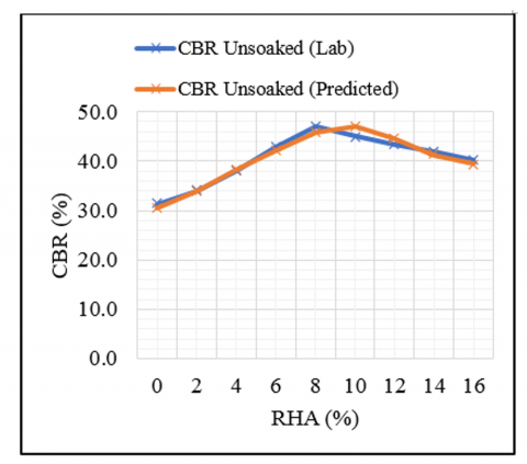
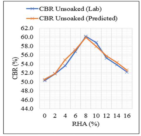
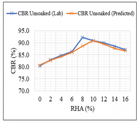
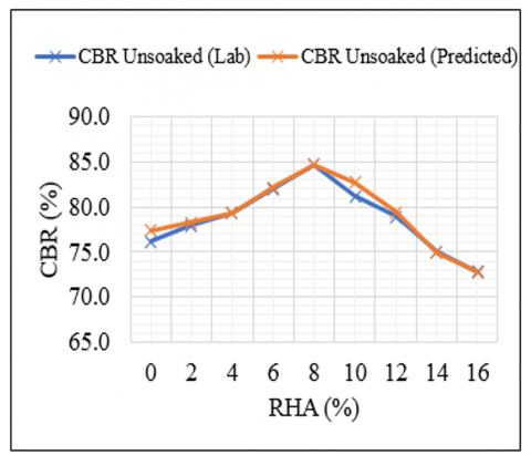
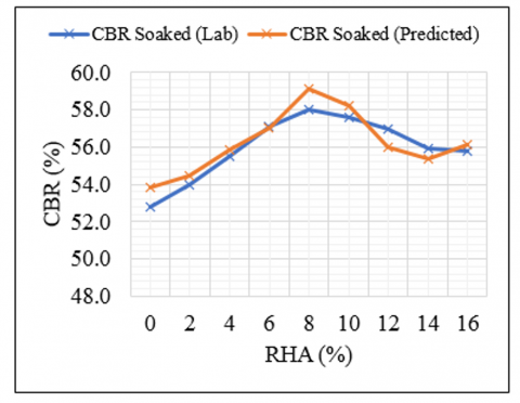
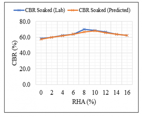
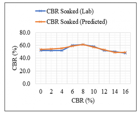
Artificial Neural Network (ANN) Results in Table 2 shows the details of the components of the ANN model. The six input variables were cement (%), rice husk ash (RHA) (%), optimum moisture content (%), liquid limit (LL) (%), plasticity index (PI) (%), and maximum dry density (MDD) (Kg/m3), while CBR Unsoaked (%) and CBR Soaked (%) were the two output variables. One hidden layer with ten layers of neurons. Figures 2 to 15 show the testing results of the observed (laboratory test results) and ANN predicted values of unsoaked and soaked CBR of natural soils (A-7-6) and cement-treated soils stabilized with rice husk ash. These values clearly signify the high precision and accuracy of the ANN models. Figure 2 shows the comparison between the observed (in the lab) and predicted unsoaked CBR values of A-7-6+RHA+0% cement. Figure 3 presents the comparison between the observed (in the lab) and predicted unsoaked CBR values of A-7-6+RHA+2% cement. Figure 4 depicts the comparison between the observed (lab) and predicted unsoaked CBR values of A-7-6+RHA+4% cement. Figure 5 shows the comparison between the observed (lab) and predicted unsoaked CBR values of A-7-6 +RHA+6% cement. Figure 6 gives the comparison between the observed (in the lab) and predicted unsoaked CBR values of A-7-6+RHA+8% cement. Figure 7 shows the comparison between the observed (in the lab) and predicted unsoaked CBR values of A-7-6+RHA+10% cement. Figure 8 presents the comparison between the observed (in the lab) and predicted unsoaked CBR values of A-7-6+RHA+12% cement. Figure 9 depicts the comparison between the observed (lab) and predicted soaked CBR values of A-7-6+RHA+0% cement, and Figure 10 shows the comparison between the observed (lab) and predicted soaked CBR values of A-7-6+RHA+2% cement. Figure 11 shows the comparison between the observed (lab) and predicted soaked CBR values of A-7-6+RHA+4% cement, and Figure 12 shows a comparison between the observed (lab) and predicted soaked CBR values of A-7-6+RHA+6% cement. However, Figure 13 depicts the comparison between the observed (lab) and predicted soaked CBR values of A-7-6+RHA+8% cement. and Figure 14 depicts a comparison between the observed (lab) and predicted soaked CBR values of A-7-6+RHA+10% cement. Figure 15 presents a comparison between the observed (lab) and predicted soaked CBR values of A-7-6+RHA+12% cement.
Table 2. Details of components of the ANN model
|
Number of inputs 6 Number of outputs 2 Number of hidden layer neurons 10 Number of output layer neurons 2 Number of epochs 21 |
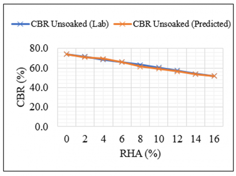
Figure 2. Comparison between observed (lab) and predicted unsoaked CBR values of A-7-6+RHA+0% cement
Figure 3. Comparison between observed (lab) and predicted unsoaked CBR values of A-7-6+RHA+2% cement
Figure 4. Comparison between observed (lab) and predicted unsoaked CBR values of A-7-6+RHA+4% cement
Figure 5. Comparison between observed (lab) and predicted unsoaked CBR values of A-7-6+RHA+6% cement
Figure 6. Comparison between observed (lab) and predicted unsoaked CBR values of A-7-6+RHA+8% cement
Figure 7. Comparison between observed (lab) and predicted unsoaked CBR values of A-7-6+RHA+10% cement
Figure 8. Comparison between observed (lab) and predicted unsoaked CBR values of A-7-6+RHA+12% cement
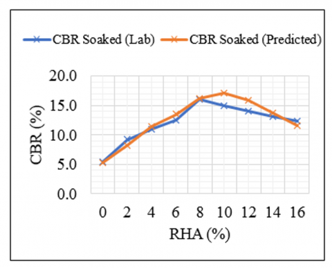
Figure 9. Comparison between observed (lab) and predicted soaked CBR values of A-7-6+RHA+0% cement
Figure 10. Comparison between observed (lab) and predicted soaked CBR values of A-7-6+RHA+2% cement
Figure 11. Comparison between observed (lab) and predicted soaked CBR values of A-7-6+RHA+4% cement
Figure 12. Comparison between observed (lab) and predicted soaked CBR values of A-7-6+RHA+6% cement
Figure 13. Comparison between observed (lab) and predicted soaked CBR values of A-7-6+RHA+8% cement
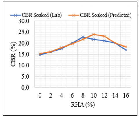
Figure 14. Comparison between observed (lab) and predicted soaked CBR values of A-7-6+RHA+10% cement
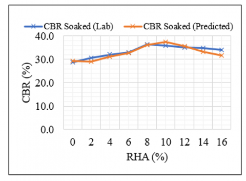
Figure 15. Comparison between observed (lab) and predicted soaked CBR values of A-7-6+RHA+12% cement
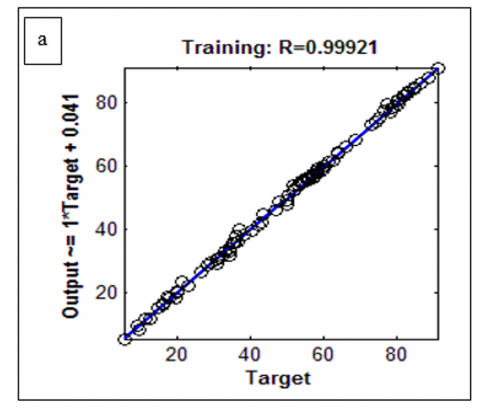
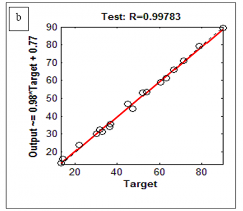
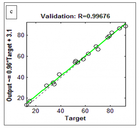
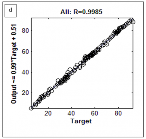
Figure 16. The regression plot showing the predicted (output) and target (observed) values for (a) Training dataset, (b) Testing, (c) Validation dataset, and (d) The prediction analysis of all the process during of the ANN model (RHA and A-7-6 and cement)
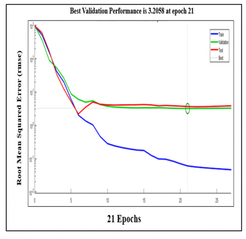
Figure 17. ANN prediction best validation performance
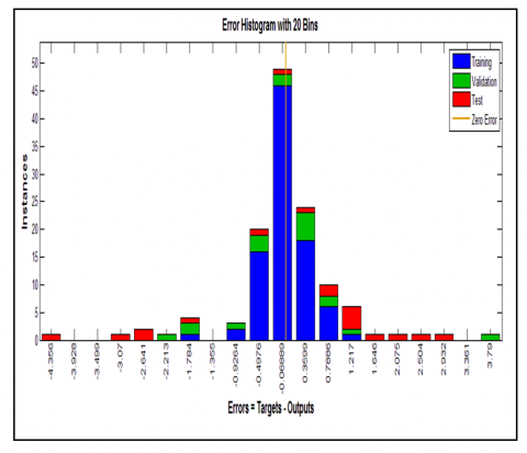
Figure 18. The ANN error plot for rice husk Ash at A-7-6 soil and cement
3.1 Regression plots for ANN modelling results for rice husk ash and A-7-6 soil
Figures 16(a-d) show the regression plot between observed and predicted CBR values of the A-7-6 soil stabilized with RHA and cement. Figure 16a shows the predicted (output) and target (observed) values for training dataset during training stage of ANN model. Figure 16b shows the predicted and target values for testing dataset during testing stage of ANN model. Figure 16c and Figure 16d shows the predicted (output) and target (observed) values for validating dataset during validating stage of ANN model. Performance of the neural network as indicated by coefficient of correlation (R2) at training, testing and validation and all prediction stages were; 0.99921, 0.9983, 0.99676 and 0.9985, respectively. According to Ebid [29], If R 0.8, there is a significant connection between two sets of variables. Since the model's R-value is 0.99, it can accurately determine CBR values. The prediction carried out by the ANN is viable and when applied it will give a significant optimal process for the application of lateritic soil admixed with cement and rice husk ash. This study is support by the work done by Harini and Naagesh [30].
Figure 17 displays the results of the training. The training stops after six consecutive increases in the validation error, and the best result is taken from the epoch with the least validation error. In overall, the error decreases as more training epochs are completed, but it may start to increase on the validation data set as the network starts struggling to maintain the training data in the activated form He et al. [31]. Figure 18 depicts the error plot of the prediction analysis via the ANN model.
This research studies the effects of rice husk ash on cement treated lateritic soil and makes efforts to develop a predictive model for CBR through the use of artificial neural network (ANN). This study clearly distinguishes itself not only by developing an ANN predictive model for CBR when soil is stabilized with cement, a common soil stabilizer, but the efficient management of a ubiquitous waste-rice husk, which upon being burnt under controlled conditions result to ash with pozzolanic properties that suitably complement cement, hence, reducing costs of road construction. The ANN models constitute a database of results of laboratory tests. ANNs is presented as a multi-layer perception and trained with feedback propagation algorithm, with the model input variables as: cement (%), rice husk ash (%), liquid limit (%), plasticity index (%), maximum dry density (MDD) (kg/m3) and optimum moisture content (%) with California bearing ratio (CBR) (both at soaked and unsoaked states) as the output. It is established that the chosen optimal model, with one single hidden layer of ten hidden layer neurons, is able to predict the CBR outcomes. The resultant optimal ANN shows sound accuracy with R of 0.99 and RMSE of 0.99, when validated against a set of unseen data. It can be concluded that the model can be recommended as a reliable tool to predict values of soaked and unsoaked CBR of cement treated laterites stabilised with rice husk ash (RHA), which upon optimal use would alleviate the monotony, time-wasting, costly-in terms of manpower and resources, processes of carrying out the CBR tests in the laboratory.
[1] Přikryl, R. (2021). Geomaterials as construction aggregates: a state-of-the art. Bulletin of Engineering Geology and the Environment, 80: 8831-8845. https://doi.org/10.1007/s10064-021-02488-9
[2] Trong, D.K., Pham, B.T., Jalal, F.E., Iqbal, M., Roussis, P.C., Mamou, A., Ferentinou, M., Vu, D.Q., Dam, N.D., Tran, Q.A., Asteris, P.G. (2021). On random subspace optimization-based hybrid computing models predicting the California bearing ratio of soils. Materials, 14(21): 6516. https://doi.org/10.3390/ma14216516
[3] Yildirim, B., Gunaydin, O. (2011). Estimation of California bearing ratio by using soft computing systems. Expert Systems with Applications, 38(5): 6381-6391. https://doi.org/10.1016/j.eswa.2010.12.054
[4] Bardhan, A., Gokceoglu, C., Burman, A., Samui, P., Asteris, P.G. (2021). Efficient computational techniques for predicting the California bearing ratio of soil in soaked conditions. Engineering Geology, 291: 106239. https://doi.org/10.1016/j.enggeo.2021.106239
[5] Ho, L.S., Tran, V.Q. (2022). Machine learning approach for predicting and evaluating California bearing ratio of stabilized soil containing industrial waste. Journal of Cleaner Production, 370: 133587. https://doi.org/10.1016/j.jclepro.2022.133587
[6] Selçuk, L., Şeker, V. (2019). Predicting California bearing ratio of foundation soil using ultrasonic pulse velocity. Proceedings of the Institution of Civil Engineers-Geotechnical Engineering, 172(4): 320-330. https://doi.org/10.1680/jgeen.18.00053
[7] Bardhan, A., Gokceoglu, C., Burman, A., Samui, P., Asteris, P.G. (2021). Efficient computational techniques for predicting the California bearing ratio of soil in soaked conditions. Engineering Geology, 291: 106239. https://doi.org/10.1016/j.enggeo.2021.106239.
[8] Katte, V.Y., Mfoyet, S.M., Manefouet, B., Wouatong, A. S.L., Bezeng, L.A. (2019). Correlation of California bearing ratio (CBR) value with soil properties of road subgrade soil. Geotechnical and Geological Engineering, 37: 217-234. https://doi.org/10.1007/s10706-018-0604-x
[9] Othman, K., Abdelwahab, H. (2023). The application of deep neural networks for the prediction of California Bearing Ratio of road subgrade soil. Ain Shams Engineering Journal, 14(7): 101988. https://doi.org/10.1016/j.asej.2022.101988
[10] Haupt, F.J., Netterberg, F. (2021). Prediction of California bearing ratio and compaction characteristics of Transvaal soils from indicator properties. Journal of the South African Institution of Civil Engineering, 63(2): 47-56. https://doi.org/10.17159/2309-8775/2021/v63n2a6
[11] Khasawneh, M.A., Al-Akhrass, H.I., Rabab’ah, S.R., Al-sugaier, A.O. (2022). Prediction of California bearing ratio using soil index properties by regression and machine-learning techniques. International Journal of Pavement Research and Technology, 1-19. https://doi.org/10.1007/s42947-022-00237-z
[12] Kurnaz, T.F., Kaya, Y. (2019). Prediction of the California bearing ratio (CBR) of compacted soils by using GMDH-type neural network. The European Physical Journal Plus, 134(7): 326. https://doi.org//10.1140/epjp/i2019-12692-0
[13] Hassan, J., Alshameri, B., Iqbal, F. (2021). Prediction of California bearing ratio (CBR) using index soil properties and compaction parameters of low plastic fine-grained soil. Transportation Infrastructure Geotechnology, 1-13. https://doi.org/10.1007/s40515-021-00197-0
[14] Bakri, M., Aldhari, I., Alfawzan, M. S. (2022). Prediction of California bearing ratio of granular soil by multivariate regression and gene expression programming. Advances in Civil Engineering, 2022. https://doi.org/10.1155/2022/7426962
[15] Gül, Y., Çayir, H.M. (2021). Prediction of the California bearing ratio from some field measurements of soils. In Proceedings of the Institution of Civil Engineers-Municipal Engineer, 174(4): 241-250. Thomas Telford Ltd. https://doi.org/10.1680/jmuen.19.00020
[16] Varol, T., Ozel, H.B., Ertugrul, M., Emir, T., Tunay, M., Cetin, M., Sevik, H. (2021). Prediction of soil-bearing capacity on forest roads by statistical approaches. Environmental Monitoring and Assessment, 193: 1-13. https://doi.org/10.1007/s10661-021-09335-0
[17] Abiodun, O.I., Jantan, A., Omolara, A.E., Dada, K.V., Mohamed, N.A., Arshad, H. (2018). State-of-the-art in artificial neural network applications: A survey. Heliyon, 4(11): e00938. https://doi.org/10.1016/j.heliyon.2018.e00938
[18] Dongare, A.D., Kharde, R.R., Kachare, A.D. (2012). Introduction to artificial neural network. International Journal of Engineering and Innovative Technology (IJEIT), 2(1): 189-194.
[19] da Silva, I.N., Spatti, D.H., Flauzino, R.A., Liboni, L.H.B., dos Reis Alves, S. F. (2017). Artificial neural networks: A practical course. Springer Cham. ISBN (Softcover). 978-3-319-82751-3. https://doi.org/10.1007/978-3-319-43162-8
[20] Chao, Z., Ma, G., Zhang, Y., Zhu, Y., Hu, H. (2018). The application of artificial neural network in geotechnical engineering. In IOP Conference Series: Earth and Environmental Science, 189(2): 022054. IOP Publishing. https://doi.org/10.1088/1755-1315/189/2/022054
[21] Moayedi, H., Mosallanezhad, M., Rashid, A.S.A., Jusoh, W.A.W., Muazu, M.A. (2020). A systematic review and meta-analysis of artificial neural network application in geotechnical engineering: theory and applications. Neural Computing and Applications, 32: 495-518. https://doi.org/10.1007/s00521-019-04109-9
[22] Yin, Z.Y., Jin, Y.F., Liu, Z.Q. (2020). Practice of artificial intelligence in geotechnical engineering. Journal of Zhejiang University-Science A: Applied Physics & Engineering, 21(6): 407-411. https://doi.org/10.1631/jzus.A20AIGE1
[23] Zhang, W., Li, H., Li, Y., Liu, H., Chen, Y., Ding, X. (2021). Application of deep learning algorithms in geotechnical engineering: A short critical review. Artificial Intelligence Review, 54(8): 5633-5673. https://doi.org/10.1007/s10462-021-09967-1
[24] Ly, H.B., Le, T.T., Vu, H.L.T., Tran, V.Q., Le, L.M., Pham, B.T. (2020). Computational hybrid machine learning based prediction of shear capacity for steel fiber reinforced concrete beams. Sustainability, 12(7): 2709. https://doi.org/10.3390/su12072709
[25] Onyelowe, K.C., Ebid, A.M., Nwobia, L.I., Obianyo, I. I. (2022). Shrinkage limit multi-AI-based predictive models for sustainable utilization of activated rice husk ash for treating expansive pavement subgrade. Transportation Infrastructure Geotechnology, 9(6): 835-853. https://doi.org/10.1007/s40515-021-00199-y
[26] Taleb Bahmed, I., Harichane, K., Ghrici, M., Boukhatem, B., Rebouh, R., Gadouri, H. (2019). Prediction of geotechnical properties of clayey soils stabilised with lime using artificial neural networks (ANNs). International Journal of Geotechnical Engineering, 13(2): 191-203. https://doi.org/10.1080/19386362.2017.1329966
[27] Nowland, S.J., Hinton, G.E. (1995). Simplifying neural networks by weight sharing. Neural Computation, 4(4): 473-493. https://doi.org/10.1162/neco.1992.4.4.473
[28] Li, L., Luo, Z., He, F., Sun, K., Yan, X. (2022). An improved partial similitude method for dynamic characteristic of rotor systems based on Levenberg–Marquardt method. Mechanical Systems and Signal Processing, 165: 108405. https://doi.org/10.1016/j.ymssp.2021.108405
[29] Ebid, A.M. (2021). 35 Years of (AI) in geotechnical engineering: state of the art. Geotechnical and Geological Engineering, 39(2): 637-690. https://doi.org/10.1007/s10706-020-01536-7
[30] Harini, H., Naagesh, S. (2014). Predicting CBR of fine-grained soils by artificial neural network and multiplelinear regression. International Journal of Civil Engineering and Technology (IJCIET), 5(2): 119-126.
[31] He, K., Zhang, X., Ren, S., Sun, J. (2015). Spatial pyramid pooling in deep convolutional networks for visual recognition. IEEE Transactions on Pattern Analysis and Machine Intelligence, 37(9): 1904-1916. https://doi.org/10.1109/TPAMI.2015.2389824