ShreeNandhini Parthiban* | Palaniswamy Amudha| Subramaniam Pillai Sivakumari
© 2022 IIETA. This article is published by IIETA and is licensed under the CC BY 4.0 license (http://creativecommons.org/licenses/by/4.0/).
OPEN ACCESS
Air pollution is a major issue because Particulate Matter (PM) has a substantially higher effect on human health than other pollutants. Air Quality (AQ) prediction has become critical recently to take action to reduce pollution. This research introduces a unique methodology for assessing the effectiveness of PM10 and PM2.5. Enhanced spatial, temporal sequence-Improved Sparse Auto Encoder with Deep Learning (EISAE-DL) has been proposed to predict AQ affected by the prolonged dependency of air pollution congregation. However, Long Short-Term Memory (LSTM) used in EISAE-DL has suffered from the learning of a long-term dependent sequence of the training dataset. In addition, it is hard to create very reliable AQ forecasts at higher periodic frequencies, such as daily, weekly, or even monthly. This paper proposes Transfer learning (TL) in a Stacked Bidirectional and Unidirectional LSTM to solve the learning issue in LSTM for long-term dependencies. So, EISAE-DL with TL and modified LSTM model is named as EISAE-Deep Transfer Learning (EISAE-DTL). TL with a modified structure can handle large-size datasets effectively. However, training time is increased more than twice for non-transfer learning way of modeling due to TL, Wasserstein Distance-based adversarial learning is proposed in EISAE-DTL to decrease the variances among AQ data collected from any two sites. The proposed work is named EISAE- Enhanced DTL (EISAE-EDTL). The developed EISAE-DTL and EISAE-EDTL models are compared and analyzed with the performance of existing algorithms EISAE-DL, ISAE-DL, TL-BLSTM, MMSL, and ST-DNN. The experimental findings demonstrate the accuracy, precision, sensitivity, specificity, Area Under Curve (AUC), and Matthew's correlation coefficient of the proposed model performs admirably and improves present condition approaches.
air quality prediction, deep learning, deep transfer learning, improved sparse auto encoder, feature modeling, stacked bidirectional and unidirectional LSTM
As AQ deterioration is becoming more of an issue, Particulate Matter (PM) has a considerable negative influence on human well-being. Since the fine PM2.5 has a smaller diameter, it can reach the alveoli and even the bronchioles more quickly, interrupting lung gas interchange. Long-term submission of PM in the air raised the risk of cardiovascular illness, respiratory problems, and lung cancer [1, 2]. AQ monitoring systems have been set up in various localities in response to rising public health awareness. On the other hand, several providers merely can expose the AQ and cannot predict it. Predicting AQ is critical for directing choices and actions aimed at minimizing PM2.5 prominence, such as evaluating whether to participate in internal or external activities. Consequently, a complicated array of elements [3, 4] such as emissions, traffic conditions, and weather data, make precise AQ prediction challenging.
In the lack of physical models, data mining enables novel approaches for analyzing AQ [5, 6] and may find hidden patterns in the acquired data. A Machine Learning (ML) based method was developed [7] that considered both spatial and regional relationships into account. The spatial classifier Artificial Neural Network (ANN) analyzes global information by utilizing mean results gathered from the surrounding regions. However, the results of this model were unaffected by local and global climatic conditions.
The three-input regression model was proposed to combine temporal and spatial predictors with regional weather information [8]. The identification features may vary to the urban scenario an extraordinary increase in people activity, and higher electricity and transport requirements. These elements play a key role in urban air pollution caused by clogged major highway networks. A linear model approach considers these factors [9].
The more factors considered for AQ prediction make decisions more precise. Also, knowledge obtained from huge datasets improves the accuracy of AQ prediction. So, DL models [10, 11] were used for AQ prediction. But, all proposed AQ prediction models suffered from data dissimilarity of collected data from various cities. Also, they cannot handle long delay-based dataset, which causes a high learning time.
So, the data dissimilarity issues were solved in ISAE-DL and EISAE-DL techniques using an auto-encoder and DL method [12]. The data collected from spatially and temporally correlated locations are grouped based on Manhattan distance. The PM-related data are fed into ANN and LSTM while topography data are fed into CNN. Then, aggregated data is fed into a sparse autoencoder for normalization. Then classifier is used for AQ prediction. The LSTM used in EISAE-DL is suffered to learn the long-term dependencies of air pollutant concentrations. The learning issue in LSTM for long-term dependencies is solved in this paper by using Transferred Stacked Bidirectional and Unidirectional LSTM-based transfer learning in EISAE-DL which handle large size and long delay-dependent datasets. Wasserstein Distance-based DTL (WD-DTL) is employed in EISAE-DTL to minimize the disparities across the origin and destination areas through adversarial learning. In summary, the major contribution of this paper is the following:
The remaining sections of the manuscript are structured as follows: Section 2 discusses the literature on the diagnosis of DL-based AQ prediction. Proposed EISAE-DTL and EISAE-EDTL are described in Section 3 and the results are shown in Section 4. The study is summed up and suggestions for further research are offered in Section 5.
An Apriori pattern mining technique [13] was employed to mine contextual spatial-temporal correlations among PMs. The temporal sequences provide high-frequency rule generation from specified intervals in each time series. Thus the techniques emerge to identify the relationship among emissions in various locations with varying timeframes. On the other hand, periodically executing the rule creation process for every data update is a time-consuming process.
As a means of improving the accuracy of the nonlinear AQ Index (AQI) series, a novel hybrid learning strategy [14] was provided with multidimensional scaling-based K-means and a Modified Extreme Learning Machine (MELM) for urban AQ prediction. Predictions for AQ were made using a neuro-fuzzy network and self-organizing clustering [15]. To fine-tune the network's settings, evolutionary techniques like steepest descent backpropagation are employed. Fuzzy rules, once learned, can be utilized to make predictions about the AQ of test data.
However, ML-based approaches are limited to processing large-size datasets. To solve this issue, DL-based approaches were proposed to handle large-size data efficiently. A Spatial-Temporal Deep Neural Network (ST-DNN) was a comprehensive predictive model [16] for AQ forecasts by incorporating data from a wide range of monitoring sites, temperature, wind features, and direction and elevation information. A temporal sliding-based Bidirectional LSTM (BLSTM) with which strong temporal connections can be preserved [17] was proposed to handle PMs and related information integrated with an appropriate time lag. AQ forecasting using a TL-BLSTM [18] was proposed which learns from PM2.5's long-term dependencies and then uses transfer learning to apply that knowledge across different time scales.
Empirical Mode Decomposition (EMD) and BLSTM were proposed [19] that consist solely of PM2.5 time-series data, which are treated as signal data. To break down the data and pull out the frequency and amplitude features, EMD is used as an unsupervised feature learning method. AQ prediction of shorter-term trends, especially for unexpected shifts, was enhanced by this method. Multi-output and Multi-index of Supervised Learning (MMSL) were developed in LSTM [20] to simultaneously learn the PM data of the current monitoring station and its nearest neighbor stations.
The underlying uncertainties associated with data necessary to run these models are another source of uncertainty in operational models. The natural sources associated, for instance, are hard to fully characterize. The disadvantages of operational models involve the usage of standard settings and the lack of information for the same geographical scale that might be used to evaluate model findings. To solve these issues, a novel AQ prediction technique is proposed in this paper.
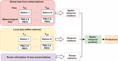
This model considers the Air quality data in India (2015 – 2020) database, which comprises the name of the city, date, PM2.5, PM10, NO, NO2, NOx, NH3, CO, SO2, O3, Benzene, Toluene, Xylene, AQI, and class of different stations across 26 places in India. It is retreived from kaggle website. The suggested predictive model framework, depicted in Figure 1, is made up of four key components. TG refers global time between all datations. TL represent the local time history of data colelcted in every stations.Time perid is 3 years durarion from every day with every 6 hours colelctions.
Figure 1. Overall prediction framework
To examine the sequence delays and linkages among places using past temporal patterns, as well as to analyze location feature variations for future determinants, to uncover the most significant interactions between locations. Even if they have substantial correlations with the target place, it is worthwhile to investigate nearby places. ISAE-DL and EISAE-DL connection extractors are used to find the most comparable locations to the requested location, and then create training datasets from the best $k$ associated locations. At last, the prediction outcomes of the DL model must be trained and tested.
The suggested EISAE-DTL paradigm combines objective location temporal data, related position spatial-temporal data, and terrain data. The data stream contains statistical data from the target and related sites, such as pollution levels, weather conditions, and objective features, as well as changes over a previous couple of hours. These data are given as input to LSTM, Adaptive Temporal Extractor (ASE), and ANN. This information was fed into the LSTM and ANN. A matrix of 121 squares was employed for topography data, equivalent to 1111 reference locations at 500 m intervals, with the principal square in the matrix reflecting the present areas. As a result, there are 120 previously unknown locations with AQI estimated using WD-based deep adversarial TL.
Concatenating the proportional altitude with the unknown points AQIs and these points are given as input to the CNN to lessen AQI influence at a greater altitude. CNN inputs can be fine-tuned later to improve accuracy. Contaminants, climatic situations, and objective attribute(s) of regions with significant resemblance (identified by ISAE-DL and EISAE-DL) were entered into the EISAE-DL and ASE without any previous training. To integrate TRE, SRE, and TE, a two-layer Feed-forwrad FNN was used. The divergence among the targeted feature value and a particular time $t_{q+h}$ where $t_{q+h}<f i_t$ was the actual prediction.
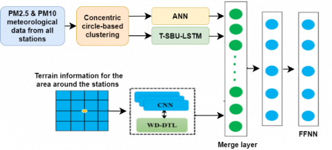
Figure 2. Architecture of EISAE-DTL framework
The model's structure is depicted in Figure 2. EISAE-DL and ASE receive data on AQ and meteorological conditions, whereas CNN receives data on terrain [21]. The models are con catenated beside each other, and the parameters are transferred onto the next layer. Because the present state evolves in terms of its impact on upcoming time intervals, the classifier is constructed hourly throughout the next 48 hours.
As a result, in specified time intervals, the inputs are integrated with the desired feature changes to learn distinct versions with identical topologies multiple times. This approach has the advantage of maintaining uniform input sizes regardless of position or time. To extract AQ feature information from linked sites identified by ISAE-DL and EISAE-DL, the spatial-temporal relationships extractor (SRE) utilizes an ANN model The temporal relationships extractor (TRE) collects AQ attributes using meteorological data obtained in the objective region during the last few hours to apply an LSTM model.
3.1 Temporal relations
The temporal sequence input for PM2.5, PM10, and other elements are continuous and constant, and they can be classified as lower (trends) or high (fast growth) bandwidth data. EISAE-DTL is developed to acquire target location time series patterns because EISAE-DL simulates historical time series behavior; however, the ANN employs only recent data and is thus sensitive to quick changes. As a result, the EISAE- DL, and ANN obtain less and more bandwidth data from the patterns, respectively. The EISAE-DTL forecasts trends in PM2.5 and PM10 levels for the last six hours and local weather parameters (wind speed and direction, humidity, and temperature), whereas the ASE TRE enhances model sensitivity by utilizing similar attributes as the EISAE-DTL. Preceding research work has established the significance of these features in terms of AQ [22].
3.2 Spatial-temporal relations
Contaminant diffusion refers to the ability to link AQ at one area with that at other locations Because AQ in a single area is influenced by both local pollutants and pollution from neighboring locations, SRE takes into account past spatial-temporal nearby location features as inputs.
As a result, SRE is developed which leverages AQIs and meteorological data from other places to calculate AQ at the target location. Terrain factors, such as a hilltop between locations, are underestimated when partitioning spaces into sections using circles of varying diameters. Data from partitioned regions is frequently comprised of mean or mode values, which are incredibly unreliable, especially in areas with few locations. Furthermore, for an SRE position, data mining from places in the spatial-temporal proximity using ISAE-DL and EISAE-DL is required, which includes AQIs and meteorological variables (wind speed and direction) for the previous 6 hours. The spatial-temporal neighborhood period sequences such as the target location are undeniably durable and coherent. As a result, by accounting for spatial-temporal neighborhood influences, ANN-SRE is used to improve model stability [22].
3.3 Terrain extractor
Due to various barriers and elevation variances, the relationships between locations differ. As a result, most terrain information is utilized to improve position associations. Terrian is generally expressed in terms of the elevation, slope, and orientation of the area around the stations. Terrain statistics in the locations were obtained using a 121-square-section vector made up of 11*11 coordinate lines spaced 500 meters apart. To establish the correlations between terrain and PM2.5 & PM10, the approach [23] of is used for the evaluation of each location is normalized as Eq. (1):
$E l_s=\frac{e l e-e l e_{s t}}{e l e_{s t}}$ (1)
and transferred to equivalent altitude is expressed as Eq. (2):
$e l e_{r e l}=\frac{1}{e^{E l_S}}$ (2)
The standardized altitude is represented as$E l_s$, and it reduces the effect of higher altitudes, although the distribution is heavily sensitive to elevation. The TE, SRE, and TRE results are combined and given to the FFNN using an enhanced sparse autoencoder. Figure 2 depicts the suggested approach's general framework. The upgraded sparse autoencoder accomplishes the process of layer blending and outlier detection. The input data is successfully managed in a systematic manner.
Complex forms are formulated from smaller shapes with the use of an autoencoder. Autoencoders are capable and efficient detectors of important features. For the learning experience, data is combined in both continuous and categorical forms. The value obtained is multiplied by the input data in this strategy, which employs a feed-forward artificial neural network-based perceptron. The linear function, log-sigmoid, hard limit, and hyperbolic tangent with probable saturation is used to start the process, which is then added to the total inputs and weights. The value of the consequence is calculated as Eq. (3):
$B=f(w p+a)$ (3)
In Eq. (3), f(∙) is the activation function, $w$ is the weight value, $a$ is the bias, and $p$ is the given input. Traditionally, perceptrons employ a primary function for prediction, and the commonly chosen function is provided by Eq. (4)
$f(p)=\frac{1}{\left(1+e^{-x}\right)}$ (4)
The precise estimation of the weight lowers the error among the output and the assumed value is decided in the training set of data. The existence of multiple perceptrons is organized as several layers, with each layer's output data being sent to the input of the next layer. This multilayer network can solve challenging linear separable classification problems. By using the initial weights, the input data is propagated [24]. The error value can be estimated from the desired outcome, which is the variance in feed-forward propagation output. The algorithm is developed in batches, and each test is completed before the weight is updated. The mean of the elevation value is used to optimize the weights, and each input is probed by the revised weights, while the output data is categorized correspondingly.
3.4 Proposed EISAE-DTL
The proposed Enriched spatial, temporal sequence-Improved Sparse Auto Encoder with Deep TL (EISAE-DTL) algorithm is mainly used to solve the learning issue in LSTM for long-term dependencies. Deep LSTM frameworks are networks with several stacked LSTM hidden layers, with each LSTM hidden layer's output passing into the next LSTM hidden layer. To enhance prediction accuracy at higher temporal resolutions, TL is used. To transmit data from the source to the new domain, TL exploits similarities between two separate datasets, tasks, or models.
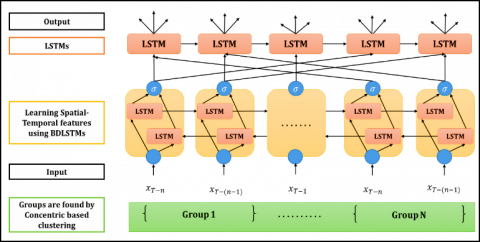
Figure 3. Architecture of T-SBU-LSTM
This research adopts the stacked-layers technique, which has been found to improve neural network efficiency. T-SBU-LSTM was used in EISAE-DL to forecast network-wide traffic speed values. Figure 3 depicts the T-SBU-LSTM design. The Transferred Stacked Bidirectional and Unidirectional LSTM (T-SBU-LSTM) is proposed as a method for learning from long-term PM2.5 dependencies in this study, and it employs TL to deliver data from lower to higher temporal resolutions. Figure 3 depicts the T-SBU-LSTM structure.
BLSTM is an improved RNN that can learn long-term dependencies from both upwards and backward sequences of time series data. SBU-LSTM (Stacked Bidirectional and Unidirectional LSTM) is an AQ prediction model developed by merging LSTM and BLSTM. The proposed paradigm can deal with both long-term and short-term dependency. This phase of research extends the AQ prediction from a single place to multiple nearby locations, with time delays ranging from short to lengthy. By learning both forward and backward dependencies, the integrated architecture improves feature learning from large-scale spatiotemporal time series data.
TL allows the model to learn and store information from samples with lower temporal resolutions, as well as increase prediction performance for data with higher temporal resolutions. The initial feature-learning layer of T-SBU-LSTM is a BLSTM layer, while the last layer is an LSTM layer. The T-SBU-LSTM can be filled with one or more LSTM/BLSTM layers in the middle to make full use of the input data and learn sophisticated and extensive features. T-SBU-LSTM predicts future temporal values for one time step using spatial time series data as input. Based on past data, the SBU-LSTM can also estimate values for numerous future time steps.
Initially, the sequences are projected for the targeted area using time sequence attributes that incorporate spatial data after selecting the places with the greatest significant spatialtemporal linkages to the specified area. Consequently, the position remains constant, but the time series might change depending on where they are. A mountain between two points, for example, could affect the sequences. As a result, the prediction model takes into account both time and spatial relationships. To extract features for prediction, the spatial and temporal connection features should be developed. Assume, the group of regions: $A=\{a 1, a 2, \ldots a n\}$ and set of features: $F S=\{f s 1, f s 2, \ldots . f s m\}$. Although each area contains geographical data like latitude and longitude, the area coordinate (AC) is described as Eq. (5):
$A C_i=\left(a_i, l_i, m_i\right) a_i \in A$ (5)
The latitude and longitude of area ai are li and mi, respectively. Considering related geographical features may enhance prediction, the distance between two locations is computed as Eq. (6):
$D_{p, q}=$ dist $_{\text {area }}\left(A C_p, A C_q\right)=$dist $_{\text {area }}\left(\left(a_p, l_p m_p\right),\left(a_q, l_q m_q\right)\right), a_p, a_q \in A p \neq q$ (6)
To discover the spatial domain's closest strongly linked areas, and the Spatial Relationships Sequence Set (SRSS) as Eq. (7):
$S R S S=\left\{D_{1,2}, D_{1,3} \ldots \ldots D_{n-1, n}\right\}, D_{i, j}=0,0<i<n+1$ (7)
where, $n$ is the number of positions and the diagonal numbers $D_{i, j}$ will be 0.SRSS_cand $\left(a_i, x\right)$ is a set of $x$ regions with the shortest spatial proximity to $a_i$.To investigate the attributes of these major spatial places, as areas with identical pattern sequences may aid prediction. The Feature Sequence Interval (FSI) for a particular region is described as Eq. (8):
$F\left(a_i, f s_j, t_{v t, s t}=\left\{b\left(a_i, f s_j, t_{v t}\right), b\left(a_i, f s_i, t_{v t+1}\right)\right.\right., \left.\left.b\left(a_i, f s_i, t_{v t}\right), a_i \in A, f s_j \in F S, v_t<s_t\right\}\right)$ (8)
where, $a_i$ has a variable feature $f s_i$ from start to end $\left(v_t\right.$ to $S_t$ time $\left(v_t<s_t\right)$, and $\mathrm{b}\left(a_i, f s_j, t_x\right)$ indicates the observed level of off $f s_j$ at $t_x$. For any two sites, the proximity across feature patterns can be represented as Eq. (9):
$D S_{p, q, t_{v t, s t}}=\operatorname{dist}_{\text {seq }}\left(F\left(a_p, f s_{\text {target }}, t_{v_t, s_t}\right), F\left(a_q, f s_{\text {target }}, t_{v_t, s_t}\right)\right)a_p, a_q \in A, \quad p \neq q$ (9)
Apply TL to enhance the performance of the prediction model. Assume a target training set of $\mathrm{n}_{\mathrm{t}}$ instances $A q_t$ = $\left\{\left(a_1^t, b_1^t\right), \ldots \ldots,\left(a_{n_t}^t, b_{n_t}^t\right)\right\}$ drawn from some probability $D_i$, and an origin learning set of ns samples $A q_s$ = $\left\{\left(a_1^t, b_1^t\right), \ldots \ldots,\left(a_{n_s,}^t, b_{n_s}^t\right)\right.$. The objective and source training sets maintain the identical feature space and label space, with each input feature vector $a i \in E n$ and the accompanying class label $b i \in\left\{C_1, \ldots, C_L\right\}$. Further, target data $A q_t$ should not be inferred from the same distribution as the source data $A q_s$, implying that the models derived from the source set would be unable to reliably identify the (target) test data due to the different time series. The size of $A q_t$, on the other hand, is typically insufficient for training an effective classifier for the test data. The purpose of TL is to use knowledge from $A q_s$ to aid in the learning of the target prediction function in $A q_t$.
In order to find the positions which are mostly related closely before utilizing the measures, initially, feature $\mathrm{fs}_{\text {target }}$ is selected to act as the objective detection sequence: in this case, PM2.5 was selected, but other objectives might be utilized if necessary. Eq. (10) can then be used to compute the collection of Temporal Relations Sequence Set (TRSS).
$T R S S_{t_{v t, s t}}=\left\{D S_{1,2, t_{v t, s t}}, \ldots \ldots \ldots D S_{n-1, n, t_{v t, s t}}\right\}$ (10)
The set of x positions with the minimum variations from position i is then chosen as TRSS_cand $\left(a_i, x\right)$. The Spatial-Temporal Relations (STR) cluster is introduced which is the collection of locations that are most strongly associated to $a_i$ To investigate both linkages respectively in Eq. (11)
STR_cand$\left(a_i, x\right)$=SRSS_cand$\left(a_i, x\right) \cup$
TRSS_cand $\left(a_i, x\right), \mathrm{a}_{\mathrm{i}} \in \mathrm{A}$ (11)
Instead of using the intersection, the union of SRCS cand $\left(a_i, x\right)$ and TRSS cand $\left(a_i, x\right)$ is used to provide a greater value of connections for the methodology to train; the conjunction will have lesser candidates (or none at all), leading to the in the absence of significant objective quality because certain location behaviors varied from adjacent locations. The Spatial-Temporal Predictor (STP) is defined by $S T R_{\text {cand }\left(a_i, x\right)}$ Eq. (12):
$P\left(\operatorname{STR}_{\text {cand }\left(a_i, x\right)}\right)\left[t_{t_l, t q}\right]=F\left(a_i, f s_{\text {target }}, t_{v t^{\prime}, s t^{\prime}}\right)$, $t_l<b_q<v t^{\prime} \leq s t^{\prime}$ (12)
In the above equation, $P$ predicts a series of objective qualities and delivers a sequential set, $S$ which provides the expected objective characteristics For the temporal range from tvt to tst,. $F$ is produced from the nearest identical time series, where tl is the recalled time when comparing tl to tq.
Algorithm 1: Pseudocode for EISAE-DTL
Input: Target Terminal (T); set of geographic coordinates (LC), number of candidates (n)
Output: Set of locations L
Step 1: Start the process
Step 2: Assume a set of areas: $A=\{a 1, a 2, \ldots a n\}$
Step 3: Assume a set of features: $F S=\{f s 1, f s 2, \ldots . f s m\}$
Step 4: Compute Area Coordinate (AC) $\mathrm{AC}_{\mathrm{i}}=\left(\mathrm{a}_{\mathrm{i}}, \mathrm{l}_{\mathrm{i}}, \mathrm{m}_{\mathrm{i}}\right)$
//Let latitude and longitude of area ai are li and mi
Step 5: Calculate the distance between two locations $D_{p, q}=$ dist $_{\text {area }}\left(A C_p, A C_q\right)=$ dist $_{\text {area }}\left(\left(a_p, l_p m_p\right),\left(a_q, l_q m_q\right)\right), a_p, a_q \in A$
//Apply TL for T-SBU-LSTM
Step 6: Initialize AQ data $\widetilde{\mathrm{Aq}}_{\mathrm{s}}=\varnothing$.
Step 7: for l = 1 to L do
7.1 Initialize a multilayer autoencoder MAEl (W,b).
7.2 Select location-based AQ Aqtc1 from Aqt.
7.3 Train AEl(W,b) using Aqtc1
7.4 Select location-based AQ Aqsc1 from Aqs
7.5 Reconstruct data $A q_s^{c_1}=\widetilde{M A} E_{\text {Recon }}^1\left(A q_s^{c_1}\right)$
7.6 Update the reconstructed data $\widetilde{A q}_{\mathrm{s}} \cup \mathrm{Aq}_{\mathrm{s}}^{\mathrm{c}_1}$
Step 8: end for
Step 9: Find spatial relationships sequence SRSS ={D1,2, D1,3, ….. Dn-1,n}, //Di,i= 0 // n is the integer spots, and the oblique values are Di,i, are 0.
Step 10: Compute FSI $F\left(a_i, f s_j, t_{v t, s t}=\left\{b\left(a_i, f s_j, t_{v t}\right), b\left(a_i, f s_i, t_{v t+1}\right), \ldots . b\left(a_i, f s_i, t_{v t}\right), a_i \in A, f s_j \in F S, v_t<s_t\right\}\right)$
// ai possesses fsi that fluctuates from start to end (vt to st) time (vtst); and b(ai,fsj,tx) indicates the measured fsi level at tx.
Step 11: Find the distance between feature sequences
Step 12: $D S_{p, q, t_{v t, s t}}=\operatorname{dist}_{\text {seq }}\left(F\left(a_p, f s_{\text {target }}, t_{v_t, s_t}\right), F\left(\begin{array}{c}a_q, f s_{\text {target, }} \\ t_{v_t, s_t}\end{array}\right)\right)$, $a_p, a_q \in A$
Step 13: Compute TRSS $T R S S_{t v t, s t}=\left\{D S_{1,2, t_{v t, s t}}, \ldots \ldots \ldots D S_{n-1, n, t_{v t, s t}}\right\}$
// The set of x positions with the minimum variance from position i is then chosen as TRSS_cand (ai,x).
Step 14: Evaluate STR STR_cand $\left(a_i, x\right)$ = SRSS_cand $\left(a_i, x\right) \cup$ TRSS_cand $\left(a_i, x\right)$
Step 15: Each location is normalized as $E l_s=\frac{e l e-e l e_{s t}}{e l e_{s t}}$
Step 16: Transferred to equivalent altitude is expressed as $e l e_{r e l}=\frac{1}{e^{E l_s}}$
Step 17: Calculate STP
P(STR_cand$\left(a_i, x\right)$)$\left[t_{t_l, t q}\right]=F\left(a_i, f s_{\text {target }}, t_{v t^{\prime}, s t^{\prime}}\right)$
Step 18: ASE receives data on AQ and meteorological conditions, whereas CNN receives data on terrain
Step 19: Concatenate each other and the parameters are transferred onto the next layer
Step 20: Perform a feedforward pass using FFNN
Step 21: Determine the activations for levels L2, L3, and so on, all the way up to the output layer Lnl.
Step 22: End the process
3.5 Proposed EISAE-EDTL
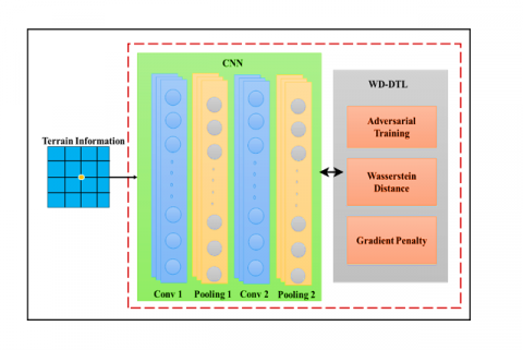
EISAE-EDTL is designed to shorten the training time of TL due to heavier data in the source domain by employing WD-DTL to optimize the differences among the actual and desired domains. Figure 4 depicts the WD-DTL architecture. The TL method is used to investigate the transferable characteristics of an AQ dataset under various meteorological situations. The atmospheric statistics are temperature, wind speed and direction, average wind speed and direction, humidity level, and elevation. Initially, a basic LSTM model is trained with appropriate data. Then, to acquire terrain features across source and target regions around the stations, the WD-DTL is developed and combined with the CNN, which minimizes the learning period. A neural network (known as domain critic) is built to calculate the actual Wasserstein proximity by improving domain critic loss. The LSTM-based feature extractor variables are then adjusted using a discriminator by lowering the predicted empirical Wasserstein distance. Using the adversarial training approach mentioned above, transferable attributes from a given area with confirmed erroneous labels can be used to diagnose a different yet similar detection objective without any tagged examples.
Figure 4. Architecture of CNN –WD-DTL
Suppose Aqs and Aqt are the objective datasets; the learning rate for classifier and feature learning is 2, whereas the training rate for domain conformity critic is 1. the batch size is $n$; the critic training step is $C t$, and the balance coefficients and fe are the first CNN-based feature extractor variable, cp is the preliminary domain alignment critic parameters, and pp is the initial detective variable Gradient distance is calculated as Eq. (13):
$\operatorname{ggrad} \leftarrow\left(\| \nabla_2 g_{\text {grad }} \leftarrow\left(\left\|\nabla_f p_c(f)\right\|_2-1\right)^2\right.$ (13)
The Wasserstein-1 distance can be approximated as:
$l i_{w d}=\frac{1}{N^s} \sum_{a^s \in A q^s} p_c\left(p_f\left(A q^s\right)\right)-\frac{1}{N^s} \sum_{b^t \in A q^t} p_c\left(p_f\left(A q^t\right)\right)$ (14)
Algorithm 2 Pseudocode for EISAE-EDTL
Input: Target Terminal (T); Set of geographic coordinate (LC), number of candidates (n)
Output: Set of locations (L)
Step 1: Start the process
Step 2: Assume a set of areas: A={a1,a2,…an}
Step 3: Assume set of features: FS = {fs1,fs2,…..fsm}
Step 4: Compute Area Coordinate (AC) ACi = (ai, li, mi) //Let latitude and longitude of area ai are li and mi
Step 5: Calculate the distance between two locations Dp,q = distarea (ACp, ACq) = distarea((ap,lp,mp), (aq,lq,mq))
Step 6: ASE receives data on AQ and meteorological conditions, whereas CNN receives data on terrain // Apply WD-DTL
Step 7: While θfe, θcp, and θ pp have not converged do
Step 8: Assume the source dataset $A q_t=\left\{\left(a_1^s, b_1^s\right)\right\}_{i=1}^n$
Step 9: Assume the target dataset $A q_s=\left\{a_1^t\right\}_{i=1}^n$
Step 10: For i=0,……Ct
Step 11: $f s \leftarrow p f(A q s), f t \leftarrow p f(A q t)$,
Step 12: $f \leftarrow\{f s, f t, f r\}$
Step 13: $g_{\text {grad }} \leftarrow\left(\| \nabla g_{g r a d} \leftarrow\left(\left\|\nabla_f p_c(f)\right\|_2-1\right)^2\right.$
$\theta_{c p} \leftarrow \theta_{c p}+\beta_1 \nabla \theta_{c p} l i_{w d}\left(a^s, b^t\right)-\tau g_{g r a d}(f)$
Step 14: end for
$\theta_{p p} \leftarrow \theta_{p p}+\beta_2 \nabla \theta_{p p} l_{c t}\left(a^s, b^s\right)$
$\theta_{f e} \leftarrow \theta_{f e}+\beta_2 \nabla \theta_{f e}\left[l_{c t}\left(a^s, b^s\right)+\delta l i_{w d}\left(A q^s, A q^t\right)\right]$
Step 15: end while
Step 16: Find spatial relationships sequence
SRSS ={D1,2,D1,3,…..Dn-1,n},//Di,i= 0 // n is the integer spots, and the oblique values are Di,i, are 0.
Step 17: Compute FSI
$F(a i, f s j, t v t, s t)=\{b(a i, f s j, t v t), b(a i, f s i, t v t+1), \ldots, b(a i, f s i, t v t)\}$ //ai has feature fsi that changes from first to last (vt to st) time (vt<st); and b(ai,fsj,tx) denotes determined value of fsi at tx.
Step 18: Find the distance between feature sequences DSp,q,tvt,st= distseq(F(ap,fstarget, tvt,st), F(aq,fstarget,tvt,st))
Step 19: Compute TRSS
$T R S S_{t_{v t, s t}}=\left\{D S_{1,2, t_{v t, s t}}, \ldots \ldots \ldots D S_{n-1, n, t_{v t, s t}}\right\}$ // The set of x positions with the minimum variance from position i is then chosen as TRSS_cand (ai,x).
Step 20: Evaluate STR $\operatorname{STR}$ cand $\left(a_i, x\right)=\operatorname{SRSS}$ _cand $\left(a_i, x\right) \cup$ TRSS_cand $\left(a_i, x\right)$
Step 21: Calculate STP $P\left(S T R_{-} \operatorname{cand}\left(a_i, x\right)\right)\left[t_{t_l, t q}\right]=F\left(a_i, f s_{\text {target }}, t_{v t^{\prime}, s t^{\prime}}\right)$
Step 22: Execute a feedforward pass, calculating the activations for layers L2, L3, and so on all the way up to the output layer Lnl.
Step 23: End the process
The efficiency of EISAE-DTL and EISAE-EDTL is compared with ST-DNN [16], and EISAE-DL [12] on the considered dataset in terms of accuracy, precision, sensitivity, specificity, AUC, and MCC.
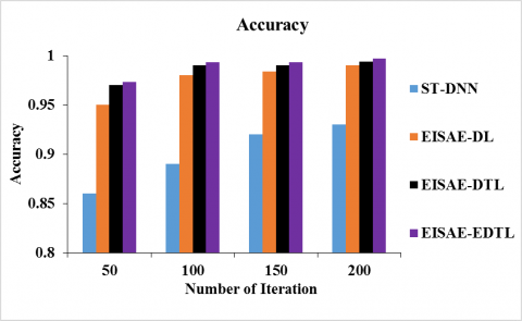
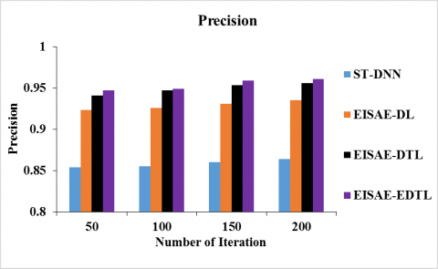
4.1 Accuracy and precision
Accuracy is the estimation of the actual value in the AQ prediction. Also, it is the identification (both valid positive and actual negative values) amongst the number of estimated classes. It is calculated as Eq. (15):
Accuracy $=\frac{T P+T N}{T P+T N+F P+F N}$ (15)
Precision defines the closeness of the measurement and the relevance among the values identified in the AQ prediction. It is calculated as Eq. (16):
Precision $=\frac{T P}{T P+F P}$ (16)
(a)
(b)
Figure 5. Evaluation of (a) accuracy, and (b) precision of EISAE-EDTL with existing works
Figure 5(a) & 5(b) depicts the accuracy & precision of ST-DNN, EISAE-DL, EISAE-DTL and EISAE-EDTL for various iterations. The accuracy (precision) is represented by the Y-axis, while the number of iterations is represented by the X-axis. When the range of iterations is 100, the accuracy (precision) of EISAE-EDTL for AQ prediction is 11.57% (11%), 1.33% (2.5%), and 0.303% (0.21%) higher than ST-DNN, EISAE-DL, and EISAE-DTL. This analysis demonstrates that the EISAE-EDTL exceeds other AQ detection methods in terms of accuracy and precision.
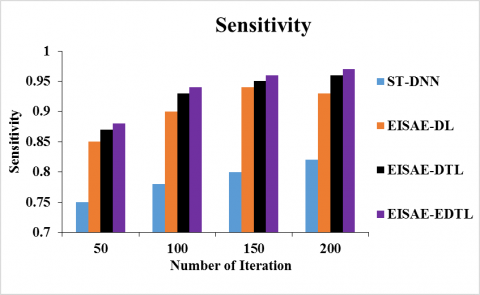
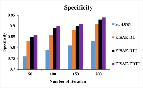
4.2 Sensitivity and specificity
Sensitivity is the fraction of positive values that are adequately identified. It is calculated as Eq. (17):
Sensitivity $=\frac{T P}{T P+F N}$ (17)
Specificity is calculated as the number of correct negative predictions divided by the total number of negatives. It measures the proportion of locations not impacted by air pollution, which is correctly predicted. It is calculated as Eq. (18):
Specificity $=\frac{T N}{T N+F P}$ (18)
Figure 6 (a) and (b) depicts the sensitivity and specificity of ST-DNN, EISAE-DL, EISAE-DTL, and EISAE-EDTL for various iterations. When the number of iteration is set to 100, the sensitivity (specificity) of EISAE-EDTL for AQ estimation is 20.51% (13.92%), and 4.44% (4.65%) and 1.08% (1.12) higher than ST-DNN, EISAE-DL, and EISAE-DTL. This evaluation demonstrates that the suggested EISAE-EDTL has higher sensitivity and specificity than traditional AQ prediction systems.
(a)
(b)
Figure 6. Evaluation of (a) sensitivity, and (b) specificity of EISAE-EDTL with existing works
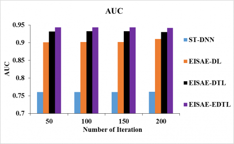
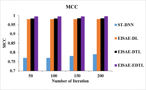
4.3 AUC and MCC
AUC is the prediction indicator and is independent among the classes with distributed instances. It is computed by Eq. (19):
$A U C=\frac{\text { Sensitivity }+\text { Specificity }}{2}$ (19)
MCC is the correlation coefficient between the predicted and actual values. It is calculated as Eq. (20):
$M C C=\frac{T P \times T N-F P \times F N}{\sqrt{(T P+F P)(T P+F N)(T N+F P)(T N+F N)}}$ (20)
Figure 7 (a) and (b) depicts the AUC (MCC) of ST-DNN, EISAE-DL, EISAE-DTL, and EISAE-EDTL for various iterations. When the number of iterations is 100, the AUC (MCC) of EISAE-EDTL for AQ prediction is 24.12% (29.17%) 4.59% (1.52%), and 1.20% (1.138%) higher than ST-DNN, EISAE-DL, and EISAE-DTL. This investigation shows that the EISAE-EDTL has a higher AUC and MCC than classical AQ prediction systems.
Also, the proposed EISAE-EDTL is compared with the related works recently proposed TL-BLSTM [18], and MMSL[20] to show the effectiveness.
(a)
(b)
Figure 7. Evaluation of (a) AUC, and (b) MCC of EISAE-EDTL with existing works
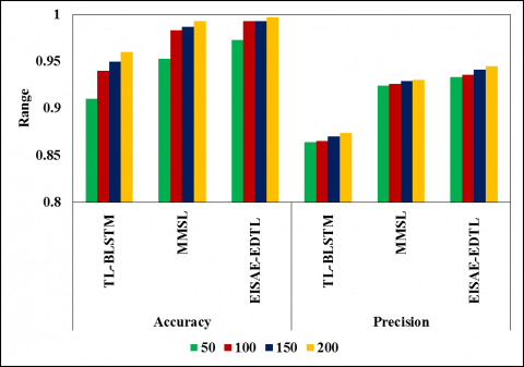
Figure 8. Evaluation of accuracy and precision of EISAE-EDTL with related work
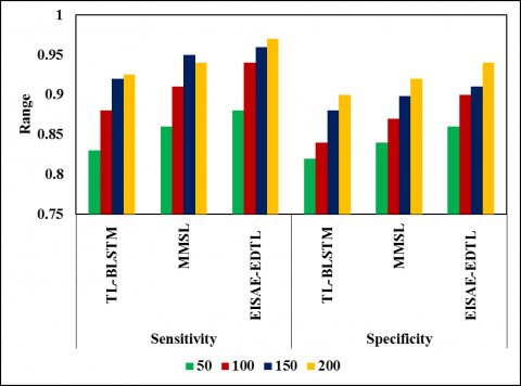
Figure 9. Evaluation of sensitivity and specificity of EISAE-EDTL with related works
Figure 10. Evaluation of AUC and MCC of EISAE-EDTL with related works
Figure 8 depicts the accuracy (precision) of TL-BLSTM, MMSL, and EISAE-EDTL for various iterations. When the range of iterations is 100, the accuracy (precision) of EISAE-EDTL for AQ prediction is 13.45% (12.83%), and 4.12% (3.17%) higher than TL-BLSTM, and MMSL. This analysis shows that the EISAE-EDTL outperforms conventional AQ forecast systems in terms of accuracy and precision.
Figure 9 depicts the sensitivity (specificity) of TL-BLSTM, MMSL, and EISAE-EDTL for various iterations. This analysis demonstrates that the EISAE-EDTL has higher sensitivity and specificity than the classical AQ prediction models.
Figure 10 depicts the AUC (MCC) of TL-BLSTM, MMSL, and EISAE-EDTL for various iterations. When the number of iterations is 100, the AUC (MCC) of EISAE-DTL for AQ prediction is 22.24% (30.78%), and 3.41% (6.26%) higher than TL-BLSTM, and MMSL. According to this analysis, the EISAE-EDTL has a greater AUC and MCC than classical AQ prediction systems.
In this paper, EISAE-DTL and EISAE-EDTL are proposed to handle long-time delay-based locations for better AQ prediction. PM2.5 and PM10 datasets were used to test the proposed models. The significance of pertinent position selection was reaffirmed with the addition of all locations increasing model noise and resulting in poor predicting accuracy. The suggested method surpassed all baselines and comparator models studied. According to the suggested EISAE-EDTL, including an LSTM approach that improved first-hour forecasts with the CNN element being more successful for prolonged detections since CNN might recover the spatial latency factor from neighboring subjective qualities by employing spatial data. In terms of accuracy, precision, specificity, sensitivity, AUC, and MCC, the experimental results suggest that the suggested EISAE-EDTL surpasses current AQ prediction methods.
[1] Pun, V.C., Kazemiparkouhi, F., Manjourides, J., Suh, H. H. (2017). Long-term PM2.5 exposure and respiratory, cancer, and cardiovascular mortality in older US adults. American Journal of Epidemiology, 186(8): 961-969. https://doi.org/10.1093/aje/kwx166
[2] Zhao, Y.M. (2020). Spatial-temporal correlation-based LSTM algorithm and its application in PM2.5 prediction. Revue d'Intelligence Artificielle, 34(1):29-38. https://doi.org/10.18280/ria.340104
[3] Senthivel, S., Chidambaranathan, M. (2022). Machine learning approaches used for air quality forecast: A review. Revue d'Intelligence Artificielle, 36(1): 73-78. https://doi.org/10.18280/ria.360108
[4] Kumar, K., Pande, B.P. (2022). Air pollution prediction with machine learning: a case study of Indian cities. International Journal of Environmental Science and Technology, 1-16. https://doi.org/10.1007/s13762-022-04241-5
[5] Zhang, Y., Wang, Y., Gao, M., Ma, Q., Zhao, J., Zhang, R., Huang, L. (2019). A predictive data feature exploration-based air quality prediction approach. IEEE Access, 7: 30732-30743. https://doi.org/10.1109/ACCESS.2019.2897754
[6] Schürholz, D., Kubler, S., Zaslavsky, A. (2020). Artificial intelligence-enabled context-aware air quality prediction for smart cities. Journal of Cleaner Production, 271: 121941. https://doi.org/10.1016/j.jclepro.2020.121941
[7] Maleki, H., Sorooshian, A., Goudarzi, G., Baboli, Z., Tahmasebi Birgani, Y., Rahmati, M. (2019). Air pollution prediction by using an artificial neural network model. Clean Technologies and Environmental Policy, 21(6): 1341-1352. https://doi.org/10.1007/s10098-019-01709-w
[8] Yang, W., Deng, M., Xu, F., Wang, H. (2018). Prediction of hourly PM2. 5 using a space-time support vector regression model. Atmospheric Environment, 181: 12-19. https://doi.org/10.1016/j.atmosenv.2018.03.015
[9] Syafei, A.D., Fujiwara, A., Zhang, J. (2015). Prediction model of air pollutant levels using linear model with component analysis. International Journal of Environmental Science and Development, 6(7): 519-525. https://doi.org/10.7763/IJESD.2015.V6.648
[10] Soh, P.W., Chen, K.H., Huang, J.W., Chu, H.J. (2017). Spatial-Temporal pattern analysis and prediction of air quality in Taiwan. In 10th IEEE International Conference on Ubi-media Computing and Workshops, Pattaya, Thailand, Pattaya, Thailand, pp. 1-6. https://doi.org/10.1109/UMEDIA.2017.8074094
[11] Wang, J., Song, G. (2018). A deep spatial-temporal ensemble model for air quality prediction. Neurocomputing, 314: 198-206. https://doi.org/10.1016/j.neucom.2018.06.049
[12] ShreeNandhini, P., Amudha, P., Sivakumari, S. (2022). Comparative analysis of air quality prediction using artificial intelligence techniques. ECS Transactions, 107(1): 6059. https://doi.org/10.1149/10701.6059ecst
[13] Qin, S., Liu, F., Wang, C., Song, Y., Qu, J. (2015). Spatial-temporal analysis and projection of extreme particulate matter (PM10 and PM2.5) levels using association rules: a case study of the Jing-Jin-Ji region, China. Atmospheric Environment, 120: 339-350. https://doi.org/10.1016/j.atmosenv.2015.09.006
[14] Jiang, F., He, J., Tian, T. (2019). A clustering-based ensemble approach with improved pigeon-inspired optimization and extreme learning machine for air quality prediction. Applied Soft Computing, 85: 1-30. https://doi.org/10.1016/j.asoc.2019.105827
[15] Lin, Y.C., Lee, S.J., Ouyang, C.S., Wu, C.H. (2020). Air quality prediction by neuro-fuzzy modeling approach. Applied Soft Computing, 86: 1-13. https://doi.org/10.1016/j.asoc.2019.105898
[16] Soh, P.W., Chang, J.W., Huang, J.W. (2018). Adaptive deep learning-based air quality prediction model using the most relevant spatial-temporal relations. IEEE Access, 6: 38186-38199. https://doi.org/10.1109/ACCESS.2018.2849820
[17] Mao, W., Wang, W., Jiao, L., Zhao, S., Liu, A. (2021). Modeling air quality prediction using a deep learning approach: method optimization and evaluation. Sustainable Cities and Society, 65: 1-25. https://doi.org/10.1016/j.scs.2020.102567
[18] Ma, J., Cheng, J.C., Lin, C., Tan, Y., Zhang, J. (2019). Improving air quality prediction accuracy at larger temporal resolutions using deep learning and transfer learning techniques. Atmospheric Environment, 214: 1-10. https://doi.org/10.1016/j.atmosenv.2019.116885
[19] Zhang, L., Liu, P., Zhao, L., Wang, G., Zhang, W., Liu, J. (2020). Air quality predictions with a semi-supervised bidirectional LSTM neural network. Atmospheric Pollution Research, 12(1): 328-339. https://doi.org/10.1016/j.apr.2020.09.003
[20] Seng, D., Zhang, Q., Zhang, X., Chen, G., Chen, X. (2021). Spatiotemporal prediction of air quality based on LSTM neural network. Alexandria Engineering Journal, 60(2): 2021-2032. https://doi.org/10.1016/j.aej.2020.12.009
[21] Cheng, C., Zhou, B., Ma, G., Wu, D., Yuan, Y. (2020). Wasserstein distance based deep adversarial transfer learning for intelligent fault diagnosis with unlabeled or insufficient labeled data. Neurocomputing, 409: 35-45. https://doi.org/10.1016/j.neucom.2020.05.040
[22] Ferrero, L., Bolzacchini, E., Petraccone, S., Perrone, M. G., Sangiorgi, G., Porto, C.L., Ferrini, B. (2007). Vertical profiles of particulate matter over Milan during winter 2005/2006. Fresenius Environmental Bulletin, 16(6): 697-700.
[23] Ma, J., Li, Z., Cheng, J.C., Ding, Y., Lin, C., Xu, Z. (2020). Air quality prediction at new stations using spatially transferred bi-directional long short-term memory network. Science of the Total Environment, 705: 1-10. https://doi.org/10.1016/j.scitotenv.2019.135771
[24] Kurt, A., Oktay, A.B. (2010). Forecasting air pollutant indicator levels with geographic models 3 days in advance using neural networks. Expert Systems with Applications, 37(12): 7986-7992. https://doi.org/10.1016/j.eswa.2010.05.093