Shweta M. Madiwal* | Vishwanath Burkpalli
© 2022 IIETA. This article is published by IIETA and is licensed under the CC BY 4.0 license (http://creativecommons.org/licenses/by/4.0/).
OPEN ACCESS
Skin cancer is becoming major problems due to its tremendous growth. Skin cancer is a malignant skin lesion, which may cause damage to human. Hence, prior detection and precise medical diagnosis of the skin lesion is essential. In medical practice, detection of malignant lesions needs pathological examination and biopsy, which is expensive. The existing techniques need a brief physical inspection, which is imprecise and time-consuming. This paper presents a computer-assisted skin cancer detection strategy for detecting the skin lesion in skin images using deep stacked auto encoder. Sine Cosine-based Harris Hawks Optimizer (SCHHO) trains deep stacked auto encoders. The proposed SCHHO algorithm is designed by combining Sine Cosine Algorithm (SCA) and Harris Hawks Optimizer (HHO). The identification of skin lesion is performed on each segment, which is obtained by sparse-Fuzzy-c-means (FCM) algorithm. Statistical features, texture features and entropy are employed for selecting the most significant feature. Mean, standard deviation, variance, kurtosis, entropy, and Linear Discriminant Analysis (LDP) featured are extracted. SCHHO-Deep stacked auto-encoder outperformed other approaches with 91.66% accuracy, 91.60% sensitivity, and 91.72% specificity.
skin cancer detection, skin cancer lesions, deep stacked auto-encoder, LDP, entropy
The cancer is considered as foremost contributor for causing a sudden upsurge in mortality rate all over the world. There exist different kinds of cancer which are determined earlier for the prior diagnosis. However, skin cancer is a major disease that tends to be a fast-growing cancer these days. As per machine research, the patients undergoing skin cancer detection are continuously growing compared to other types of cancer [1]. For both dermatologists and oncologists, the notion of early identification of skin melanoma cancer is crucial since it increases the likelihood of achieving full oncological remission. The histology of melanoma is complicated domain as late diagnosis may increase the mortality rates. The detection of skin lesion needs high experience and competence and thus the medical diagnosis is a challenging task [2]. As compared to other kinds of skin cancer, the melanoma is not frequent but it is likely to spread and grow. Skin tumor like other tissue tumors can be benign or malignant. The status and nature of skin cancer is different and thus it can be hard, soft, moving, losing or deep with respect to size or shape [3]. Melanoma cancer is considered as an advanced phase that might overrun internal organs like lungs through blood vessels, by building the treatment even difficult. Meanwhile, Early detection is key to treating melanoma, thus dermatologists recommend routine skin checks to increase the likelihood of an accurate diagnosis. Dermatologists use digital imaging to identify and treat skin cancer [4].
The most common cancer among those with fair skin is skin cancer, and as non-melanoma and melanoma cases increase in frequency, the associated medical expenses rise. Earlier melanoma diagnosis tends to improve patient outcomes and identification of skin cancer can be enhanced by screening patients using intensive skin symptoms considering examination of overall body skin [5]. As skin cancer provides epidermis which is the uppermost skin layer as it is relatively visible. This technique illustrates that the CAD model may utilise skin cancer photos without considering other important information. Skin cancer is a leading cause of mortality. Melanoma affects the skin’s melanocytes. This cancer contains cells which may cause the skin go black color. The Melanoma may lead to metastasis and has the capability to spread. Melanoma can be determined anywhere on the human which is on the human legs.
Discovery of skin cancer in the earlier stage may lead to effectual treatment and can be attained by the automatic determination of cancer types considering deep learning methods. The results show that deep convolutional neural networks (DCNNs) may be utilized to accurately and automatically identify skin cancer [6]. In recent days, the quicker extension in deep learning made prodigious accomplishments in several tasks of computer vision. Deep learning uses many processing layers to extract features and change data. Convolutional neural networks (CNN) is the major deep learning techniques that attained prodigious empirical successes in the computer aided diagnosis [7]. The analysis is performed in particular domain to precisely identify the skin cancer. Tenderness of the skin and the categorization of skin either as benign or melanoma is performed using different models like genetic algorithms, support vector machines (SVMs), artificial neural networks (ANNs), and CNNs. All given methods tend to be cost-effective and highly effective and less painful than existing medical models. However, in several computer vision problems, it is indisputable that both deep learning and CNNs are the mostly used technique [8]. The majority of the classification techniques are applied on the computer-based melanoma recognition models which involve SVM [9], Bayes networks, ANN [10], discriminate analysis [11], k-nearest neighbourhood, decision trees [12], and logistic regression. On the other hand, some advanced models of these classifiers are modelled in the existing works which includes random forest [13], hidden naive Bayes, and logistic model tree [14].
The difference between the depth automatic encoder and stacked automatic encoder is the way the two networks are trained. Depth automatic encoders are trained in the same way as a single-layer neural network, while stacked automatic encoders are trained with a greedy, layer-wise approach so the training time required to train the depth automatic encoders is less compared to that of stacked automatic encoders.
Proposed SCHHO-based Deep stacked auto-encoder is used in current research to present a skin cancer detection approach. Research’s contribution is the use of statistical and textural data to identify skin lesions. Here, the segments from which the malignant patches are diagnosed are obtained using the sparse FCM. Mean, standard deviation, variance, kurtosis, entropy, and LDP are extracted to detect lesions. A deep stacked auto-encoder finds skin lesions using these characteristics. Deep stacked auto-encoder is trained using SCHHO to learn model parameters. The suggested algorithm, SCHHO, was created by inheriting high global convergence property from HHO procedure. Therefore, deep stacked auto-encoder based on SCHHO offers effective accuracy while enabling skin cancer detection. The SCA and HHO algorithms are combined in the suggested SCHHO algorithm. Main contribution of paper is:
Proposed SCHHO-based Deep stacked auto-encoder for detection of skin cancer: Deep stacked auto-training encoder’s approach is modified with SCHHO algorithm that is newly created by combination of SCA and HHO algorithms, for best tuning of weights and biases. This classifier is known as the SCHHO-based Deep stacked auto-encoder. In order to identify lesions in skin images, recommended SCHHO-based Deep stacking auto-encoder has been updated.
The remaining portions in this paper are: The conventional skin cancer detection methods used in the literature and the difficulties encountered are outlined in Section 2 and are used as inspiration for the suggested method’s development. In Section 3, the Deep stacked auto-encoder approach for skin cancer identification is described. In Section 4, the outcomes of the suggested approach compared to other methods are shown, and Section 5 concludes.
Melanoma is a severe kind of skin cancer that can have life-threatening effects on people. In order to increase the chance of survival, skin cancer should be accurately and promptly diagnosed. Since melanoma and non-melanoma have similar appearances, it might be difficult to diagnose various lesion situations with accuracy. As a result, a crucial step in enabling good lesion classification is creating an effective lesion representation utilising an optimization technique. Eight currently used methods for detecting skin cancer are examined here, and each approach's shortcomings served as inspiration for the development of a new skin cancer identification method.
2.1 Literature survey
An overview of eight existing methods for skin cancer identification is devised here. Burlina et al. [15] utilized deep convolutional neural network with a cross-sectional dataset containing images for training the model to perform classification. The capability of machine was computed to categorize the type of skin using the set of input images. The method provided precise diagnosis, but failed to involve other skin pathologies for distinguishing erythema, like cellulitis. Pandey et al. [16] devised multi-scale retinex with color restoration (MSR-CR) method for addressing the issues of skin cancer detection considering image enhancement methods for detecting the skin cancer. The method provided improved results with poor quality images, but faced several environmental complexities. Tan [17] devised intelligent decision support system for determining skin cancer. Here, two enhanced PSO models were devised for optimizing the features. The first model used remote leaders and adaptive acceleration coefficients for overwhelming the issues of stagnation. The second model employed random acceleration coefficients for enhancing the intensification and diversification. The approach, however, did not work with other types of medical picture data. A DCNNs based on Gabor wavelets was developed by Serte and Demirel for the purpose of identifying malignant melanoma from the photos. The technique was developed based on directional subbanding of the input pictures into seven different directions. Decision fusion with sum-rule was employed for classifying the skin lesion. The method enhanced overall performance, but was unable to deal with low contrast images. Zhao et al. [7] devised a dataset of Hospital Central South University for skin cancer detection. The images are divided into risk grades with different degree of malignancy. The method was capable to automatically grade the image containing skin tumour. The method was useful to patients undergoing initial screening before diagnosis, but the method failed to use images of different ages and ethnicities. Dorj et al. [18] utilized an intelligent and rapid classification system for skin cancer detection utilizing DCNN, and SVM. Here, pre-trained AlexNet CNN model was employed for extracting the significant features. Method enhanced the overall performance of system, but failed to utilize asymmetry, border, color, and diameter (ABCD) rule for detecting skin cancer. Saba [19] developed an approach for identifying the skin lesion and recognizing the cancerous regions using DCNN. The three main phases of the approach were lesion boundary extraction, contrast enhancement, and the extraction of depth characteristics. Additionally, the most important characteristics were chosen using an entropy-controlled feature selection approach. The method was effective, but failed to employ physics selection theorems to select optimum features. Kawahara et al. [5] employed multi-task DCNN using multi-modal data for classifying the melanoma to diagnose the skin cancer. The neural network was trained with different multi-task loss functions in which each loss consider multiple combinations of input modalities for skin cancer detection However, this model failed to detect the labels. Patil et al. [20-23] proposed techniques to classify melanoma, type of melanoma and stage of melanoma.
2.2 Challenges
The challenges encountered in automatic detection of skin cancer are as following:
In comparison to using only the naked eye, dermatoscopy increased the analytical accuracy of pigmented skin lesions. However, accurate diagnosis is a difficult process for amateurs [18].
As per diagnostic standards, the skin tumors can be categorized into different classes like high degree malignancy, benign or low degree malignancy. However, the determination of high degree malignant skin tumors may lead to serious issues if not detected in correct time and may require more time [8].
The automatic detection of melanoma is a challenging issue due to changing shapes, and texture of lesions. Other artifacts, like illumination color calibration, illumination, affect the segmentation process and minimize the accuracy of feature extraction [5].
To find skin cancer, an intelligent decision-support system is created. The approach is effective in classifying the lesion, however it is difficult to provide a precise diagnosis of various lesions [16].
The occurrence of skin tumors has progressively augmented. Even though, most of them are benign and does not influence the survival and some of the malignant skin tumors confronts delay in diagnosis. An ideal assessment by the skilled dermatologist would precisely determine the malignant skin tumors in the earlier stage, but it is not practical for each single patient to undergo rigorous screening by dermatologists.
SCHHO-based deep stack auto-encoder is presented for automated skin cancer diagnosis, extracting statistical and textural information for classification. The input skin images are first pre-processed to prepare them for subsequent processing. Images that have been previously processed are then subjected to a segmentation module, where they are segmented using Sparse FCM [24]. After getting the segments, each segment is taken into account while performing the feature extraction. Each segment's statistical characteristics are extracted.
Figure 1. Block diagram of proposed SCHHO-based Deep Stacked auto-encoder method
Feature vectors include each segment's retrieved features. Using the feature vector, a deep stacked auto encoder [24] trained with SCHHO detects skin cancer. Standard HHO and SCA are combined to create the suggested SCHHO, which inherits the benefits of both optimizations for efficient classifier training. The proposed SCHHO-based deep stacked auto encoder is used to depict framework for identification of skin cancer in Figure 1.
Simplify the diagram in Figure 1. Draw only four blocks and label them appropriately indicating functionality of each block: preprocessing, segmentation, extraction of feature and categorization. Assume a skin cancer dataset G with f number of skin images, it is given as:
$G=\left\{I_1, I_2, \ldots, I_g, \ldots, I_f\right\}$ (1)
where, Ig is gth input image, and f is the overall amount of images.
3.1 Pre-processing utilizing skin cancer images
To remove noise and artefacts from image, pre-processing is used. The pre-processing may also be used as an image improvement module to boost contrast of the picture for the aim of identifying skin cancer. The pre-processed pictures are concurrently entered into segmentation to determine the relevant characteristics suitable for the diagnosis of skin cancer.
3.2 Segmentation of preprocessed image
Preprocessed image is input to segmentation unit while taking into account the Sparse FCM method [24]. Sparse FCM is a variant of normal FCM, and it offers high dimensional data clustering as a benefit. The pre-processed image has many segments, each of which denotes a distinct region. The sparse FCM is used in the skin cancer detection approach for image segmentation.
Consider image pixels as V, data matrix as $D=\left(V_{k l}\right) \in {\Re} ^{p \times q}$, p and q are image size. The programme forms clusters to make skin cancer diagnosis easier. Sparse FCM outputs segments. Steps of sparse FCM is described below.
1. Initially, feature weights are initialized and are represented as $\omega=\omega_1^e=\omega_2^e=\ldots=\omega_q^e=\frac{1}{\sqrt{q}}$. Pixel location is determined by features considering q=2.
2. At first, attribute weights $\omega$ and cluster centres $S \varepsilon(\Re)$ is reduced when:
$P_{k t}=\left\{\begin{array}{l}\frac{1}{N_t} ; \text { if } B_{k t}=0 \text { and } N_t=\operatorname{card}\left\{l: B_{k t}=0\right\} \\ 0 ; \text { if } B_{k t} \neq 0 \text { but } B_{k j}=0 \text { forsome } j, j \neq t \\ \frac{1}{\sum_{j=1}^n\left(\frac{B_{k t}}{B_{j t}}\right)\left(\frac{1}{\beta-1}\right)} ; \text { Otherwise }\end{array}\right.$ (2)
where, card(A) indicates cardinality of set A. Distance adapted in sparse-FCM is modelled as:
$B_{k t}=\sum_{t=1}^n \omega_l\left(V_{k l}-V_{t l}\right)^2$ (3)
3. Assume ω and $\Re$ be fixed and ε(S) is reduced if:
$S_{t l}=\left\{\begin{array}{l}0 ; i f \omega_l=0 \\ \frac{\sum_{i=1}^n P_{k t}^\beta \cdot V_{k l}}{\sum_{k=1}^n P_{k t}^\beta} ; \text { if } \omega_l \neq 0\end{array}\right.$ (4)
where, t=1, ..., n and l=1, ..., q, β indicate weight component, and is liable to control membership degree using fuzzy clusters. Role of lth feature in objective function is represented as, ωl and dissimilarity measure is represented as, $\Re$.
4. Class value is found using fixed clusters $\left\{s_1, s_2, \ldots, s_i, \ldots, s_n\right\}$ and the membership $P$. Class $G_l$ is evaluated on basis of following objective, $\max _\omega \sum_{l=1}^q \omega_l . G_l$ such that $\|\omega\|_2^2 \leq 1,\|\omega\|_f^f \leq \ell$ and obtain $\omega^*$.
where, $\ell$ indicate tuning parameter and $(0 \leq f \leq 1) ;\|\omega\|_f^f=$ $\sum_{l=1}^q\left|\omega_l\right|^f$
5. Iterate till halting requirement met. Stopping criterion:
$\frac{\sum_{l=1}^q\left|\omega_l^*-\omega_l^e\right|}{\sum_{l=1}^q\left|\omega_l^e\right|}<10^{-4}$ (5)
Sparse FCM outputs image segments as:
$S=\left\{s_1, s_2, \ldots, s_i, \ldots, s_n\right\}$ (6)
where, r indicates count of segments generated from preprocessed image.
3.3 Using statistical and texture characteristics, generation of a feature vector
Following the acquisition of segments, features are retrieved from the pre-processed image taking into account each segment. Statistical aspects like mean, variance, standard deviation, kurtosis, and entropy as well as texture features like LDP are among the features retrieved from the segments and are described below.
Mean: The average is determined by counting all of the pixels in image that are expressed as:
$\mu=\frac{1}{\left|d\left(S_n\right)\right|} \times \sum_{n=1}^{\left|d\left(S_n\right)\right|} d\left(S_n\right)$ (7)
where, n is the total number of segments, values of each segment's pixels, and |d(Sn)| is total number of pixels included in the segment
Variance: Based on the mean value, which is written as, the variance feature is computed as:
$\sigma=\frac{\sum_{n=1}^{\left|d\left(S_n\right)\right|}\left|S_n-\mu\right|}{d\left(S_n\right)}$ (8)
Standard deviation: Square root of variance is used to get standard deviation, which is represented by ρ.
Kurtosis: It represents evenness that defines sharpness of peak. It defines shape of an object depending on its numerical value. Probability distribution's relative peakedness is shown by the kurtosis.
Entropy: Entropy is a common metric for quantifying uncertainty in data and is applied to increase mutual information in various procedures. Appropriateness preference for a specific operation was motivated by the abundance of entropy variations. In order to pinpoint the difference between adjacent pixels or a pixel group, entropy of an image is used. Entropy is further defined as comparable intensities levels to which individual pixels can adapt. An image's entropy can be utilised for quantitative analysis, evaluation of the image's details, and better comparison of image details. As a result, the resulting probability's entropy is calculated and is represented as:
$\varepsilon=-Q \log (Q)$ (9)
where, Q is pixel probability distribution in an image.
LDP: Local Directional Pattern (LDP) [25] is a directional component that incorporates a local pattern descriptor by altering Kirsch compass kernels. In comparison to the LBP operators now in place, the LDP is less noise sensitive.
$L=L D P_c\left(a_n, b_n\right)=\sum_{x=0}^7 v\left(b_x-b_c\right) \cdot 2^x$ (10)
where, c signifies pixel location, (an, bn) denotes directed bit responses, x neighborhood pixel number, bx denotes Kirsch masks, and bc denote cth directional response.
$v(a)=\left\{\begin{array}{l}1 ; \text { if } a \geq 0 \\ 0 ; \text { otherwise }\end{array}\right\}$ (11)
3.3.1 Formation of feature vector
Collection of statistical and texture features is shown in Eq. (12). Consequently, each segment’s characteristics are presented as follows:
$J=\{\mu, \sigma, \rho, \kappa, \varepsilon, L\}$ (12)
where, J denotes feature vector which is extracted utilizing each segment, $\mu, \sigma, \rho, \kappa$ and $\varepsilon$ denote mean, variance, kurtosis, standard deviation, and entropy are the statistical features, whereas texture features include LDP that is represented by L. Deep stacked auto encoder receives feature vector, which it uses to classify input images based on features and determine class label. Classifier determines class label and divides input image's malignant and non-cancerous areas into categories.
3.4 The proposed SCHHO-based deep stacked auto encoder
This section describes how to identify skin cancer using the suggested SCHHO approach and how to advance the detection using a feature vector. Deep stacked auto encoder [26] is used to present extracted features for classification, and the suggested training algorithm SCHHO—a combination of the SCA and the HHO —is utilized to train classifier. Proposed SCHHO’s objective is to use the extracted features to detect malignant areas in input image. The inclusion of SCA in HHO is the planned SCHHO. Here, the sine and cosine functions are taken into account when designing the SCA algorithm. The algorithm is adept at balancing exploitation and exploration states to identify search spaces most promising regions and assists in obtaining the global optimum. The strategy benefits from the avoidance of local optima and high exploration, therefore resolving practical issues. HHO, on the other hand, draws inspiration from Harris hawks submissive conduct and chasing manner. The approach is efficient in handling various optimization problems that can result in efficient solutions. HHO can handle misleading optima, local optimum solutions, and multi-modality. To enhance the algorithm’s overall performance, SCA and HHO are integrated. The following describes the proposed SCHHO’s algorithmic phases as well as the deep stacked auto encoder's architecture.
3.4.1 Architecture of deep stacked auto encoder
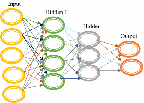
Auto Encoder in Deep Neural Networks (DNN) is crucial. The relevant input characteristics are used by the auto encoder. The single layer auto encoder does not have directed loops in its output visible units, which are also hidden units at the encoder's input. Figure 2 shows the deep stack auto encoder's structural arrangement. Encoding input vector into an advanced phase concealed version, shown as K, advances auto encoder.
Figure 2. Architecture of deep stack auto-encoder
Deep Neural Networks use Auto Encoder (DNN). Auto encoder inputs are used. Single-layer auto encoder input visible units are concealed, and output visible units don't contain directed loops. Figure 2 shows the encoder's structural arrangement. The auto encoder advances by encoding input vector as K. In encoder, deterministic mapping Tθ turns input vector into hidden vector X.
$\vartheta=\operatorname{fun}\left(\omega_1 U+R_1 U\right)$ (13)
where, R1 is to the bias vector, and U is reconstruction, and ω1 indicates the weight matrix. The equation will be written as after decoding the concealed version back to reconstruction:
$\widehat{U}=\operatorname{fun}\left(\omega_2 Y+R_2 Y\right)$ (14)
where, ω2 represent weight matrix, R2 denote bias vectors, and Y hidden units.
Back propagation encounters difficulties with local minima and sluggish convergence. The frequent weight changes are what cause the local minima. Additionally, the Back propagation algorithm does not require input vector normalization. System’s performance can be improved by normalizing, however this technique does not allow for the determination of the error function's global minimum. Auto Encoder is trained utilizing SCHHO instead of back propagation to reduce cost function and squared reconstruction error.
$\operatorname{Jac}(\omega, R)=\frac{1}{2 z} \sum_{x=1}^z\left\|\widehat{U}_x^z-U_x^X\right\|^2$ (15)
where, ω weight set, R bias vectors, z total layers where 1≤x≤z, $U_x^z$ displays the input xth and $U_x^X$ output reconstructions on $x^{t h}$ layer.
To prevent overfitting, a weight regularisation term and scarcity restrictions are used to create a cost function.
$\operatorname{Jac}(\theta)=\frac{1}{z} \sum_{x=1}^z\left\|U_x^z-U_x^X\right\|^2+\alpha\left(\left\|\omega_1\right\|^2+\right.\left.\left\|\omega_2\right\|^2\right)+\beta \sum_{y=1}^Y V\left(U \| U_y\right)$ (16)
where, $U_x^z$ represents input reconstruction on xthlayer and $U_x^X$ demonstrates output reconstruction on xth layer, α is weight for regulation condition, and β is weight for sparse condition, and $\mid \omega_1\left\|^2+\right\| \omega_2 \|^2$ denotes parametric conditions, U is the sparse parameter, and Uy denotes average activation of hidden unit y, and V(U||Yy) denotes Kullback Leibler divergence, and Y is number of hidden units like 1≤y≤Y. Average hidden unit is formulated as:
$\widehat{U}_y=\frac{1}{z} \sum_{x=1}^z l_{2, x}^y$ (17)
where, $l_{2, x}^y$ denote hidden layer activation function of yth entry, and z denote total layers where 1≤x≤z. Kullback Leibler divergence is formulated as:
$V\left(U \| U_y\right)=U \log \frac{U}{U_y}+(1-U) \log \frac{1-U}{1-U_y}$ (18)
where, U denotes sparse parameter, and Uy denotes average activation of hidden unit y. The auto-encoder is made up of a number of layers of sparse auto encoder, the outputs of which are coupled to the inputs of succeeding layers, where Y1, Y2, and Y3 depicts hidden layers. Concatenation of auto-encoders that inputs of next layers are connected to outputs of auto-encoders stacked on layer. Auto-encoders are finally layered in a hierarchical fashion. Activation output of zth layer is given as:
$l_{q x}^X=w q\left(l_{q-1}^X \omega_{q-1}+s_{q-1}^X\right)$ (19)
where, l1,x=ux. By describing $p_{\omega, O}\left(u_x^X\right)=l_{o, x}$, cost function is:
$\operatorname{jac}(\omega, O)=\frac{1}{2 z} \sum_{x=1}^z\left\|p_{\omega, O}\left(u_x^X\right)-u_x\right\|^2$ (20)
$\begin{aligned} \operatorname{jac}(\theta)=j a c(\omega, O) & +\frac{\alpha}{2} \sum_{q=1}^{i_z-1} \sum_{n=1}^{j_z} \sum_{o=1}^{j_{z+1}}\left(\omega_q^{n, o}\right)^2 +\sum_{q=z}^{i_z-1} \sum_{y=1}^{j_z} \gamma^q V\left(U^q \| \widehat{U}_y^q\right)\end{aligned}$ (21)
where, iq denote total layers in the network, γq and Uq represents hyper parameters in qth layer.
So, there are three processes involved in processing the deep stack auto encoder. The initialization of parameters close to a local minimum for each unique auto-encoder is first stage. Learning hidden layer activations of next auto-encoder hidden layer is second stage. Using suggested SCHHO method, the fine tuning is carried out in the third stage. Each parameter in this model is changed concurrently to improve classification outcome.
3.4.2 Training of deep stacked auto encoder using SCHHO
SCHHO method is utilized to train deep stacked auto encoder classifier for skin cancer detection. This section explains how the SCHHO algorithm was implemented. The SCHHO method is utilized to build the optimal weights, which are then used to fine-tune the deep stacked auto encoder. Skin cancer identification uses a SCHHO-based deep stacked auto encoder to recognize input photos and manage fresh images from dispersed sources. Below are the SCHHO algorithmic steps:
Step 1: Initialize solution and parameters.
$A=\left\{A_1, A_2, \ldots, A_a, \ldots A_v\right\}$ (22)
where, v is total number of solution and Aa is position of $a^{t h}$ solution.
Step 2: The solution with least Mean Square Error (MSE) is best based on fitness function, or minimization problem. Here's how to compute MSE:
$M S E=\frac{1}{f} \sum_{g=1}^f\left[F_g-F_g^*\right]^2$ (23)
where, Fg expected output and $F_g^*$ predicted output, f represents number of data samples, where 1<g≤f.
Step 3. The SCA addresses real-world problems by avoiding local optima by investigating global optimum. SCA method is very efficient and gives higher performance while assessing solutions. It requires fewer parameters for fine tuning and has a simpler algorithmic framework. Solution update per SCA algorithm [9]:
$A^{o+1}=\left\{\begin{array}{l}A_j^o+h_1 \operatorname{Sin}\left(h_2\right) \times\left|h_3 M_j^o-A_j^o\right| ; h_4<0.5 \\ A_j^o+h_1 \operatorname{Cos}\left(h_2\right) \times h_3 M_j^o-A_j^o \mid ; h_4 \geq 0.5\end{array}\right.$ (24)
where, r1 indicate movement direction, r2 determines how far movement should be towards or outwards the destination, r3 provides random weight for destination, and r4 helps to switch between sine and cosine components, $A_j^o$ indicate the current solution, and $M_j^o$ represent the position of destination point in jth dimension and ||indicate absolute value.
The HHO algorithm is used to enhance algorithm performance and handle optimization problems. In accordance with HHO [10], the update equation is written as:
$A^{l+1}=A_{r a b}^l-H\left|\Delta A^t\right|$ (25)
where, $A_{r a b}^l$ represent the position of rabbit, $\Delta A^t$ indicate difference between position of rabbit and current position, and ![]() represent escaping energy of prey. The above equation is also referred as:
represent escaping energy of prey. The above equation is also referred as:
$A^{l+1}=A_{r a b}^l-H\left|A_{r a b}^l-A^l\right|$ (26)
Considering $A_{r a b}^l>A^l$,
$A^{l+1}=A_{r a b}^l-H\left(A_{r a b}^l-A^l\right)$ (27)
$A^{l+1}=A_{r a b}^l-H A_{r a b}^l+H A^l$ (28)
$A^{l+1}=A_{\text {rab }}^l(1-H)+H A^l$ (29)
$A_{r a b}^l=\frac{A^{l+1}-H A^l}{1-H}$ (30)
As $A_{r a b}^l$ represent the target position in HHO, and $M_j^l$ indicate destination location in SCA, both can be equated:
For h4<0.5,
$A^{l+1}=A^l+h_1 \operatorname{Sin}\left(h_2\right) \times\left(h_3\left(\frac{A^{l+1}-H A^l}{(1-H)}\right)-A^l\right)$ (31)
$A^{l+1}=A^l+h_1 \operatorname{Sin}\left(h_2\right) \times\left(\frac{h_3 A^{l+1}}{1-H}-\frac{h_3 H A^l}{1-H}-A^l\right)$ (32)
$A^{l+1}=A^l+h_1 \operatorname{Sin}\left(h_2\right) \frac{h_3 A^{l+1}}{1-H}-h_1 \operatorname{Sin}\left(h_2\right) \frac{h_3 H A^l}{1-H}-h_1 \operatorname{Sin}\left(h_2\right) A^l$ (33)
$A^{l+1}-h_1 \operatorname{Sin}\left(h_2\right) \frac{h_3 A^{l+1}}{1-H}=A^l(1-\left.h_1 \operatorname{Sin}\left(h_2\right)\left(\frac{h_3 H}{1-H}+1\right)\right)$ (34)
$A^{l+1}\left(1-\frac{h_1 \operatorname{Sin}\left(h_2\right) h_3}{1-H}\right)=A^l\left(1-h_1 \operatorname{Sin}\left(h_2\right)\left(\frac{h_3 H}{1-H}+1\right)\right)$ (35)
$A^{l+1}\left(\frac{1-H-h_1 \operatorname{Sin}\left(h_2\right) h_3}{1-H}\right)=A^l\left(1-h_1 \operatorname{Sin}\left(h_2\right)\left(\frac{h_3 H}{1-H}+1\right)\right)$ (36)
$A^{l+1}=\frac{1-H}{1-H-h_1 h_3 \operatorname{Sin}\left(h_2\right)}\left[A^l\left(1-h_1 \operatorname{Sin}\left(h_2\right)\left(\frac{h_3 H}{1-H}+1\right)\right)\right]$ (37)
Likewise for h4≥0.5,
$A^{l+1}=\frac{1-H}{1-H-h_1 h_3 \operatorname{Cos}\left(h_2\right)}\left[A^l\left(1-h_1 \operatorname{Cos}\left(h_2\right)\left(\frac{h_3 H}{1-H}+1\right)\right)\right]$ (38)
Consequently, the final update equation is written as:
$A^{l+1}=\left\{\begin{array}{l}\frac{1-H}{1-H-h_1 h_3 \operatorname{Sin}\left(h_2\right)}\left[A^l\left(1-h_1 \operatorname{Sin}\left(h_2\right)\left(\frac{h_3 H}{1-H}+1\right)\right)^{\prime}\right] ; h_4<0.5 \\ \frac{1-H}{1-H-h_1 h_3 \operatorname{Cos}\left(h_2\right)}\left[A^l\left(1-h_1 \operatorname{Cos}\left(h_2\right)\left(\frac{h_3 H}{1-H}+1\right)\right)^i\right] ; h_4 \geq 0.5\end{array}\right.$ (39)
In Eq. (39), exploration and exploitation are balanced by updating cosine and sine ranges as the iteration counter grows. SCA trades off exploration and exploitation to identify the best answers.
Step 4: Recalculating error utilizing equation’s answer (23). The deep stacked auto encoder is trained to find skin cancer using method that produces the least amount of error.
Step 5: The suggested SCHHO method recomputes each solution’s error and evaluates them such that the solution with the least error is utilized to train the deep stacked auto encoder.
Step 6: Iteratively determining optimum weights till the maximum number of iterations. Table 1 shows SCHHO's pseudocode.
Table 1. Pseudo code of proposed SCHHO method
|
Begin |
|
Initialize set of solutions |
|
Do |
|
Evaluate each solution with MSE using Eq. (23) |
|
Update the best solution obtained till execution |
|
Update h1, h2, h3 and h4 |
|
Update the solution using Eq. (39) |
|
While (l<lmax) |
|
Return optimum solution |
4.1 Experimental setup
Proposed system is executed in MATLAB utilizing Windows 10 OS, 2GB RAM, and Intel i3 core processor.
4.2 Dataset description
HAM10000 database [27] consist of pigmented lesions using different populations. The dataset contains 10015 dermatoscopic images, which are employed as the training set for machine learning and available in ISIC 2019 archive. The dataset contains a collection of significant diagnostic using pigmented lesions. We have use 80% dataset for training and 20% dataset for testing.
4.3 Experimental result
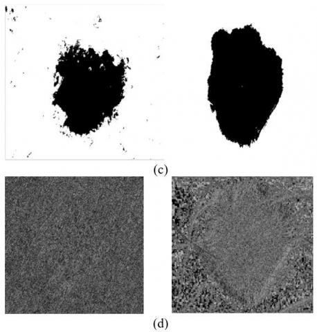
Figure 3 shows experimental results of proposed SCHHO-Deep stacked auto-encoder using set of input skin images. Figure 3a) shows input images acquired from skin cancer dataset. Figure 3b) shows segmented image, 3c) portrays the binary image and 3d) displays the LDP applied image for skin cancer detection. In segmented image, the bluish part represents the region affected by the cancer, whereas in binary image, the cancerous and non-cancerous regions are represented with black and white colours. Finally, the image obtained after applying the LDP feature is represented in 3d).
Figure 3. Experimental results of proposed SCHHO-Deep stacked auto-encoder, a) Original image, b) Segmented image, c) Binary image, d) LDP applied image
4.4 Evaluation metrics
The accuracy, sensitivity, and specificity of the proposed SCHHO-Deep stacked auto-encoder are used for analysis methodologies.
Accuracy $=\frac{T^p+T^n}{T^p+T^n+F^p+F^n}$ (40)
Sensitivity $=\frac{T^p}{T^p+F^n}$ (41)
Specificity $=\frac{T^n}{T^n+F^p}$ (42)
where, Tp denote true positive, Fp denote false positive, Tn denote true negative and $F^n$ indicate false negative.
4.5 Comparative methods
Among the techniques used for analysis are: K-Nearest neighbour (KNN) [28], Neural network (NN) [29], DCNN, Particle Swarm optimization (PSO-Deep CNN), Deep stacked Auto-encoders [30], and proposed SCHHO- Deep stacked Auto-encoders.
4.6 Performance analysis
SCHHO-Deep stacking Auto-encoders algorithm’s accuracy, specificity and sensitivity are tested. Analysis involves 20 to 100 iterations. The suggested SCHHO-Deep stacking Auto-training encoder's data is varied to prove its efficiency.
4.6.1 Analysis based on training data
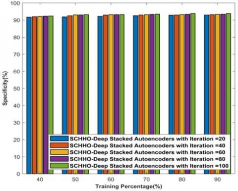
Figure 4 portrays analysis of proposed SCHHO-Deep stacked Auto-encoders based on training data using accuracy, sensitivity and specificity parameters. The analysis of proposed SCHHO-Deep stacked Auto-encoders considering accuracy parameter is described in Fig 4a). For 40% training data, the accuracies computed by proposed SCHHO-Deep stacked Auto-encoders with 20 iterations, 40 iterations, 60 iterations, 80 iteration and 100 iterations are, 88.782%, 89.698%, 91.265%, 91.625%, and 91.671%. Likewise, for 90% training data, the corresponding accuracies computed by proposed SCHHO-Deep stacked Auto-encoders with 20 iterations, 40 iterations, 60 iterations, 80 iteration and 100 iterations are 94.333%, 94.374%, 94.379%, 94.422%, 94.939%. Analysis of proposed SCHHO-Deep stacked Auto-encoders considering sensitivity parameter is described in Fig 4b). For 40% training data, the sensitivities computed by proposed SCHHO-Deep stacked Auto-encoders with 20 iterations, 40 iterations, 60 iterations, 80 iteration and 100 iterations are 85.282%, 85.325%, 85.626%, 85.801%, and 85.937%. Likewise, for 90% training data, the corresponding sensitivities computed by proposed SCHHO-Deep stacked Auto-encoders with 20 iterations, 40 iterations, 60 iterations, 80 iteration and 100 iterations are 86.037%, 89.015%, 89.809%, 89.942%, and 91.194%. Analysis of proposed SCHHO-Deep stacked Auto-encoders considering specificity parameter is described in Fig 4c). For 40% training data, the specificities computed by proposed SCHHO-Deep stacked Auto-encoders with 20 iterations, 40 iterations, 60 iterations, 80 iteration and 100 iterations are 91.686%, 91.983%, 92.149%, 92.297%, and 92.398%. Likewise, for 90% training data, the corresponding specificities computed by proposed SCHHO-Deep stacked Auto-encoders with 20 iterations, 40 iterations, 60 iterations, 80 iteration and 100 iterations are 92.972%, 93.169%, 93.342%, 93.411%, and 93.845%.
We tried to find the time complexity for training a neural network that has 12 layers with respectively h, i, j, k, l, m, n, o, p, q, r and s nodes, with t training examples and e epochs. The result was O(et∗(hi+ij+jk+kl+lm+mn+no+op+pq+qr+rs)).
(a) Accuracy
(b) Sensitivity
(c) Specificity
Figure 4. SCHHO-Deep stacked Auto-encoders based on training data
4.6.2 Analysis based on K-Fold
(a) Accuracy
(b) Sensitivity
(c) Specificity
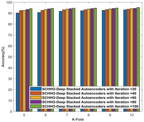
Figure 5. Analysis of proposed SCHHO-Deep stacked Auto-encoders based on K-Fold
The procedure has a single parameter called k that refers to the number of groups that a given data sample is to be split into. As such, the procedure is often called k-fold cross-validation. In each set (fold) training and the test would be performed precisely once during this entire process. It helps us to avoid overfitting. To achieve this K-Fold Cross Validation, we have to split the data set into two sets, Training and Testing with the challenge of the volume of the data. We have use K=5 for K fold cross validation.
Figure 5 portrays analysis of proposed SCHHO-Deep stacked Auto-encoders based on K-Fold using accuracy, sensitivity and specificity parameters. The analysis of proposed SCHHO-Deep stacked Auto-encoders considering accuracy parameter is described in Figure 5a). For K-Fold=5, the accuracies computed by proposed SCHHO-Deep stacked Auto-encoders with 20 iterations, 40 iterations, 60 iterations, 80 iteration and 100 iterations are 90.151%, 92.405%, 92.557%, 93.385%, and 94.117%. Likewise, for K-Fold=10, the corresponding accuracies computed by proposed SCHHO-Deep stacked Auto-encoders with 20 iterations, 40 iterations, 60 iterations, 80 iteration and 100 iterations are 93.062%, 93.641%, 94.122%, 94.365%, and 95.159%. From the Figure 5 (a) the convergence of SCHHO algorithm is 92% for 60 iterations and with increase in number of iteration from 60 to 100 the accuracy of SCHHO algorithm is nearly same as with the increase in additional training the model is not improving. Analysis of proposed SCHHO-Deep stacked Auto-encoders considering sensitivity parameter is described in Figure 5b). For K-Fold=5, the sensitivities computed by proposed SCHHO-Deep stacked Auto-encoders with 20 iterations, 40 iterations, 60 iterations, 80 iteration and 100 iterations are 85.239%, 85.265%, 85.365%, 85.405%, and 85.448%. Likewise, for K-Fold=10, the corresponding sensitivities computed by proposed SCHHO-Deep stacked Auto-encoders with 20 iterations, 40 iterations, 60 iterations, 80 iteration and 100 iterations are 88.928%, 89.167%, 89.397%, 89.747%, and 90.157%. The analysis of proposed SCHHO-Deep stacked Auto-encoders considering specificity parameter is described in Figure 5c). For K-Fold=5, the specificities computed by proposed SCHHO-Deep stacked Auto-encoders with 20 iterations, 40 iterations, 60 iterations, 80 iteration and 100 iterations are 92.766%, 93.273%, 93.325%, 93.362%, and 93.592%. Likewise, for K-Fold=10, the corresponding specificities computed by proposed SCHHO-Deep stacked Auto-encoders with 20 iterations, 40 iterations, 60 iterations, 80 iteration and 100 iterations are 93.486%, 93.534%, 93.624%, 93.641%, and 93.761%.
4.7 Comparative analysis
In terms of accuracy, sensitivity, and specificity, SCHHO-Deep stacked Auto-encoders are compared to traditional approaches. Variating training data and K-Fold performs the analysis.
4.7.1 Analysis based on training data
(a) Accuracy
(b) Sensitivity
(c) Specificity
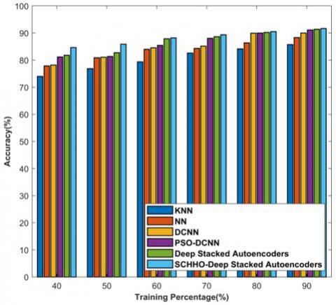
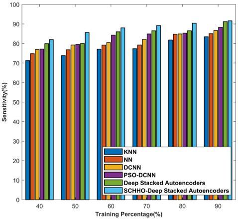
Figure 6. Analysis of methods based on training data
Figure 6 shows the accuracy, sensitivity, and specificity of suggested SCHHO-Deep stacked Auto-encoders. Figure 6a) analyses strategies based on accuracy. For 40% training data, the accuracies computed by KNN, NN, Deep CNN, PSO-Deep CNN, Deep stacked Auto-encoders, and Proposed SCHHO-Deep stacked Auto-encoders are 74.002%, 77.863%, 78.194%, 81.182%, 81.795%, and 84.618%. Likewise, for 90% training data, the corresponding accuracies computed by KNN, NN, Deep CNN, PSO-Deep CNN, Deep stacked Auto-encoders, and Proposed SCHHO-Deep stacked Auto-encoders are 85.715%, 88.320%, 90.005%, 91.104%, 91.364%, and 91.669%. The analysis of methods considering sensitivity parameter is described in Figure 6b). For 40% training data, the sensitivities computed by KNN, NN, Deep CNN, PSO-Deep CNN, Deep stacked Auto-encoders, and Proposed SCHHO-Deep stacked Auto-encoders are 71.258%, 74.804%, 76.924%, 77.162%, 79.921%, and 81.975%. Likewise, for 90% training data, the corresponding sensitivities computed by KNN, NN, Deep CNN, PSO-Deep CNN, Deep stacked Auto-encoders, and Proposed SCHHO-Deep stacked Auto-encoders are 83.465%, 85.042%, 86.660%, 88.359%, 91.188%, and 91.610%. The analysis of proposed SCHHO-Deep stacked Auto-encoders considering specificity parameter is described in Figure 6c). For 40% training data, the specificities computed by KNN, NN, Deep CNN, PSO-Deep CNN, Deep stacked Auto-encoders, and Proposed SCHHO-Deep stacked Auto-encoders are 83.716%, 84.773%, 85.126%, 85.203%, 85.428% and 86.155%. Likewise, for 90% training data, the corresponding specificities computed by KNN, NN, Deep CNN, PSO-Deep CNN, Deep stacked Auto-encoders, and Proposed SCHHO-Deep stacked Auto-encoders are 90.445%, 90.922%, 91.109%, 91.529%, 91.540%, and 91.728%.
4.7.2 Analysis based on K-Fold
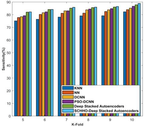
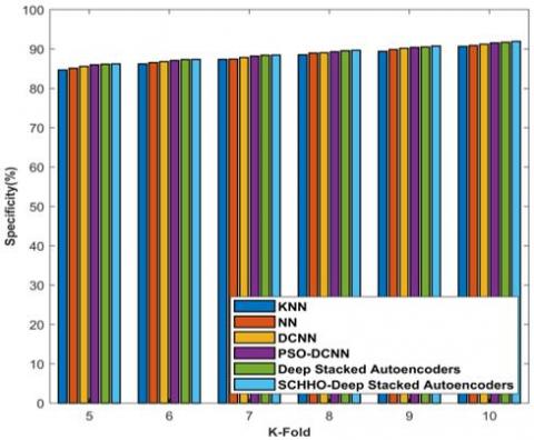
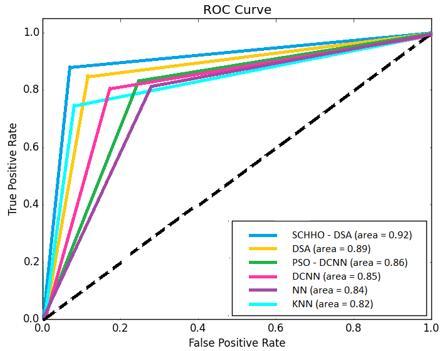
Figure 7 demonstrates K-Fold accuracy, sensitivity, and specificity analyses. Figure 7a) analyses strategies based on accuracy. For K-Fold=5, the accuracies computed by KNN, NN, Deep CNN, PSO-Deep CNN, Deep stacked Auto-encoders, and Proposed SCHHO-Deep stacked Auto-encoders are 77.471%, 80.278%, 84.110%, 84.174%, 85.009%, and 85.929%. Likewise, for K-Fold=10, the corresponding accuracies computed by KNN, NN, Deep CNN, PSO-Deep CNN, Deep stacked Auto-encoders, and Proposed SCHHO-Deep stacked Auto-encoders are 84.092%, 87.085%, 89.747%, 90.406%, 91.069%, and 91.216%. The analysis of methods considering sensitivity parameter is described in Fig 7b). For K-Fold=5, the sensitivities computed by KNN, NN, Deep CNN, PSO-Deep CNN, Deep stacked Auto-encoders, and Proposed SCHHO-Deep stacked Auto-encoders are 75.101%, 7.779%, 78.417%, 79.212%, 82.004%, and 82.204%. Likewise, for K-Fold=10, the corresponding sensitivities computed by KNN, NN, Deep CNN, PSO-Deep CNN, Deep stacked Auto-encoders, and Proposed SCHHO-Deep stacked Auto-encoders are 82.250%, 83.996%, 85.176%, 86.661%, 87.805%, and 88.900%. The analysis of methods considering specificity parameter is described in Figure 7c). For K-Fold=5, the specificities computed by KNN, NN, Deep CNN, PSO-Deep CNN, Deep stacked Auto-encoders, and Proposed SCHHO-Deep stacked Auto-encoders are 84.673%, 85.106%, 85.565%, 85.977%, 86.144%, and 86.217%. Likewise, for K-Fold=10, the corresponding specificities computed by KNN, NN, Deep CNN, PSO-Deep CNN, Deep stacked Auto-encoders, and Proposed SCHHO-Deep stacked Auto-encoders are 90.674%, 90.874%, 91.196%, 91.540%, 91.689%, and 91.912%. Figure 8 shows ROC – AUC of algorithms.
4.8 Comparative discussion
Table 2 illustrates comparative analysis of approaches using accuracy, sensitivity and specificity parameter. Based on the training data, accuracy of proposed SCHHO-Deep stacked Auto-encoders is 91.669%, accuracy of Deep stacked Auto-encoders is 91.364%, which is lesser than the proposed method. The sensitivity of proposed SCHHO-Deep stacked Auto-encoders is 91.610, whereas the specificity of proposed SCHHO-Deep stacked Auto-encoders is 91.728%. SCHHO-Deep stacking Auto-encoder has 91.216 % accuracy, 88.900 % sensitivity, and 91.912 % specificity for K-Fold values.
(a) Accuracy
(b) Sensitivity
(c) Specificity
Figure 7. Analysis of methods based on K-Fold
Figure 8. ROC – AUC of algorithms
Table 2. Comparative analysis
|
Variation |
Metrics |
KNN |
NN |
Deep CNN |
PSO- Deep CNN |
Deep stacked Auto-encoders |
Proposed SCHHO- Deep stacked Auto-encoders |
|
Training data |
Accuracy |
85.715 |
88.320 |
90.005 |
91.104 |
91.364 |
91.669 |
|
Sensitivity |
83.465 |
85.042 |
86.660 |
88.359 |
91.188 |
91.610 |
|
|
Specificity |
90.445 |
90.922 |
91.109 |
91.529 |
91.540 |
91.728 |
|
|
K-Fold |
Accuracy |
84.092 |
87.085 |
89.747 |
90.406 |
91.069 |
91.216 |
|
Sensitivity |
82.250 |
83.996 |
85.176 |
86.661 |
87.805 |
88.900 |
|
|
Specificity |
90.674 |
90.874 |
91.196 |
91.540 |
91.689 |
91.912 |
In this research, fully automated, deep stacked auto encoder is proposed for detection of skin lesions. Autoencoders are beneficial when you have a small dataset because they can learn to compress your data into a lower-dimensional space. Deep stacked auto encoder is trained using suggested SCHHO. The SCA and HHO algorithms were combined to create the suggested SCHHO algorithm, which can be used to establish excellent skin cancer diagnosis by determining the ideal weights. Segmentation step is performed on each input skin image utilizing Sparse FCM algorithm. Skin lesion regions’ most pertinent pixels aid in better segmentation outcomes. For the accurate detection of skin lesions, statistical and textural features are also used. Because of the preprocessing step that offers opportunity to enhance outcomes even when using low quality photographs, the approach can be modified to improve image quality. With maximum accuracy of 91.669 %, maximum sensitivity of 91.610 %, and maximum specificity of 91.728 %, respectively, the suggested SCHHO-Deep stacked auto-encoder surpassed other approaches. Other skin cancer datasets will be used in future to calculate effectiveness of suggested strategy. Advanced optimization methods will also be studied to increase effectiveness of current approaches. Autoencoders are often trained with a single layer encoder and a single layer decoder, but using many-layered (deep) encoders and decoders offers many advantages. Depth can exponentially reduce the computational cost of representing some functions. Depth can exponentially decrease the amount of training data needed to learn some functions. Experimentally, deep autoencoders yield better compression compared to shallow or linear autoencoders.
[1] Khan, M.Q., Hussain, A., Rehman, S.U., Khan, U., Maqsood, M., Mehmood, K., Khan, M.A. (2019). Classification of melanoma and nevus in digital images for diagnosis of skin cancer. IEEE Access, 7: 90132-90144. https://doi.org/10.1109/ACCESS.2019.2926837
[2] Conoci, S., Rundo, F., Petralta, S., Battiato, S. (2017). Advanced skin lesion discrimination pipeline for early melanoma cancer diagnosis towards PoC devices. In 2017 European Conference on Circuit Theory and Design (ECCTD), Catania, Italy, pp. 1-4. https://doi.org/10.1109/ECCTD.2017.8093310
[3] Nezhadian, F.K., Rashidi, S. (2017). Melanoma skin cancer detection using color and new texture features. In 2017 Artificial Intelligence and Signal Processing Conference (AISP), pp. 1-5. https://doi.org/10.1109/AISP.2017.8324108
[4] Sahu, P., Yu, D., Qin, H. (2018). Apply lightweight deep learning on internet of things for low-cost and easy-to-access skin cancer detection. In Medical Imaging 2018: Imaging Informatics for Healthcare, Research, and Applications, 10579: 254-262. https://doi.org/10.1117/12.2293350
[5] Kawahara, J., Daneshvar, S., Argenziano, G., Hamarneh, G. (2018). Seven-point checklist and skin lesion classification using multitask multimodal neural nets. IEEE Journal of Biomedical and Health Informatics, 23(2): 538-546. https://doi.org/10.1109/JBHI.2018.2824327
[6] Serte, S., Demirel, H. (2019). Gabor wavelet-based deep learning for skin lesion classification. Computers in Biology and Medicine, 113: 103423. https://doi.org/10.1016/j.compbiomed.2019.103423
[7] Zhao, X.Y., Wu, X., Li, F.F., Li, Y., Huang, W.H., Huang, K., ... & Zhao, S. (2019). The application of deep learning in the risk grading of skin tumors for patients using clinical images. Journal of Medical Systems, 43(8): 1-7. https://doi.org/10.1007/s10916-019-1414-2
[8] Albahar, M.A. (2019). Skin lesion classification using convolutional neural network with novel regularizer. IEEE Access, 7: 38306-38313. https://doi.org/10.1109/ACCESS.2019.2906241
[9] Celebi, M.E., Kingravi, H.A., Uddin, B., Iyatomi, H., Aslandogan, Y.A., Stoecker, W.V., Moss, R.H. (2007). A methodological approach to the classification of dermoscopy images. Computerized Medical Imaging and Graphics, 31(6): 362-373. https://doi.org/10.1016/j.compmedimag.2007.01.003
[10] Walvick, R.P., Patel, K., Patwardhan, S.V., Dhawan, A.P. (2004). Classification of melanoma using wavelet transform-based optimal feature set. In Medical Imaging 2004: Image Processing, 5370: 944-951. https://doi.org/10.1117/12.536013
[11] Nimunkar, A., Dhawan, A.P., Relue, P.A., Patwardhan, S.V. (2002). Wavelet and statistical analysis for melanoma classification. In Medical Imaging 2002: Image Processing, 4684: 1346-1353. https://doi.org/10.1117/12.467098
[12] Maglogiannis, I., Doukas, C.N. (2009). Overview of advanced computer vision systems for skin lesions characterization. IEEE Transactions on Information Technology in Biomedicine, 13(5): 721-733. https://doi.org/10.1109/TITB.2009.2017529
[13] Breiman, L. (2001). Random forests. Machine Learning, 45(1): 5-32. https://doi.org/10.1023/a:1010933404324
[14] Landwehr, N., Hall, M., Frank, E. (2005). Logistic model trees. Machine Learning, 59(1): 161-205. https://doi.org/10.1007/s10994-005-0466-3
[15] Burlina, P.M., Joshi, N.J., Ng, E., Billings, S.D., Rebman, A.W., Aucott, J.N. (2019). Automated detection of erythema migrans and other confounding skin lesions via deep learning. Computers in Biology and Medicine, 105: 151-156. https://doi.org/10.1016/j.compbiomed.2018.12.007
[16] Pandey, P., Saurabh, P., Verma, B., Tiwari, B. (2019). A multi-scale retinex with color restoration (MSR-CR) technique for skin cancer detection. In Soft Computing for Problem Solving, pp. 465-473. https://doi.org/10.1007/978-981-13-1595-4_37
[17] Tan, T.Y., Zhang, L., Lim, C.P. (2019). Intelligent skin cancer diagnosis using improved particle swarm optimization and deep learning models. Applied Soft Computing, 84: 105725. https://doi.org/10.1016/j.asoc.2019.105725
[18] Dorj, U.O., Lee, K.K., Choi, J.Y., Lee, M. (2018). The skin cancer classification using deep convolutional neural network. Multimedia Tools and Applications, 77(8): 9909-9924. https://doi.org/10.1007/s11042-018-5714-1
[19] Saba, T., Khan, M.A., Rehman, A., Marie-Sainte, S.L. (2019). Region extraction and classification of skin cancer: A heterogeneous framework of deep CNN features fusion and reduction. Journal of Medical Systems, 43(9): 1-19. https://doi.org/10.1007/s10916-019-1413-3
[20] Patil, R., Bellary, S. (2021). Transfer learning based system for melanoma type detection. Revue d'Intelligence Artificielle, 35(2): 123-130. https://doi.org/10.18280/ria.350203
[21] Patil, R., Bellary, S. (2020). Machine learning approach in melanoma cancer stage detection. Journal of King Saud University-Computer and Information Sciences. https://doi.org/10.1016/j.jksuci.2020.09.002
[22] Patil, R. (2021). Machine learning approach for malignant melanoma classification. International Journal of Science, Technology, Engineering and Management-A VTU Publication, 3(1): 40-46.
[23] Patil, R., Bellary, S. (2021). Ensemble Learning for Detection of Types of Melanoma. In 2021 International Conference on Computing, Communication and Green Engineering (CCGE), pp. 1-6. https://doi.org/10.1109/CCGE50943.2021.9776373
[24] Chang, X., Wang, Q., Liu, Y., Wang, Y. (2016). Sparse Regularization in Fuzzy c-Means for High-Dimensional Data Clustering. IEEE Transactions on Cybernetics, 47(9): 2616-2627. https://doi.org/10.1109/TCYB.2016.2627686
[25] Chakraborti, T., McCane, B., Mills, S., Pal, U. (2017). LOOP descriptor: Encoding repeated local patterns for fine-grained visual identification of lepidoptera. arXiv preprint arXiv:1710.09317, 1-5.
[26] Jayapriya, K., Mary, N. (2019). Employing a novel 2-gram subgroup intra pattern (2GSIP) with stacked auto encoder for membrane protein classification. Molecular Biology Reports, 46(2): 2259-2272. https://doi.org/10.1007/s11033-019-04680-3
[27] Skin cancer dataset. (2019). https://challenge2019.isic-archive.com/data.html
[28] Linsangan, N.B., Adtoon, J. (2018). Skin cancer detection and classification for moles using k-nearest neighbor algorithm. In Proceedings of the 2018 5th International Conference on Bioinformatics Research and Applications, pp. 47-51. https://doi.org/10.1145/3309129.3309141
[29] Jianu, S. R. S., Ichim, L., Popescu, D. (2019). Automatic diagnosis of skin cancer using neural networks. In 2019 11th International Symposium on Advanced Topics in Electrical Engineering (ATEE), pp. 1-4. https://doi.org/10.1109/ATEE.2019.8724938
[30] Chang, X., Wang, Q., Liu, Y., Wang, Y. (2016). Sparse Regularization in Fuzzy c-Means for High-Dimensional Data Clustering. IEEE Transactions on Cybernetics, 47(9): 2616-2627. https://doi.org/10.1109/TCYB.2016.2627686