Safia Djemame* | Siham Fichouche
© 2022 IIETA. This article is published by IIETA and is licensed under the CC BY 4.0 license (http://creativecommons.org/licenses/by/4.0/).
OPEN ACCESS
Edge detection is a key technique in image processing. The detected edge quality has a direct and significant impact on performance. There is a multitude of methods for edge detection but they are strongly associated with the application and the quality of the images. However, more precise outcomes and a reduced execution time remain the primary objectives for extracting edges. To address these issues, we propose a novel technique based on a complex system called Cellular Automata (CA). They are successfully applied in edge detection due to their simplicity and local interactions. This undertook shed new light on a novel method using Outer Totalistic Cellular Automata (OTCA) to perform efficiently edge detection. We have tested images from Berkeley dataset. RMSE and SSIM are used as fitness functions for estimating numerical performance of OTCA rules. Comparisons were made with classical edge detectors like: Canny, Scharr, Sobel, Roberts. Experimental results showed that OTCA rules provide excellent performance and outperforms other edge detectors in terms of precision and execution time, particularly when dealing with noisy images.
image processing, edge detection, cellular automata, transition rule, rule optimization
Image processing is one of the key factors influencing the research progress and it is deeply motivated to be a driving force in the technology race. It rivals human visual abilities and brings significant benefits in many areas. In image processing, edge detection is a crucial stage. The image edge is the most visible portion of the partial intensity fluctuations in pictures [1] that define the borders of objects in a scene. It is a primary step in image processing, image analysis, pattern identification in images, computer vision, and human vision. The objective of detecting abrupt changes in the brightness of an image is to capture significant events and features. By using an edge detector on an image, you may considerably lessen the amount of data that has to be processed and thereby filter out information that is deemed less important while keeping the image's crucial structural qualities [2]. The merits of detected edges algorithms have a direct and high influence on system performance. The accuracy and dependability of its outputs have a direct effect on the objective world comprehension machine system.
It is challenging to create a general-purpose edge detection algorithm that performs effectively in a wide variety of situations and meets the needs of later processing stages. As a result, throughout the history of digital image processing, several edge detectors have been developed, each with a specific features and mathematical and algorithmic qualities [3].
There are several edge detection methods, but the majority of them fall into two categories: search-based and zero-crossing-based [4]. The search-based methods for detecting edges begin by computing a measure of edge strength, typically a first-order derivative expression such as the gradient magnitude, and then searching for local directional maxima of the gradient magnitude using a computed estimate of the edge's local orientation, usually the gradient direction (Canny [5], Deriche [6]). Biological vision has a significant effect on edge identification based on second-order difference (zero crossings). Marr and Hildreth [7] and Marr [8] discuss the pioneering work.
Each technique of image edge detection has distinct benefits and limitations, and further study is needed to develop algorithms to increase the use of edge detection not just for higher level image processing, but also for accuracy. To accomplish this purpose, the following investigations are necessary:
Numerous standard methods for the majority of image processing problems have already been created over the previous few decades by various researchers. Their concern is always to improve the quality of the expected result while reducing the processing time. In recent years, much effort has been expended on developing other techniques of edge detection. In this context, several academics have examined the capacity of cellular automata to handle the same issue and discovered that it outperforms conventional techniques. There has been increasing interest in the last decade in employing cellular automata to accomplish edge detection.
Due to the parallel nature of cellular automata (CA), they have become an interesting topic of research for academics from a wide range of domains. They are utilized in engineering and science areas. The appeal of cellular automata can be attributed to their simplicity and, despite its inherent parallelism, their immense potential for representing complex systems [9]. It’s found to be efficient in several image processing tasks, regarding grid structure, local interactions, emerging behavior, and low time processing.
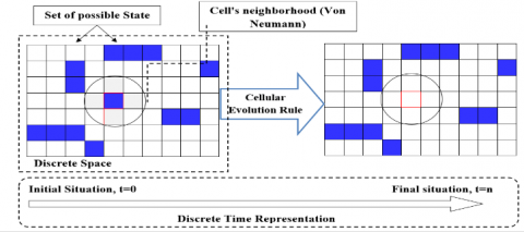
Cellular Automata expressed by an n-dimensional array of cells. Each cell starts from an initial to a final state. All cells are updated in discrete stages synchronously according to a basic local rule. Each cell's current state is determined by its previous state and the states of its nearest neighbors. The primary advantage of CA is that each cell normally adheres to a few basic principles; but, when a matrix of cells is combined with their local interaction, more intricate emergent global behavior occurs.
Numerous variants of CA have been presented by various researchers to facilitate the design and simulation of complex systems: uniform, hybrid, null boundary, periodic boundary, linear, nonlinear, complement, additive…etc. [10]. Each of these types of CA has shown varied and amazing advantages and properties, it has also opened the horizon to future explorations for the use of CA in different areas. The related literature that will be detailed in the following paragraph will present a variety of CA models used for image processing.
However, it has been found that the kind of CA called Outer Totalistic Cellular Automata (OTCA) has been rarely used, this encouraged us to explore its capabilities and high complexity to carry out edge detection. Likewise, a comparative study assesses their relative merit over classical methods of edge detection: Canny, Sobel, Prewitt, Roberts and Scharr. Visual inspection and statistical evaluation consolidate the promising results obtained by the OTCA rules.
A two-dimensional array of (n x m) pixels is referred to as a digital image. Each pixel is denoted by the triplet (i, j, k), where (i, j) identifies its array position and k is the associated color. The image may thus be regarded as a particular configuration state of a cellular automaton with the (n x m) array defined by the image as its cellular space. Each cell in the array represents a single pixel. The cell state is the pixel intensity. This projection makes the CA model an interesting tool to perform digital image processing tasks. Moreover, due to their local character and straightforward parallel computation implementation, cellular automata appear to be ideal instruments for image processing. Numerous research studies have been conducted in this field to train cellular automata for image processing applications.
Several algorithms for edge detection have been developed, such as Sobel [11], Prewitt [12], and Canny [13], obtaining adequate edge extraction at a desirable level of performance remains a difficult issue.
Rosin [14] demonstrates the possibility of learning effective rule sets for basic image processing applications, as well as numerous variations to the classic CA formulation. Also, he described the application of CA for various image processing tasks in Ref. [15]. Preston and Duff [16] provided a single source, detailed descriptions of exact CA machines, assembling such work and demonstrating the range and efficacy of CA-based methods to image processing challenges. Diosan et al. [17] presented in detail a class of CA applied for image processing tasks. In the last few decades, numerous standard methods have previously been established by various academics for the majority of image processing applications. However, other researchers eventually discovered that using CA to tackle the identical problem was superior [2]. Enhancing accuracy of the edges, and less time consuming remains challenging problems.
In the literature, there are a lot of works based on CA models for performing edge detection [2]. We cite:
- Wongthanavasu et al. [18] presented a uniform CA rule based on the Von Neumann neighborhood for edge detection on binary and gray-scale images;
- Chang et al. [19] presented CA edge detection model. The gray scale matrix of the image was dealt with using an information orientation approach, a new kind of CA neighborhood was established, and an appropriate local rule of the CA was designed;
- Ha [20] introduced a nonlinear CA-based approach for edge detection. Experiments have demonstrated that the novel edge detection approach successfully eliminates noise and assures the continuity, integrity, and precise position of edges;
- Ke et al. [21] improved the edge detection technique based on the cloud model CA. It combines direction and edge order information to create cloud seasoning, then provides feedback to the input data and detects auto evolution through CA;
- Liu et al. [22] adopted a two-dimensional fuzzy CA model, a quadrangle-shaped grid, and maximin law as the conversion rule for the fuzzy cellular automata;
- Kumar et al. [23] proposed an optimal approach for edge detection based on CA;
- Djemame and Batouche [24] proposed a new edge detection algorithm, based on CA to extract edges of different types of images, using a totalistic transition rule. They used a meta-heuristic, Particle Swarm Optimization, to determine the most optimum and acceptable set of CA transition rules for the edge detection task;
- Zagoris et al. [25] suggested a method for recognizing scene in natural photos; to begin, a binary edge map is constructed using the CA's flexibility; subsequent phases include the application of altering transition rules;
- Dhillon [26] presented a robust CA approach based on edge detection. The simulation results indicate that the suggested approach detects edges more smoothly and in less time than other edge detectors;
- Priego et al. [27] deals with the problem of finding edges in hyperspectral images. For this purpose, he utilized cellular automata (CA) and their advantageous emergent behavior;
- Gorsevski et al. [28] explored the application of two-dimensional CA to the challenge of detecting and extracting grain boundaries from digital images of thin slices in damaged rocks;
- Uguz et al. [29] suggested an efficient and straightforward approach for edge identification using a uniform CA transition matrix format. Sahin et al. [30] described a solution for edge detection thresholding that is based on fuzzy CA transition rules tuned with the Particle Swarm Optimization metaheuristic. Diwakar et al. [31] employed CA-based edge detection to detect malignant cells in the brain. They adopted CA guidelines to assist in assessing the tumor's precise location and size;
- Rosin and Sun [32] discussed the advantages and disadvantages of CA-based edge detection approaches and evaluated their respective qualities and limitations. Numerous CA-based edge detection algorithms are implemented and evaluated in order to provide a baseline comparison of competing approaches;
- Mohammed and Nayak [3] proposed a novel pattern of two-dimensional CA linear rules that might be employed for image edge identification. Each suggested rule detects edges more accurately than existing edge detection methods when an image is enhanced;
- Mofrad et al. [33] introduced a novel CA local rule with adaptive neighborhood type to generate an image's edge map, in comparison to CA with a fixed neighborhood;
- Han et al. [34] took into account the space computing capacity of CA and the data pattern search capability of Extreme Learning Machine and proposed an extreme learning machine for edge identification in remote sensing images based on CA;
- Amrogowicz et al. [35] pioneered the use of Outer Totalistic CA to create a distinctive edge detector. The most significant distinctions between their work and our study are as follows:
* The fitnesses: we used SSIM and RMSE functions while [35] employed Pratt FOM,
* The selected rules are different,
* The data-set held for test and comparison: we used Berkeley dataset, while [35] employed (USF) Florida dataset,
* For the visualization of testing images, [35] used one single image, while we presented a large variety of images for illustrating our results,
* In ref. [35], we noticed a lack of statistical evaluation for images without noise.
- Aghaei [36] proposed a system for noisy image edge identification based on a four-neighborhood under Null Boundary CA for noise removal and a two-dimensional twenty-five neighborhood under Null Boundary CA for edge detection;
- Enescu et al. [37] demonstrated the compatibility and capacity of CA in image processing tasks by presenting an edge identification approach for binary images based on CA and Evolutionary Algorithms.
Other researchers proposed to solve image processing tasks with CA optimizing rules by the use of metaheuristics. Kazar and Slatnia [38] utilized a genetic algorithm to identify a set of rules for edge detection. A genetic algorithm is an evolutionary process that continuously evolves CA to get the best edge detection.
Djemame et al. [39] used a QPSO algorithm to evolve cellular automata for edge detection and noise filtering.
Djemame and Batouche [40] suggest using Quantum Genetic Algorithms (QGA) to train Cellular Automata for edge detection tasks.
Based on previous research results, we propose a new approach of edge detection using a class of CA called: Outer Totalistic Cellular Automata (OTCA). New rules are extracted, and trained on a benchmark of images. Therefore, we validate and compare the results with several existing edge detectors. Our results are produced very quickly. The results are compared with well-known edge detectors. Performance results are also calculated.
3.1 Definition
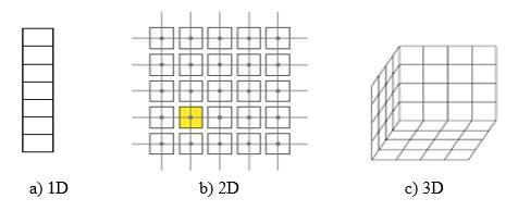
CAs are composed of a regular grid of locally linked finite state machines, or cells, which update their states in response to their immediate neighbors and a predefined updating transition rule [3]. The grid may have any number of dimensions, and all of the cells' states are changed concurrently (Figure 1).
Figure 1. Example of CA Cells representation
3.2 Characteristics of Cellular Automata
Cellular Automata are available in a variety of forms and configurations. They are defined by four characteristics [11]:
3.2.1 The Lattice Geometry
This can be a D-dimensional (possibly infinite) grid (Figure 2). It is the most fundamental properties of a CA on which it is computed.
Figure 2. Schematic diagram of CA
3.2.2 State of Cellular Automata
At each time step, the transition rules are applied, and the future state of each cell is decided by the present state of its nearby cells [13].
3.2.3 Neighborhood Structure
Neighborhood configuration is an essential element of CA model. There are different neighborhood structures. In the case of a two-dimensional cellular automaton on a square grid, two frequently encountered neighborhoods are the Moore neighborhood (a square neighborhood) and the Von Neumann neighborhood (a diamond-shaped neighborhood) (Figure 3) [10].
Figure 3. Examples of CA neighborhoods [10]
3.2.4 Transition Rule
The transition rules determine the changing state of a cell depending on the lattice geometry, the neighborhood, and the state set [3]. Additionally, the nature of future state functions varies greatly; researchers have created the rule set in accordance with the application's design needs.
Moreover, rules are distributed globally during each time step, and the next state of each cell is decided by the present state of its nearby cells.
This section introduces the OTCA-based edge detector. CA is an effective way to model a picture in image processing. A cell's state is determined by the pixel's color. The transition rule is specified by the cell's current state and the neighborhood's current state. The input picture to be processed is the starting configuration of CA, and the output image is the final configuration (segmented and filtered). The CA progresses from a known beginning configuration to a final global state utilizing a limited subset of rules across successive iterations. Fitness functions are used to evaluate the quality of the produced edge visually and statistically.
4.1 The model
The suggested technique employs a rectangular, two-dimensional grid L for image processing, with each cell representing one pixel in the image. Each cell has a limited number of discrete states S = {0, 1,..., k-1}. The grid's initial values match to the values in image $S_{0} \in S$. Each cell updates its state concurrently in discrete time steps according to a transition rule based on its local neighborhood N. We employ an outer totalistic transition rule in this study. It is discussed in further detail in the next paragraph.
4.2 Outer Totalistic Cellular Automata
Wolfram came up with the concept of a totalistic CA. It is a CA whose rules are determined only by the total of the values of the cells in a neighborhood, including the core cell. In OTCA, the next cell state is determined only by the total of neighboring cells (not including the central cell) and the value of the center cell [9].
The rule number is given by defining the next cell state as a binary string based on the sum of cells in the neighborhood. There are precisely 210 = 1024 possible rules for a Moore neighborhood in Totalistic Cellular Automata, where the total might be between 0 and 9. The binary string for the Totalistic rule 56 is shown in Table 1, in which the next state of the center cell becomes 1 when the total of the neighboring values is between 3 and 5.
Table 1. Totalistic rule 56
|
Neighborhood sum |
9 |
8 |
7 |
6 |
5 |
4 |
3 |
2 |
1 |
0 |
|
Next state |
0 |
0 |
0 |
1 |
1 |
1 |
1 |
0 |
0 |
0 |
In contrast to traditional TCA, the state of the central cell has a considerable effect on the subsequent state. Because two transitions based on the center pixel must be defined for each sum of neighborhoods, the search space becomes significantly bigger. For a Moore neighborhood, the total can range from 0 to 8, resulting in 18 unique patterns and 218 = 262144 potential rules. Table 2 illustrates OTCA rule 832. The next state of the cell is '1' if the total is 3 and the central pixel is '0', and '4' if the sum is 3 and the central pixel is '0' regardless of the central pixel state.
Table 2. Outer Totalistic rule 832
|
Neighborhood sum |
8 |
7 |
6 |
5 |
4 |
3 |
2 |
1 |
0 |
|||||||||
|
Central pixel value |
1 |
0 |
1 |
0 |
1 |
0 |
1 |
0 |
1 |
0 |
1 |
0 |
1 |
0 |
1 |
0 |
1 |
0 |
|
Next state |
0 |
0 |
0 |
0 |
0 |
0 |
0 |
0 |
1 |
1 |
0 |
1 |
0 |
0 |
0 |
0 |
0 |
0 |
4.3 Rule selection
Rules are reprogrammable micro-programs that may be launched in response to any detected condition or at the push of a button. In CA, rules determine how the infinite arrangement of cells will be updated from time step to another. Time is split into discrete steps, and the rules define how to determine a cell's next state depending on its present state and its surroundings. All cells repeatedly apply the rule; this recursive application results in CA's extraordinary behaviour.
CA rules may identify relatively strong fluctuations in image brightness, colour, or detail and can locate edges using this extracted information [33]. With such a huge search space, manual rule selection would be challenging and might result in the exclusion of potentially significant rules. Thus, a thorough survey of the rule space is required to arrive at an optimal result [35].
Consider the Moore Neighbourhood as a binary picture. The whole number of OTCA rules can be thoroughly iterated with the quality metric computation in a reasonable amount of time; certain rules can be deleted beforehand. The first and last pieces of the rule string denote a uniform neighbourhood, which is denoted by the absence of an edge. The second bit and the one before it reflects the presence of a noise pixel in the center. By specifying a value for each of the four stated cases, the number of viable rules is decreased from 262144 to 16384, saving 93.75 % of the time spent searching.
4.4 Fitness functions
With a total of 16384 rules remaining, it is difficult to visually check the optimal rule. It is necessary to select a well-defined metric for quantitative evaluation. Despite the obvious benefits of a unified quantitative approach, no agreement has been reached and several alternative measures have been offered. Whichever optimization approach is employed, an objective function is necessary, and the quality of the objective function obviously has a significant impact on the final outcomes. Two fitness functions were considered: the Structural Similarity Index (SSIM) and the Root Mean Square Error (RMSE). These functions are used to determine the difference in picture quality between the generated image and the reference image. For each test picture, the RMSE and SSIM values were determined.
4.4.1 The Root Mean Square Error
The Root Mean Square Error (RMSE) is a widely used metric for comparing expected values by a model or estimator to observed values. The RMSE is used to aggregate the magnitudes of prediction errors across many time periods into a single measure of predictive capacity. It is a measure of accuracy between the original and distorted images. Eq. (1) calculates the RMSE value.
$R M S E=\sqrt{\frac{1}{n_{x} n_{y}} \sum_{0}^{n_{x}-1} \sum_{0}^{n_{y}-1}[E(x, y)-O(x, y)]^{2}}$ (1)
where:
4.4.2 The Structural Similarity Index
The Structural Similarity Index (SSIM) aims to assess the visually discernible difference between a distorted image and a reference image. The method defines structural information in a picture as those qualities that accurately describe the structure of the objects in the scene, regardless of their average brightness or contrast. The index is calculated by comparing brightness, contrast, and structure. The comparisons are performed on the image's local windows, and the overall index is calculated as the mean of all these local windows. A reduced SSIM value implies that the difference between the original and processed images is as little as possible. Between two pictures x and y, the SSIM metric is defined as [41]:
$\operatorname{SSIM}=\frac{\left(2 \mu_{x} \mu_{y}+C_{1}\right)\left(2 \sigma_{x y}+C_{2}\right)}{\left(\mu_{x}^{2}+\mu_{y}^{2}+C_{1}\right)\left(\sigma_{x}^{2}+\sigma_{y}^{2}+C_{2}\right)}$ (2)
where:
Our objective in this study is to perform edge detection on images using an OTCA. The OTCA rules are iterative, starting with the picture to be segmented and ending with the contour image. The RMSE and SSIM fitness functions are used to determine the quality of this contour. The procedure is depicted in algorithm 1 to provide further information about the OTCA method's implementation.
6.1 Dataset
Experiments were conducted on a variety of images from Berkeley University's database (BSDS500) [42]. The data-set consists of 500 natural images, ground-truth human contours and benchmarking code.
Among this huge set of test images, we selected a few subsets to validate our method. Our strategy is validated using a large collection of diverse images. The complexity of the images reflects a wide range of edge types that is invested to draw valuable conclusions from the result. The experiments are done on a large set of images, in this paper, we only illustrate some results.
Algorithm 1: OTCA Edge Detection
Variables:
//The Original Image should be in binary representation
Input: Original Image (Im×n), OTCARule
// A Moore neighborhood
Consider Neighbors = {Moore 3×3} (radius=1) as a set of available neighborhood types of CA
Output: Result Image (Jm×n = [0] m×n)
Result Image: Construct a CAm×n identical to Im×n
Begin
// creating a new image where every pixel is empty, it has the same size input of the binary image
Result Image = create Empty Image (Size of the Original Image)
//OTCARule: The rule is 18 bits and it's filled with the rule number -named OTCARule - that we entered as an input. The number is thus converted into a binary sequence then filled into the rule array from right to left, the rest of bits are filled with 0 */
rule = [int(j) for j in list('{0:0b}'. format (OTCARule, "18b"). zfill (18))]
// looping from the first line over each pixel
for Each pixel(k) in Im×n do
// get the sum of 8 surrounding neighborhood count = 0
for Pixel(k) in ((row - 1, col), (row + 1, col), (row, col - 1),
(row, col + 1), (row - 1, col - 1), (row - 1, col + 1),
(row + 1, col - 1), (row + 1, col + 1))
if not (0 <= Pixel(row) < Im×n and 0 <= Pixel(column) < Im×n)
// Out of bounds
continue
if grid[x][y] == 1:
CountMooreNeighbours += 1
Sum of Neighbors = CountMooreNeighbours
//Get the sum of a Moore neighborhood and the value of current state
if Sum of Neighbors == 8 and Central pixel == 1 then
Pixel(k) of Result Image = rule [0]
if Sum of Neighbors == 8 and Central pixel == 0 then
Pixel(k) of Result Image = rule [1]
if Sum of Neighbors == 7 and Central pixel == 1 then
Pixel(k) of Result Image = rule [2]
if Sum of Neighbors == 7 and Central pixel == 0 then
Pixel(k) of Result Image = rule [3]
…
// Continue till reached all the table rule []
if Sum of Neighbors == 0 and Central pixel == 0 then
Pixel(k) of Result Image = rule [17]
Return Result Image /* The end of For loop */
//Compare the Result Image with their ground truth by using SSIM and RMSE functions
SSIM of the Result Image= SSIM (Result Image, Ground Truth)
RMSE of the Result Image= RMSE (Result Image, Ground Truth)
Display (SSIM of the Result Image, RMSE of the Result Image)
End
6.2 Best packet of rules
In this work, a considerable effort has been made to extract the subset of best OTCA rules. During thousands of trials, we applied 16384 rules for dozens of images from BSDS500 and compared them with their ground truth, using the objective functions. We finally managed to extract all the possible rules for each tested image. From all the resulting rules, we choose the subset that appears most frequently.
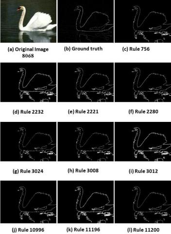
Through the visual inspection, there are many rules which provide the best results in term of edge continuity, thickness and accuracy. For image 8068, some of the best rules obtained are: 756, 2221, 2232, 2280, 2297, 2732, 3008, 3012, 3024, 10996, 10212, 11200, 11196. The correspondent edges are illustrated in Figure 4.
The OTCA rules can generate extremely thin lines (as Rule 3008, 11200) or extremely thick lines (as Rule 11196), depending on the rules used. While the remaining rules have varying degrees of thickness, they give a far better degree of continuity and smoothness.
Five rules are chosen in this paper: 672, 688, 736, 3008, and 3012, from the subset of best rules. Numerous alternative rules may work better for a particular sort of picture. However, in this study, we focus on those that consistently deliver the greatest outcomes over a wide variety of changes. It is critical to highlight that once the optimal rules are identified, they may be applied directly to an image, resulting in the desired output.
6.3 Visual results
This section discusses the outcomes of applying the extracted OTCA rules on a variety of images. They have demonstrated their efficiency in offering accurate edge detection. Experiments were conducted on a variety of different test images. Figure 4 illustrates some of the findings.
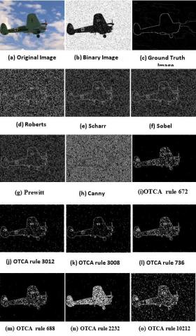
Figure 5 displays the identification of edges using several OTCA rules. The original images are represented by (a, d, g, and j). The ground truth pictures are (b, e, h, and k). (c, f, i and l) represent the results of applying OTCA rules, accordingly (3008,10212,688,736). The visual results indicate that the OTCA rules provide accurate and clean edges.
Figure 4. Results of various OTCA rules on image 8068
Figure 5. Application of various OTCA rules on images
Figure 6 displays the results of six selected OTCA rules, applied on image “48017.jpg”.
Figure 6. Results of selected rules on image “48017.jpg”
We observe that OTCA rules ensure that all edges are smooth and true. They provide fine, continuous borders. Additionally, depending on the rules set, the OTCA rules are capable of producing both very thin and clean lines. Moreover, OTCA rules provide more contrast than any other algorithm. The results are more appropriate for future investigation.
6.4 Numerical results
Image quality measurement is a crucial step in image processing applications. Indeed, the visual result is not sufficient to judge the quality of a contour. In the following, we use objective functions: RMSE and SSIM to evaluate the quality of the edges, extracted by OTCA rules.
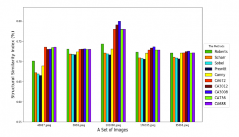
Table 3 shows a comparative study of various edge detection methods with SSIM function. The best values are highlighted in bold. The similar results are indicated in green, while red color signifies the worst result. Taken as an example image 8068, all the rules indicate the highest value among all of the other methods. The result of rules 672, 688 and 736 are similar to Roberts and better than Scharr, Sobel, Prewitt and Canny results. For all the tested images, we can conclude that the OTCA rules give very good results, better or equivalent to the standard edge detectors.
Table 3. Performance evaluation of different edge detection methods using SSIM
|
Images |
48017 |
8068 |
201080 |
176035 |
35008 |
|
Roberts |
0.71 |
0.73 |
0.743 |
0.723 |
0.721 |
|
Scharr |
0.672 |
0.718 |
0.721 |
0.709 |
0.711 |
|
Sobel |
0.669 |
0.718 |
0.719 |
0.708 |
0.709 |
|
Prewitt |
0.665 |
0.717 |
0.717 |
0.706 |
0.707 |
|
Canny |
0.689 |
0.724 |
0.731 |
0.726 |
0.721 |
|
CA672 |
0.736 |
0.73 |
0.78 |
0.729 |
0.722 |
|
CA3012 |
0.73 |
0.731 |
0.791 |
0.734 |
0.725 |
|
CA3008 |
0.731 |
0.732 |
0.8 |
0.737 |
0.725 |
|
CA736 |
0.735 |
0.73 |
0.779 |
0.728 |
0.721 |
|
CA688 |
0.736 |
0.73 |
0.78 |
0.729 |
0.722 |
Overall, we can perceive that the majority of the rules give the best results compared with the other methods. Taken as example image 48017, the rules 672 and 688 indicate the highest value among all of the other methods. In the case of image 35008, the result of rule 736 is similar to Roberts and Canny, and highest comparing with Scharr, Sobel and Prewitt. So on for all the tested images. The OTCA rules outperform classical edge detectors.
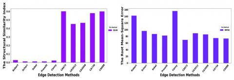
Figure 7 shows a graph comparison of SSIM values for the five images using OTCA rules and classical edge detectors.
Figure 7. Evaluation of edge detection methods with SSIM
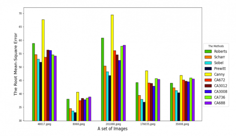
The comparison of edge detection methods utilizing the root mean square error (RMSE) is shown in Table 4. It is performed on five representative images. We can see that the RMSE vary between all the given methods. Some of the proposed rules have the best result, others are similar, and even there are some worst cases according to the recent method.
Table 4. Performance evaluation of different edge detection methods using RMSE
|
Images |
48017 |
8068 |
201080 |
176035 |
35008 |
|
Roberts |
58.8 |
37.98 |
60.79 |
44.23 |
44.00 |
|
Scharr |
54.64 |
34.5 |
50.38 |
39.41 |
42.29 |
|
Sobel |
52.95 |
33.62 |
48.21 |
37.9 |
41.21 |
|
Prewitt |
51.81 |
33.00 |
46.78 |
36.88 |
40.43 |
|
Canny |
67.65 |
40.63 |
69.49 |
48.6 |
46.88 |
|
CA672 |
53.68 |
37.58 |
56.10 |
44.08 |
45.13 |
|
CA3012 |
56.38 |
38.31 |
54.55 |
43.87 |
44.74 |
|
CA3008 |
56.20 |
37.8 |
52.45 |
42.88 |
44.5 |
|
CA736 |
54.53 |
38.4 |
57.78 |
45.73 |
45.92 |
|
CA688 |
54.08 |
38.84 |
58.11 |
45.39 |
45.51 |
Figure 8 shows a graph comparison of RMSE values for the five images using several methods.
Figure 8. Evaluation of several edge detection methods with RMSE
In the following, we have evaluated the execution time of OTCA rules and the most common algorithms in edge detection. The OTCA rules show superior improvement in terms of execution time.
Table 5. Execution time comparison between several methods
|
Images |
48017 |
8068 |
201080 |
176035 |
35008 |
|
Roberts |
0.0312 |
0.0156 |
0.0791 |
0.025 |
0.0310 |
|
Scharr |
0.0313 |
0.0312 |
0.0350 |
0.0313 |
0.0240 |
|
Sobel |
0.0313 |
0.0312 |
0.0250 |
0.0313 |
0.0240 |
|
Prewitt |
0.0312 |
0.0312 |
0.0270 |
0.0313 |
0.0330 |
|
Canny |
0.1249 |
0.1250 |
0.2884 |
0.111 |
0.1121 |
|
CA672 |
0.0157 |
0.0156 |
0.0160 |
0.0156 |
0.0150 |
|
CA3012 |
0.0156 |
0.0156 |
0.0160 |
0.0220 |
0.0290 |
|
CA3008 |
0.0156 |
0.0313 |
0.0180 |
0.0120 |
0.0150 |
|
CA736 |
0.0156 |
0.0156 |
0.0160 |
0.0156 |
0.0160 |
|
CA688 |
0.0156 |
0.0156 |
0.0150 |
0.0156 |
0.0150 |
Table 5 indicates the values of execution time for several edge detectors, and OTCA rules. Five images have been used to calculate the consuming edge detection time. The conclusion that emerges from the analysis of the data is:
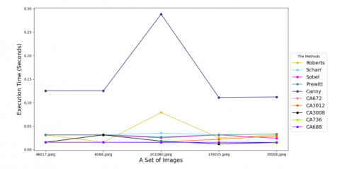
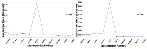
Figure 9 shows a graphical comparison of computational time between different edge detection methods using the five images.
Figure 9. Execution time of edge detection methods
It is clear that the execution times for OTCA rules are the lowest. They are represented by the lowest lines, all the values are below the limit of 0.032 s. The execution time values are reconciled for all rules. The blue line representing Canny, shows the worst results for all images (time greater than 0.11 s). We note that Canny and Roberts give the highest execution time for the image “201080.jpg”. The lines of Prewitt, Scharr and Sobel are very close.
A robust solution that is adjustable to the different noise levels in images requires an effective edge detection method. Additionally, it facilitates in the differentiation of real picture contents from visual artifacts generated by noise.
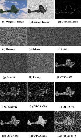
Traditionally used edge detectors frequently fail to handle images with a poor object outline or a high level of noise [43]. The purpose of this section is to evaluate the efficacy of OTCA rules on noisy images. To the original picture, a salt and pepper noise is applied. We use OTCA rules and compare them to traditional edge detectors.
7.1 Under salt and pepper 10%
Figure 10. Experiments on noisy image with different edge detectors (salt and pepper 10%)
Figure 10 presents experiments on a noisy image with different edge detection methods under 10% Salt and Pepper noise. It clearly shows the effectiveness of OTCA rules to perform edge detection even on noisy images. The results show a small variation due to the noise edges. The edges of Roberts, Sobel, Scharr, and Prewitt are less continuous comparing with Canny and the OTCA rules due to the noise pixels present in the resulting image.
Table 6 indicates the evaluation of several edge detection methods using SSIM and RMSE with run time computation under 10% Salt and Pepper noise, on Plane image.
Table 6. Evaluation of several edge detection methods on a noisy image with 10% salt and pepper noise
|
Methods |
SSIM |
RMSE |
Time |
|
Roberts |
0.15337731 |
108.072859 |
0.03802776 |
|
Scharr |
0.08764633 |
73.897366 |
0.02601743 |
|
Sobel |
0.08401032 |
67.1350391 |
0.03902721 |
|
Prewitt |
0.07936585 |
63.791198 |
0.03203011 |
|
Canny |
0.07020513 |
149.751714 |
0.30710697 |
|
CA672 |
0.67409452 |
49.2556559 |
0.01503539 |
|
CA3012 |
0.67024881 |
48.0975436 |
0.01601172 |
|
CA3008 |
0.68371942 |
44.4847335 |
0.02001452 |
|
CA736 |
0.67194186 |
50.588171 |
0.01504016 |
|
CA688 |
0.67388888 |
50.8091482 |
0.02802038 |
The OTCA rules achieve the best results in comparison with other classical edge detectors. For SSIM fitness, the best values are obtained for the OTCA rules, the minimum is 0.67, while for conventional methods, it does not exceed 0.15 (Roberts). For RMSE fitness, the minimum values, so the best were achieved by the OTCA rules, the best is 44.48. the minimum value achieved by conventional detectors is 63.79, while the worst fitness goes up to 149.75 (Canny). The numerical evaluation reinforces the visual inspection made in Figure 10.
Figure 11 illustrates a graph comparison of SSIM and RMSE for the edge detection methods with 10% of noise.
This graph clearly shows the superiority of OTCA rules over conventional detectors. The SSIM values for OTCA rules significantly exceed those obtained for traditional methods.
Figure 11. SSIM and RMSE evaluation for a noisy image under 10% Salt and Pepper noise
7.2 Under salt and pepper 20%
By increasing the noise level to 20% (Figure 12), the results indicate a quick decline in the quality value for each of the approaches presented. Roberts, Sobel, Scharr, and Prewitt produced discontinuous edges and obliterated the object's borders with noise. The image is covered with short false edge lines as a result of the Canny edge detector's results. OTCA rules have a reasonably high level of resistance to increased noise levels. Although the picture has the potential to attenuate areas with cumulated noise, it begins to introduce discontinuities in the edges.
Figure 12. Experiments on noisy image with different edge detection method (20% Salt and Pepper)
Table 7 mentions the evaluation of several edge detection methods using SSIM and RMSE with run time computation under 20% Salt and Pepper noise.
Table 7. Evaluation of several edge detection methods on a noisy image with 20% of salt and pepper noise
|
Methods |
SSIM |
RMSE |
Time |
|
Robert |
0.02748159 |
142.048855 |
0.02601981 |
|
Scharr |
0.01183269 |
96.1329276 |
0.02602005 |
|
Sobel |
0.01274323 |
86.9824602 |
0.03602552 |
|
Prewitt |
0.01246828 |
82.4232013 |
0.03104734 |
|
Canny |
0.0229231 |
155.899538 |
0.21615362 |
|
CA672 |
0.60168757 |
69.5031391 |
0.01500821 |
|
CA3012 |
0.45255388 |
89.1974676 |
0.01500988 |
|
CA3008 |
0.46481212 |
85.8998185 |
0.01604176 |
|
CA736 |
0.57875446 |
74.6796182 |
0.01600671 |
|
CA688 |
0.60022728 |
73.526359 |
0.01604176 |
We can extract from the data that OTCA rules takes a large benefit over the classical methods. It gained the best SSIM and RMSE with less consuming time. For SSIM fitness, the highest value is provided by rule 672 (0.601). The best score for RMSE was achieved by rule 688 (73.52). Regarding execution time, we note that the best times are recorded for OTCA rules (of the order of 0.01), while conventional detectors record higher times.
The results reveal that the quality value of all approaches is rapidly decreasing. Nevertheless, OTCA rules retain their advantage over the classical edge detectors. They produce the highest quality value with noise comparing to the other methods besides the less consuming time. Figure 13 illustrates a graph comparison of the methods with 20% of noise.
Figure 14 illustrates a run time graph comparison of different methods.
It can be seen, that for both cases of 10% and 20% noise, the runtime obtained for all OTCA rules is better than those of the classic methods, noting that the highest peak was achieved by Canny detector.
Figure 13. Fitness values for different edge detection methods under 20% Salt and Pepper noise
Figure 14. A run time graph comparison for different edge detection methods under 10%, 20% Salt and Pepper noise respectively
In this article, we have provided a novel and efficient approach for edge detection. It is based on an Outer Totalistic Cellular Automata. The best transition rules are extracted and provided very satisfactory results. The proposed approach is validated and tested on images from Berkeley dataset. Comparison is made with classical edge detectors like Canny, Sobel, Prewitt… etc. Numerical performance is provided by fitness functions: RMSE and SSIM. Execution time is also compared. Cellular Automata have been found to be efficient for image processing, as edge detection is one of the most difficult image processing problems. OTCA rules provide best accuracy while ensuring a lowest execution time.
Additional experience dealing with noisy images, showed that the OTCA rules perform better than classical edge detectors, it is striking to note, that where other edge detectors fail, a simple rule of our OTCA provide very good results, in terms of edge quality and time execution.
OTCA rules were shown to be extremely competitive, robust, and outperformed classical algorithms.
The outcomes are promising. It is feasible to derive some effective rules for performing complex image processing tasks like edge detection. The obtained rule sets are extremely simple as they contain only a single rule with the performance and efficiency up to the mark. The result of the learned rules has also been compared with some standard edge detectors, and it has been found that in most cases its performance is better than the standard edge detectors. Specifically, in the run time process, the rules give an effective faster time. Besides that, the OTCA rules have a large advantage when they deal with noised images. This attests the robustness of our OTCA.
Future work can focus on the study of other kinds of cellular automata for different image enhancement tasks, and finding more efficient methods to deal with the problem of optimizing the large set of transition rules.
Furthermore, some advanced concepts related to CA can be inculcated to improve the performance and it is conceivable to modify the CA rules in order to address additional challenges. The Deep Learning concepts should be explored for optimization of rules.
[1] Zhai, L., Dong, S., Ma, H. (2008). Recent methods and applications on image edge detection. In 2008 International Workshop on Education Technology and Training & 2008 International Workshop on Geoscience and Remote Sensing, 1: 332-335. http://dx.doi.org/10.1109/ETTandGRS.2008.39
[2] Vincent, O.R., Folorunso, O. (2009). A descriptive algorithm for Sobel image edge detection. In Proceedings of Informing Science & It Education Conference (InSITE), 9: 97-107. http://dx.doi.org/10.28945/3351
[3] Mohammed, J., Nayak, D.R. (2014). An efficient edge detection technique by two dimensional rectangular cellular automata. In International Conference on Information Communication and Embedded Systems (ICICES2014), pp. 1-4. http://dx.doi.org/10.1109/ICICES.2014.7033847
[4] Zhai, L., Dong, S., Ma, H. (2008). Recent methods and applications on image edge detection. In 2008 International Workshop on Education Technology and Training & 2008 International Workshop on Geoscience and Remote Sensing, pp. 332-335. http://dx.doi.org/10.1109/ETTandGRS.2008.39
[5] Canny, J. (1986). A computational approach to edge detection. IEEE Transactions on Pattern Analysis and Machine Intelligence, 8(6): 679-698. http://dx.doi.org/10.1109/TPAMI.1986.4767851
[6] Deriche, R. (1990). Fast algorithms for low-level vision. IEEE Transactions on Pattern Analysis and Machine Intelligence, 12(1): 78-87. http://dx.doi.org/10.1109/34.41386
[7] Hildreth, E., Marr, D. (1980). Theory of edge detection. Proceedings of Royal Society of London, 207(1167): 187-217. https://doi.org/10.1098/rspb.1980.0020
[8] Marr D. (1982). Vision. W. H. Freeman and Company, San Fransisco.
[9] Wolfram, S. (2002). A new kind of science. Appl. Mech. Rev., 56(2): B18-B19. http://dx.doi.org/10.1115/1.1553433
[10] Nayak, D.R., Patra, P.K., Mahapatra, A. (2014). A survey on two dimensional cellular automata and its application in image processing. arXiv preprint arXiv:1407.7626.
[11] Goles, E., Martínez, S. (2013). Cellular automata and complex systems (Vol. 3). Springer Science & Business Media. http://dx.doi.org/10.1007/978-94-015-9223-9
[12] Ortigoza, G.M. (2015). Implementation of three-dimensional cellular automata on irregular geometries: Medical simulations on surfaces and volumes. In Mathematics and Its Applications, Chapter 3, pp. 75-99. https://www.fcfm.buap.mx/cima/public/docs/publicaciones/MatematicasYSusAplicaciones5.pdf.
[13] Sarkar, P. (2000). A brief history of cellular automata. ACM Computing Surveys (CSUR), 32(1): 80-107. http://dx.doi.org/10.1145/349194.349202
[14] Rosin, P.L. (2005). Training cellular automata for image processing. In Scandinavian Conference on Image Analysis, Springer, Berlin, Heidelberg, pp. 195-204. http://dx.doi.org/10.1007/11499145_22
[15] Rosin, P.L. (2010). Image processing using 3-state cellular automata. Computer vision and image understanding, 114(7): 790-802. http://dx.doi.org/10.1016/j.cviu.2010.02.005
[16] Preston Jr, K., Duff, M.J. (2013). Modern cellular automata: Theory and applications. Springer Science & Business Media. http://dx.doi.org/10.1007/978-1-4899-0393-8
[17] Diosan, L. , Andreica, A., Enescu, A. (2017). The use of simple cellular automata in image processing. Studia Universitatis Babes,-Bolyai Informatica, 62(1): 5-14. http://doi.org/10.24193/subbi.2017.1.01
[18] Wongthanavasu, S., Sadananda, R. (2003). A CA-based edge operator and its performance evaluation. Journal of Visual Communication and Image Representation, 14(2): 83-96. http://dx.doi.org/10.1016/S1047-3203(03)00022-1
[19] Chang, C.L., Zhang, Y.J., Gdong, Y.Y. (2004). Cellular automata for edge detection of images. In Proceedings of 2004 International Conference on Machine Learning and Cybernetics (IEEE Cat. No. 04EX826), 6: 3830-3834. IEEE. http://dx.doi.org/10.1109/ICMLC.2004.1380502
[20] Ha, Y. (2008). Method of edge detection based on Non-linear cellular Automata. In 2008 7th World Congress on Intelligent Control and Automation, pp. 6817-6821. http://dx.doi.org/10.1109/WCICA.2008.4593966
[21] Ke, Z., Weihua, Z., Jinsha, Y. (2008). Edge detection of images based on cloud model cellular automata. In 2008 27th Chinese Control Conference, pp. 249-253. http://dx.doi.org/10.1109/CHICC.2008.4604887
[22] Liu, S., Wan, Q., Zhang, H. (2009). Edge detection of fabric defect based on fuzzy cellular automata. In 2009 International Workshop on Intelligent Systems and Applications, pp. 1-3. http://dx.doi.org/10.1109/IWISA.2009.5072841
[23] Kumar, T., Sahoo, G. (2010). A novel method of edge detection using cellular automata. International Journal of Computer Applications, 9(4): 38-44. http://dx.doi.org/10.5120/1371-1848
[24] Djemame, S., Batouche, M. (2012). Combining cellular automata and particle swarm optimization for edge detection. International Journal of Computer Applications, 57(14): 16-22. http://doi.org/10.13140/RG.2.1.3284.9443
[25] Zagoris, K., Pratikakis, I. (2012). Scene text detection on images using cellular automata. In International Conference on Cellular Automata, pp. 514-523. http://dx.doi.org/10.1007/978-3-642-33350-7_53
[26] Dhillon, P.K. (2012). A novel framework to image edge detection using cellular automata. Int. J. Comput. Appl, 1: 1-5.
[27] Priego, B., Bellas, F., Souto, D., López-Peña, F., Duro, R.J. (2012). Evolving cellular automata for detecting edges in hyperspectral images. In 2012 IEEE International Conference on Fuzzy Systems, pp. 1-6. http://dx.doi.org/10.1109/FUZZ-IEEE.2012.6251156
[28] Gorsevski, P.V., Onasch, C.M., Farver, J.R., Ye, X. (2012). Detecting grain boundaries in deformed rocks using a cellular automata approach. Computers & Geosciences, 42: 136-142. http://dx.doi.org/10.1016/j.cageo.2011.09.008
[29] Uguz, S., Sahin, U., Sahin, F. (2013). Uniform cellular automata linear rules for edge detection. In 2013 IEEE International Conference on Systems, Man, and Cybernetics, pp. 2945-2950. http://dx.doi.org/10.1109/SMC.2013.502
[30] Sahin, U., Sahin, F., Uguz, S. (2013). Hybridized fuzzy cellular automata thresholding algorithm for edge detection optimized by PSO. In 2013 High Capacity Optical Networks and Emerging/Enabling Technologies, pp. 228-232. http://dx.doi.org/10.1109/HONET.2013.6729792
[31] Diwakar, M., Patel, P.K., Gupta, K. (2013). Cellular automata based edge-detection for brain tumor. In 2013 International Conference on Advances in Computing, Communications and Informatics (ICACCI), pp. 53-59. http://dx.doi.org/10.1109/ICACCI.2013.6637146
[32] Rosin, P.L., Sun, X. (2014). Edge detection using cellular automata. In Cellular Automata in Image Processing and Geometry. Springer, Cham, 10: 85-103. http://dx.doi.org/10.1007/978-3-319-06431-4_5
[33] Mofrad, M.H., Sadeghi, S., Rezvanian, A., Meybodi, M.R. (2015). Cellular edge detection: Combining cellular automata and cellular learning automata. AEU-International Journal of Electronics and Communications, 69(9): 1282-1290. https://doi.org/10.1016/j.aeue.2015.05.010
[34] Han, M., Yang, X., Jiang, E. (2016). An extreme learning machine based on cellular automata of edge detection for remote sensing images. Neurocomputing, 198: 27-34. http://dx.doi.org/10.1016/j.neucom.2015.08.121
[35] Amrogowicz, S., Zhao, Y.T., Zhao, Y.F. (2016). An edge detection method using outer Totalistic Cellular Automata. Neurocomputing, 214: 643-653. http://dx.doi.org/10.1016/j.neucom.2016.05.092
[36] Aghaei, A. (2018). A cellular Automata approach for noisy images edge detection under null boundary conditions. In 2018 Second International Conference on Computing Methodologies and Communication (ICCMC), pp. 771-777. http://dx.doi.org/10.1109/ICCMC.2018.8487526
[37] Enescu, A., Andreica, A., Dioşan, L. (2019). Evolved Cellular Automata for Edge Detection in Binary Images. In 2019 IEEE 15th International Conference on Intelligent Computer Communication and Processing (ICCP), pp. 351-358. http://dx.doi.org/10.1109/ICCP48234.2019.8959658
[38] Kazar, O., Slatnia, S. (2011). Evolutionary cellular automata for image segmentation and noise filtering using genetic algorithms. Journal of Applied Computer Science and Mathematics, 5(10): 33-40.
[39] Djemame, S., Batouche, M., Oulhadj, H., Siarry, P. (2019). Solving reverse emergence with quantum PSO application to image processing. Soft Computing, 23(16): 6921-6935. http://dx.doi.org/10.1007/s00500-018-3331-6
[40] Djemame, S., Batouche, M. (2018). A hybrid metaheuristic algorithm based on quantum genetic computing for image segmentation. In Hybrid Metaheuristics for Image Analysis, pp. 33-48. http://dx.doi.org/10.1007/978-3-319-77625-5_2
[41] Phillips, J.B., Eliasson, H. (2018). Camera Image Quality Benchmarking. John Wiley & Sons. http://dx.doi.org/10.1002/9781119054504
[42] https://www2.eecs.berkeley.edu/Research/Projects/CS/vision/grouping/resources.html, accessed on May 4th, 2021.
[43] Breukelaar, R., Bäck, T. (2004). Evolving transition rules for multi dimensional cellular automata. In International Conference on Cellular Automata, pp. 182-191. http://dx.doi.org/10.1007/978-3-540-30479-1_19