Malathi Devendran | Indumathi Rajendran | Vijayakumar Ponnusamy* | Diwakar R. Marur
© 2021 IIETA. This article is published by IIETA and is licensed under the CC BY 4.0 license (http://creativecommons.org/licenses/by/4.0/).
OPEN ACCESS
In recent years, machine learning algorithms related to images have been widely utilized by Convolution Neural Networks (CNN), and it has a high accuracy for recognition of an image. As CNN contains large number of computations, hardware accelerator like Field Programmable Gate Array is employed. Quite 90 % of operations during a CNN involves convolution. The objective of this work is to scale back the computation time to increase the peak, width and the pixel intensity levels in the input image. The execution time of a image processing program is mostly spent on loops. Loop optimization is a process of accelerating speed and reducing the overheads related to loops. It plays a crucial role in improving performance and making effective use of multiprocessing capabilities. Loop unrolling is one of the loop optimization techniques. In our work CNN with four levels of loop unrolling is used. Due to this delay is reduced compared with conventional Xilinix. With the assistance of strides and padding the 40 % of computation time has been reduced and is verified in MATLAB.
Convolutional Neural Networks (CNN), delay, loop unrolling, padding, stride
CNN contains a huge number of computations, so it is required to accelerate these CNN computations by a hardware accelerator, like Field Programmable Gate Array (FPGA), Graphics Processing Unit (GPU), and Application Specific Integrated Circuit (ASIC) designs. Although, these CNN accelerator faces a difficult problem because it has the huge computation time and consumption of power is occurred by the memory for information access.
In CNN, it has almost exclusively been associated with computer vision applications because their architecture is specifically fitted to performing complex visual analyses. Instead, the standard two-dimensional array in CNN architecture has the three-dimensional arrangement of neurons [1].
The convolutional layer is that the first layer of CNN. In the CNN layer, it has the neurons in each neuron it only processes the information from a small part of the visual field. Rectified Layer Unit (ReLU) is the second layer of CNN which is followed by the convolutional layer. In ReLU layer enables the CNN to handle complicated information. The third layer is that the fully connected layer, where the entire inputs are to be connected to the upcoming layer shown in Figure 1. CNN is mainly used in machine vision and self-driving vehicles for object recognition applications.
1.1 Convolution layer Rectified layer unit
The convolution operation in the CNN extracts the features from the input. In the convolutional layer, it has two levels of features such as low-level and high-level. In CNN layers extract the edges, lines and corners are named as low-level layers feature. Higher levels of features are extracted using higher levels of layers [2]. The input has the size of N × N × D and the kernel has the size of K × K × D. The output is produced with the help of convolution of input with the kernel. Each kernel is moved from left to right based on the strides from the top left corner to the bottom right corner.
Figure 1. Layers in CNN
1.2 Pooling and subsampling layer
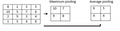
Figure 2. Representation of pooling
To reduce the resolution of the feature maps in the CNN, an additional layer is used. Because it makes the features robust against noise and distortion of the image. Maximum and average pooling, two levels were used. In maximum pooling, the maximum number of values has been taken from the matrix [3, 4]. In average pooling, the average value has been taken from the input feature image. Here input size is 4x4 and the subsampling is 2x2 so the input size is divided into four 2x2 matrixes and there is no overlapping matrix shown in Figure 2.
1.3 Rectified layer unit
In ReLU it has the size of the input and output layers are the same because it implements the function y = max (x, 0). It uses nonlinear properties so the performance was increased for the overall network without affecting the other convolutional layers. The advantage of ReLU is the network trains many times faster than another network [5]. In ReLU it has the activation function in a linear manner either a positive value or zero there is no negative value. If there is any negative value is present that value will become zero is shown in Figure 3.
Figure 3. Representation of ReLU functionality
1.4 Fully connected layers
The fully connected layer is the final layer of the CNN. The most important component for recognizing and classifying the image for computer vision application is done by a fully connected layer. The process of CNN starts with convolution and pooling layer and partitioning the image into features. Finally, the result is given to the fully connected layer for the final classification decision. The entire inputs are connected to upcoming layers of the CNN [6].
2.1 Loop rolling
In the loop optimizing technique, loop rolling was used to perform the convolution operation. Loop optimizing technique is most important to perform operations in the neural network. Under the loop optimizing technique loop rolling and loop unrolling are used. In the loop rolling method, it gives the larger design space so it affects the processing engine architecture with the help of memory and data reuse. In convolution networks, it has four levels of loops [7] So, different levels of nested convolution loops lead to different types of parallelization of computations. For example, three levels nested can result in three parallel computing. The limitation of loop rolling is it has a high computation time to perform any operations in different levels of loops. Loop unrolling is used to reduce the computation time.
2.2 Stride
Stride could be an element of CNNs or Neural Networks tuned for the compression of pictures and video information. Stride represents the number of pixels skipping in the convolution operation. more the strip size, less the computational complexity but lesser the accuracy. The Stride size can be selected optimally without compromising the accuracy and computational complexity. on other hand, it determines the feature size (which determine the accuracy and computational complexity) which will be generated in the convolution operation i.e.
Feature size=((image size-kernel size)/ Stride)+1
Stride could be a parameter of the neural network filter that modifies the number of movements over the image or video [8]. As an example, if a neural network stride is ready to one, the filter can move one constituent unit, at a time. The Scale affects the encoded output volume, therefore stride is commonly set to an entire whole number, instead of a fraction or decimal.
To calculate the output matrix the Eq. (1) is used. Where N is the input matrix dimension and F is the feature map dimension or another input matrix dimension, P is the padding if padding is added in the given input matrix it becomes 1 otherwise it will be 0 and S is the stride:
$O=\frac{N-F+2 P}{S}+1$ (1)
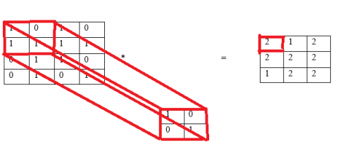
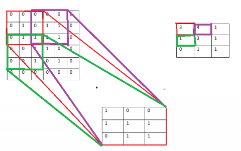
Stride (S) is that the range of pixels that move over the column and row pixels in input. Once the value S is one then it tends to shifts the one pixel in a column or row. Once the is two then it tends to shift the two pixels. Figure 4 shows the calculation of the output matrix. In this figure, N is 4 and F is 2 and there is no padding is applied so P is 0, and stride S is 1. From Eq. (1) the output matrix will be 3. The calculation of output value in the first cell is $(1 \times 1)+(0 \times 0)+(1 \times 0)+(1 \times 1)=1+0+0+1=2$.
Figure 4. Output matrix cell 1 using S = 1
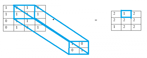
Figure 5 shows the output calculation in second cell using stride. The calculation of output value in the second cell is $(0 \times 1)+(1 \times 0)+(1 \times 0)+(1 \times $$1)=0+0+0+1=1$. After applying the stride is 1 in the column, the dimensions become 3.
Figure 5. Output matrix cell 2 using S = 1
The calculation of output value in the first cell in second row is $(1 \times 1)+(1 \times 0)+(0 \times 0)+(1 \times 1)=1+0+0+1=2$. The limitation is correct level at the output cannot be achieved. From the example 3x3 output matrix is used instead of 4x4 because in the input matrix 4x4 some loss of information is occurred. The purpose of convolution operation is to carry out edge enhancement. When a 3x3 matrix is used as a kernel, then the loss of information is very limited compared to the use of a 4x4 kernel for edge enhancement.
3.1 Accelerator
It involves the outsized quantity of knowledge and weights. The memory is poor for saving information because it required Gigabytes of memory is needed to store the data. Three levels of storage hierarchy: 1) memory; 2) buffers; 3) registers which are illustrated in Figure 6. The design method is to take the informed memory and it is transferred to the buffer. The output of buffers is given to array blocks to perform convolution [9, 10]. Once the process is completed the result is transferred to buffers and it will be transferred to memory which is used to input as upcoming layers.
Figure 6. CNN accelerator hierarchy
3.2 Levels of convolution loops
Figure 7. Four levels of convolution loops
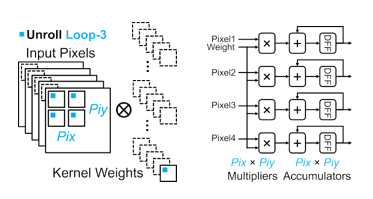
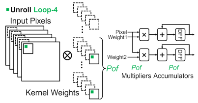
In CNN algorithms convolution is the important operation that performs multiply and accumulates for input along with kernel weights. The pseudocodes for the four-level of convolutions as shown in Figure 7. There are three loop optimizing techniques were used to perform convolution in an efficient manner [11]. Loop unrolling, loop tilling, and loop interchange. In the hardware accelerator FPGA implementation, the three-loop optimizing techniques will not increase the computational overhead because, those mechanisms are converted into a logic block of the circuit which will respond immediately once powered up. Loop unrolling is one of the loop optimization techniques used to optimize the program execution speed and perform parallel computation. It reduces the loop overhead and increases the program efficiency. Loop tilling is to divide the entire input data into a small level of multiple levels of blocks so it can be easily stored in buffers. Loop interchange which finds an order of computations of four levels of loops. In the loop, the interchange has the intratile loop which is used to find the order of data movements from buffers to registers. In the intertile loop find the order of computation from external memory to buffers [12]. There are four levels of loop unrolling involved in CNN.
Loop 1 unrolling the convolution is performed for pixels and weights are totally from the different location but within the same input matrix and another input, matrix computed every time. The adder tree is required to add the previous partial sum outputs shown in Figure 8. Loop 2 unrolling the convolution is performed for pixels and weights are from the equal location but different same input matrix and another input matrix computed in every time shown in Figure 9 [13, 14]. In loop unrolling 3 the pixels are from the different location in the corresponding input matrix is multiplies with the unit weight. Here no adder tree is required to reuse the pixels and for parallel computations shown in Figure 10. In loop unrolling 4 the identical pixel is multiplied with the pixels in the same location but different features shown in Figure 11 [15, 16].
Figure 8. Loop 1 for unrolling
Figure 9. Loop 2 for unrolling
Figure 10. Loop 3 for unrolling
Figure 11. Loop 4 for unrolling
3.3 Strides and padding
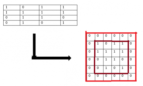
Stride (S) is that the range of pixels that move over the column and row pixels in input. Once the S value is one then it tends to shifts the one pixel in a column or row. Once the S is two then it tends to shift the two pixels. Padding may be a term relevant to CNN because it refers to the number of pixels added to a picture once it’s being processed by the kernel of a CNN. The zero value is to be added in the row and column of the input image if the padding is zero. In normal convolution.
Figure 12. Output matrix after applying padding
The overlap occurs in the middle of stages and the corner of the input image is used less to perform the convolution along with the kernel. To reduce the overlap and make efficient use of edges padding, stride 2 were used. Figure 12 shows the output matrix after applying zero padding. Here the normal input matrix dimension is 4x4 after applying the padding the dimension has changed to 6*6 matrix. From the figure zero's are added in row and column to get the accurate dimensions. The brown box is the normal input matrix and the red color box is the after adding padding.
3.3.1 Calculation for stride is 1 and 2 without padding (S = 1, S = 2 and P = 0)
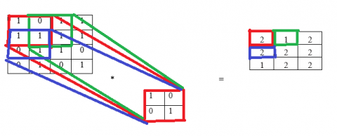
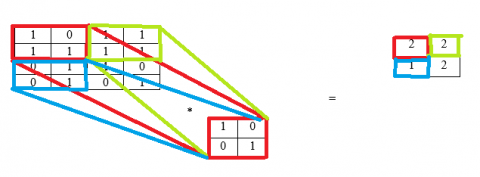
Figure 13 shows the output matrix calculation using S = 1 and P = 0, N = 4, F = 2. The calculation of output value in the first cell is $(1 \times 1)+(1 \times 0)+(0 \times 0)+(1 \times 1)=1+0+$$0+1=2$. The calculation of output value in the second cell is $(1 \times 1)+(1 \times 0)+(1 \times 0)+(1 \times 1)=1+0+0+$$1=2$. Here the stride is 1 the column of the input matrix is shifted by one. The red color 2x2 matrix is taken first and multiplies with another 2x2 feature matrix and the output is displayed in the first cell of the output matrix (red color box). The green color box indicates the after shifting one column and then multiplied with another matrix and the result will be displayed in the output matrix (green color box). The limitation is e cannot get the correct level at the output. From the example, a 3x3 output matrix is obtained instead of getting 4x4 because the input matrix is 4x4 so some loss of information has occurred. Figure 14 shows the output matrix calculation using S = 2 and P = 0, N = 4, F = 2. Here stride is 2 the column of the input matrix is shifted by two. The red color 2x2 matrix is taken first and multiply with another 2x2 feature matrix and the output is displayed in the first cell of the output matrix (red color box). The light green color box indicates the after shifting one column and then multiplied with another matrix and the result will be displayed in the output matrix (light green color box).
Figure 13. Output matrix S = 1 and P = 0
Figure 14. Output matrix S = 2 and P = 0
Figure 15 shows the output matrix calculation using S = 1 and P = 1, N = 4, F = 2 so output is 4. The calculation of output value in the first cell is (0*1) + (0*0) + (0*0) + (0*1) + (1*1) + (0*1) + (0*0) + (1*1) + (1*1) = 0 + 0 + 0 + 0 + 1 + 0 + 0 +0 + 1 + 1 = 3. Here stride is 1 the column of input matrix is shifted by one. The red colour 3*3 matrix is taken first and multiply with another 3*3 feature matrix and the output is displayed in first cell of the output matrix (red colour box). The green colour box indicates the after shifting one column and then multiplied with another matrix and result will displayed in output matrix (green colour box). Here the input matrix is 4*4 and it becomes 6*6 after applying padding, so 4*4 output matrix is obtained.
Figure 15. Output matrix S = 1 and P = 1
When stride is 2, the column of the input matrix is shifted by one. The red color 3*3 matrix is taken first and multiplies with another 3*3 feature matrix and the output is displayed in the first cell of the output matrix (red color box). The green color box indicates the after shifting one column and then multiplied with another matrix and the result will be displayed in the output matrix (green color box). Here the input matrix is 4*4 and it becomes 6*6 after applying padding, so a 3*3 output matrix is obtained as shown in Figure 16.
Figure 16. Output matrix S = 2 and P = 1
Loop 1 unrolling convolution is performed for pixels and weights are totally from the different location but within the same input matrix and another input and the matrix is computed every time. There are four adders and four multipliers are needed to perform MAC operation. In loop 2 unrolling the convolution is performed for pixels and weights are from the equal location but different same input matrix and another input matrix computed in every time. There are four adders and four multipliers are needed to perform MAC operation. In loop unrolling 3 the pixels are from the different location in the corresponding input matrix is multiplied with the unit weight. Here no adder tree is required to reuse the pixels and for parallel computations. In loop unrolling 4 the identical pixel is multiplied with the pixels in the same location but different features.
For stride 1 and without padding, the input matrix is 4x4 and the feature matrix is 2x2 so the output matrix becomes 3x3. Here parallel multiplication is performed with the help of loop unrolling. From the output matrix, a 3x3 matrix is obtained instead of getting 4x4. For stride is 2 the output matrix becomes 2x2. For stride 1 and with padding, the input matrix is 4*4 and the feature matrix is 2*2. After zero padding is added in the input matrix it becomes 6*6 matrix so the output matrix becomes 4*4. Here parallel multiplication is performed with same input matrix and another input and the matrix with the help of loop unrolling. From the output matrix, a 4*4 matrix is obtained from the input 4*4 matrix. If stride is 2 means the output matrix will be 3*3.
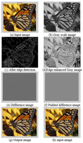
Edge enhancement mechanism is taken for testing and giving visual illustration for the proposed method of loop unrolled convolution operation using MATLAB Tool. Figure 17 (a) is the input image is converted into a greyscale image and then by using the edge detection algorithm edges are detected and then pixels are extracted from the given edge detection image. Figure 17 (b) to (f) provides the outcome various image operations on input image. By using the stride as 2 and padding the blocks are detected. The output image with the size of 256 x 256 is shown in Figure 17 (g) and the input image shown in Figure 17 (h) is of size 256 x 256. The output image has a higher pixel intensity level with respect to the input image, due to edge enhancement operation carried out on input image.
Figure 17. (a - f) Input image under various image processing operations and (h and g) for input and output comparison
4.1 Comparison of time and performance using MATLAB
The computation time loop rolling and loop unrolling is discussed. For the given application, loop rolling takes 239.51 seconds to operate. In loop unrolling it takes 81.86 seconds. Thus, loop unrolling takes less time compared with the loop rolling method. This in turn reduced the power by 40 % with the help of the loop unrolling method. There are several ways to measure power reduction due to the loop unrolling method. The Xilinx power estimator tool is used to extract the power consumption in Convolution operation without unrolling and with unrolling. These results are compared the 40% reduction is computed.
Table 1 shows the input and output data analysis in terms of standard deviation and pixel intensity. From the input and output, the height and width get increased so deviation has changed in output data deviation. There is no change in pixel image data. In the entropy, output images have a high entropy level that means pixel intensity values are high and it has a low standard deviation.
Table 1. Performance analysis of unrolling
|
Parameter |
Input Image |
Output Image |
|
Deviation |
0.3760 |
0.3778 |
|
Max. Pixel Image Data |
0.6265 |
0.6265 |
|
Entropy |
7.785 |
7.7329 |
|
Standard Deviation |
0.2789 |
0.2632 |
4.2 Comparison of delay using XILINX
Stride 1 has the 18.025 ns delay for computing the convolution operation using stride is 1 and with zero padding for input image size 256x256. For stride is 2 with zero padding has the 18.008 ns delay for computing the convolution operation using stride is 2 and with zero padding. From the comparison of delay stride is 2 has the lowest delay compared with stride is 1. Delay has been reduced from 18.025 ns to 18.008 ns.
In the loop optimization process, loop unrolling is used to optimize the program execution speed. It also increases the program efficiency. The execution time of a scientific program is mostly spent on loops to scale back the loop overhead and computation time loop unrolling was used. There are four levels of loop unrolling technique and it reduces the loop overhead in the loop optimizing technique. In loop unrolling it can be executed in a parallel manner. By employing loop unrolling, delay is reduced from 18.025 ns to 18.008 ns. The computation time is reduced by 40 % compared with loop rolling. Output image has a low standard deviation and high pixel intensity for the image. This work can be extended to analyze performance of loop unrolling techniques in FPGA based on delay and time required for training a CNN using different stride values and padding.
[1] Ma, Y.F., Cao, S., Vrudhula, S., Seo, J. (2018). Optimizing the convolution operation to accelerate deep neural networks on FPGA. IEEE Transactions on Very Large Scale Integration (VLSI) Systems, 26: 1354-1367. https://doi.org/10.1109/TVLSI.2018.2815603
[2] Bosi, B., Bois, G., Savaria, Y. (2017). Reconfigurable pipelined 2-D convolvers for fast digital signal processing. IEEE Transaction of Very Large Scale Integration (VLSI) Syst., 7(3): 299-308. https://doi.org/10.1109/92.784091
[3] Chen, Y., Krishna, T., Emer, J.S., Sze, V. (2017). Eyeriss: An energy-efficient reconfigurable accelerator for deep convolutional neural networks. IEEE Journal of Solid-State Circuits, 51(1): 127-138. https://doi.org/10.1109/JSSC.2016.2616357
[4] Zhang, C., Li, P., Sun, G.Y., et al. (2015). Optimizing FPGA-based accelerator design for deep convolutional neural networks, ACM/SIGDA International Symposium of Field Program Gate Arrays (FPGA), pp. 161-170. https://doi.org/10.1145/2684746.2689060
[5] Desoli, G., Chawla, N., Boesch, T., et al. (2017). A 2.9 TOPS/W deep convolutional neural network SoC in FD-SOI 28nm for intelligent embedded systems. In Solid-State Circuits Conference, pp. 14-34.
[6] Guan, Y.J., Liang, H., Xu, N.Y. et al. (2017). FP-DNN: An automated framework for mapping deep neural networks onto FPGAs with RTL-HLS hybrid templates. 2017 IEEE 25th Annual International Symposium on Field-Programmable Custom Computing Machines (FCCM), pp. 152-159. https://doi.org/10.1109/FCCM.2017.25
[7] Chen. Y.H., Emer, J.S., Sze, V. (2016). Eyeriss: A spatial architecture for energy-efficient dataflow for convolutional neural networks. ACM/IEEE International Symposium of Computer Architecture (ISCA), pp. 367-379. https://doi.org/10.1109/ISCA.2016.40
[8] Li, H.M., Fan, X.T., Jiao, L., Cao, W., Zhou, X.G., Wang, L.L. (2016). A high performance FPGA-based accelerator for large scale convolutional neural networks. IEEE International Conference of Field-Program. Logic Application (FPL), pp. 1-9. https://doi.org/10.1109/FPL.2016.7577308
[9] Ma, Y.F., Cao, Y., Vrudhula, S., Seo, J. (2017). Optimizing loop operation and dataflow in FPGA acceleration of deep convolutional neural networks. ACM/SIGDA International Journal of Field-Program. Gate Arrays (FPGA), pp. 45-54. https://doi.org/10.1145/3020078.3021736
[10] Ma, Y.F., Cao, Y., Vrudhula, S., Seo, J. (2017) An automatic RTL compiler for high-throughput FPGA implementation of diverse deep convolutional neural networks. IEEE Conference of Field-Program, pp. 1-8. https://doi.org/10.23919/FPL.2017.8056824
[11] Du. L., Du, Y., Li, Y.F., et al. (2018). A reconfigurable streaming deep convolutional neural network accelerator for Internet of Things. In IEEE Transactions of Circuits System I, 65(1): 198-208. https://doi.org/10.1109/TCSI.2017.2735490
[12] Zhang, C., Wu, D., Sun, J.Y., Sun, G.Y., Luo, G.J., Cong, J. (2016) Energy-efficient CNN implementation on a deeply pipelined FPGA cluster. Proceedings of the 2016 International Symposium on Low Power Electronics and Design, 67: 326-331. https://doi.org/10.1145/2934583.2934644
[13] Motamedi, M., Gysel, P., Akella, V., Ghiasi, S. (2016). Design space exploration of FPGA-based deep convolutional neural networks. 2016 21st Asia and South Pacific Design Automation Conference (ASP-DAC), 78: 575-580. https://doi.org/10.1109/ASPDAC.2016.7428073
[14] Rahman. A., Lee. J., Choi. K. (2016). Efficient FPGA acceleration of convolutional neural networks using logical-3D compute array. In IEEE Design, Automation and Test in Europe Conference (DATE), 48: 1393-1398.
[15] Han, S., Liu, X.Y., Mao, H.Z., Pu, J., Pedram, A., Horowitz, M.A., Dally, W.J. (2016). EIE: Efficient inference engine on compressed deep neural network. 2016 ACM/IEEE 43rd Annual International Symposium on Computer Architecture (ISCA), 56: 243-248. https://doi.org/10.1109/ISCA.2016.30
[16] Chandra. V., Dasika. G., Mohanty. A., Suda. N., (2016). Throughput-optimized Open CL-based FPGA accelerator for large-scale convolutional neural networks. Proceedings of the 2016 ACM/SIGDA International Symposium on Field-Programmable Gate Arrays (FPGA), 24: 16-25. https://doi.org/10.1145/2847263.2847276