Revathi Vankayalapati* | Akka Lakshmi Muddana
© 2021 IIETA. This article is published by IIETA and is licensed under the CC BY 4.0 license (http://creativecommons.org/licenses/by/4.0/).
OPEN ACCESS
In the acquisition of images of the human body, medical imaging devices are crucial. The Magnetic Resonance Imaging (MRI) system detects tissue anomalies and tumours in the body of people. During the forming process, the MRI images are degraded by different kind of noises. It is difficult to remove certain noises, accompanied by the segmentation of images in order to classify anomalies. The most commonly explored areas of this period are automatic tumour detection systems using Magnetic Resonance Imaging. In the medical sector, timely and exact identification of frequencies is a problem. Automated systems are efficient that reduce human errors when tumour is detected. In recent years, many approaches have been proposed to do this, but there are still several drawbacks and a wide range of improvements on these methodologies are still needed. The image processing mechanism is widely used to improve early detection and treatment stages in the field of medical sciences. Sometimes the doctor can misdiagnose the image of MRI because of noise levels. To date, Deep Convolution Neural Networks (DCNN) have demonstrated excellent classification and segmentation efficiency. This paper proposes a technique for the image denoising using DCNN based Auto Encoders (DCNNAE) for achieving better accuracy rates in brain tumour prediction. In this paper we propose a deep convolution denoising auto encoder to remove noise from images and over fit the model problem by developing a deep convolution neural network for brain MRI image tumour prediction. The proposed model is compared with the existing methods and the results exhibits that the proposed model performance levels are better than the existing ones.
brain tumour, image segmentation, noise removal, denoising, tumour prediction
Brain tumour is an uncontrolled mass of abnormal cells in the brain. The development of an irregular brain neuron is usually the cause. The development of the neuron could vary from person to person. It may be categorised as Benign or Malignant according to the rate of growth [1]. Benign (not cancer): Benign cells develop very slowly and are most often isolated from the neighbouring tissue of the brain [2]. Benign cells do not migrate in the mind to other sections of other organs compared to malignant tumours and can be more easily removed by operation. However, because of their position, some benign tumours remain incomplete [3].
Malignant (Cancer-Causing): A Malignant brain cells are not often readily distinguished from nearby tissues [4]. Isolation of these cells without damaging the brain tissue is extremely complicated. To assess the position of a tumour with precision, exams such as Magnetic Resonance Imaging (MRI) [5], Computer Tomography ("CT scan") [6], and PET screening (Positron Emission Tomoscintigraphy) were used. A special biopsy (removal of tumour tissue to be tested) is used for computing malignant (cancerous) or benign (non-cancerous) cancer characteristics [7]. Brain tumours also differ from their origin and location. In this research work, the image denoising technique is applied on the brain MRI image for improving the quality of the image for accurate tumour detection.
The very complexity of the images and the lack of anatomical model capturing the potential deformations in each structure is also a difficult job for segmenting and classifying [8]. The brain tissue is a complex structure and its segmentation is an important step in the derivation of the diagrams of the machine and intraoperative therapeutic procedure [9]. For a variety of clinical studies of varying complexity, MRI segmentation and classification have been suggested. Medical image processing is usually considered a clinical analysis or a radiology-based analysis and the medical practitioner/radiologist is responsible for the interpretation of the imaging in clinical circumstances [10]. The technical aspect of medical imaging and in particular the acquisition of medical images by a special device is assigned by the diagnostic radiograph or the medical practitioner.
Cancer develops in cells and spreads throughout the body. Tissues make up the organ [11]. When the body need more cells, they divide to create them. Cells die and are replaced by new ones when they come of age. This meticulously planned procedure frequently goes horribly wrong. New cells form when the body doesn't need them, and old cells do not even die when the body really needs them. Tumours and growths are two terms used to describe the same mass of cells in the body. Lung cancer, breast cancer, melanoma, kidney cancer, thyroid cancer, sarcomas, and germ cell tumours are just a few of the cancers that can migrate to the brain. Some malignancies, including colon cancer, only travel to the brain on rare occasions, like prostate cancer. Tumours in the brain can either destroy brain cells or damage them by causing inflammation [12-14].
High-resolution MRI scans of the brain are used to look for brain tumours Magnetic fields and radio waves are used to create images on a tissue, organ, and structural computer housed inside the body [15]. Regardless matter where on the body you want to take pictures, this camera will do it with ease. Less thorough experiments can be valuable for a variety of reasons. There are numerous complex issues in medical image processing [16]. The study's findings, on the other hand, are still lacking. Many strategies have traditionally been employed in medical image processing to address complex difficulties. If an image contains undesired signals or information, it is referred to as noise before processing [17]. The image must be treated to remove the noise and then reprocessed. Denoising is a technique for eliminating background noise. Several filter types are used to reduce noise.
An image's denoising is the process of taking away noise from the image and recapturing the original image's details. In the process of denoising, however, it is difficult to separate noise, border, and texture because they are higher - frequency components, and the denoised pictures could inevitably lose certain information. By applying Gaussian noise to a picture, it is possible to reduce noise in the picture. In this research work, an image denoising model is applied for improving the quality of the MRI image.
In recent years, deep neural networks have been attracting rapid interest. Auto encoder is essentially a form of noise removal model for the unattended learning of efficient data-encoding [18]. Usually, the simple auto encoder has unchecked capability for learning, while the wavelet function has a wonderful locale and facial features [19]. If combined together, they can solve many things in real life. Instead of the traditional sigmoid function, the wavelet automatic encoder has a wavelet function, which fundamentally explains different signals with variable resolution [20]. When many qualified wavelet auto encoders are added in order to enhance the consistency of the learned characteristics and develop them, the deep auto encoder has been created, which usually corresponds to the normal deep auto encoding model for noise removal [21].
The aim is to create a high standard functional learning and the technique of automated fault diagnostics. The aim of this paper is to create a method to help diagnose the cancer from the MRI images of the brain via the image classification system. The subject is further used for the extraction of high-level features for the standard MRI images in the brain structure using a deep wavelet automatic encoder. In comparison with many other existing classification systems, including DNN, AE-DNN etc., the proposed DCNN based auto encoders was evaluated. The proposed model has been found to be superior to the above strategies in respect of precision. This allows the picture classification method for the reliable and simple analysis of cancer detection.
According to Kermi et al. [1] medical image processing employs a variety of divisional methodologies. This model discusses the differences in segmentation approaches, MRI image pre-processing stages, and so on. An evolutionary algorithms-based segmentation system was proposed by Pradeep Kumar et al. The proposed method was tested on around 1000 fictitious photographs and shown to be reliable based on approximately six different valuation metrics. Naz and Hameed [4] conducted a detailed review of various brain-image segmentation algorithms for MRI brain pictures. They emphasised a very clear debate in order to find a relevant segmentation strategy for MRI brain pictures for analysis and forecasting.
According to Ferlay et al. [5], an overview of the methods for brain image segmentation was offered, which included taking into account inhomogeneity rate as well as noise and partial volume. They categorised the problem into five categories based on their segmentation methods and notions while working on it. When it comes to picture segmentation, a Fuzzy C-Means and Support Vector Machine algorithm (SVM) have both been used by Patil and Bhalchandra [8]. A segmentation method combining the two aforementioned algorithms was developed and evaluated in the presence of excessive noise and distortion in the brain image. A new quantum mechanics-inspired binary classification model suggested by Junejo et al. [9] outperformed all previous baselines in the majority of cases.
In order to grade brain tumours in MRI images, Jemimma et al. [10] introduced an SVM classifier hybrid technology. The Support Vector Machine is here combined with the Fuzzy-sectional and K-means clustering methods. SVM segmented the image and measured the tumour area evaluation parameters such as specificity, affectability etc. For the evaluation of the calculation that was obtained, a GUI was created. The Empirical Wavelet Technique was used by Oo and Khaing et al. [11] on photographs of MRI for the study of brain tumours. They used fuzzy c means for the division of picture and SVM classification computation. The EWT's adaptability will become a promising device for an image processing study. This would improve the performance of altered tactics.
Brain tumours were identified using the modified W Innow Algorithm (MWA) in MRI images by Milletari et al. [15]. This technique's competence effectively splits brain images into high accuracy and less complication models, according to the findings of the experiments. This approach does not require any initial assumptions, such as the existence of many classes or scales of classification. Using intensity, texture, and a vector gradient, Sudre et al. [16] created a distinct tumour border. The authors suggested using a gradient vector flow approach to locate regions of interest (ROIs) based on tumour strength measurements and surface estimates. It turned out that experimental outcomes confirmed calculations that the tumour area check had a significant impact. A Viennese filter, discrete wavelet transform, and support vector machine (SVM) are all employed in the recommended system. Standard deviation parameters, middle, RMS, and SNR were used to evaluate the device's performance.
Using Haar & Daubechies Transforms for picture de-noising was also introduced by Ezhilarasi and Varalakshmi [17] The wavelet Daubechie3 (db3) was used to minimise sparrow noise in medical photos that appear to be competitive with hair wavelets. The medicinal image's visual superiority is also improved. Thaha et al. [19] proposed a technique for enhancing the image's quality while also reducing noise and increasing resolution. Photographic noise was reduced using three different filters: the average, medium, and Viennese. An extra step of DWT-dependent interpolation is employed to improve the final outcome.
Shreyas et al. [21] suggested a new continuous interpolation filter that emphasises the use of median filters. When taking a picture, the pixels are kept as clean as possible. A directed approach is used to rebuild the blurry pixels. Interpolation fractional measurements will be performed using four-directional continuous measurements. There are four directional interpolations in the recomposed weighted mean of the noisy pixel. A usage window or preceding image information aren't needed with this continuous fraction interpolation filter. Continuous fractions are interpolated using a nonlinear approach called interpolation. It did the math using the polar opposite of the actual difference. The outcomes of this opposing disagreement are improved by recursive calculation.
Multi-layered pulse coupling neural networking was introduced by Singh et al. [22] (MLPCNN). Damaged pixel noises in a photo can be detected using a neural network with better multi-layered pulsing. The neural network of multi-layered pulses is used to detect noise by modifying its parameters. This change is subject to change based on the current math module. In place of a better median filtration method, this system places noisy pixels and replaces them with a more precise one. The improved median filtering approach recreates the noise pixel in a processing window using only noiseless, free pixels. The noise levels are still too high even with the use of a multi-layered pulse-coupling neural network and a superior median filtration method for the noisy pixel.
The new version for denoising a image was proposed by Pham et al. [23]. An effective numerical algorithm is established that emphasises the approximation function. The approximating function tests the proximity of the original to the reconstructed image. The proximity is not determined by taking the damaged pixels into account. The protection of the edge is also guaranteed by minimising total image variation. In order to solve the computer complexity of the approximation function, a total variety and data terms are utilised. To maintain the noise free pixels as they are, a predefined mask is used to label a corrupted pixel. This predefined mask eliminates non-zero mistakes between original and rebuilt pictures [24].
The decision based method of removing the salt and pepper noise found in a picture was applied to LeCun et al. [25]. In the processing window, the proposed algorithm used the noise pixels to rebuild the rushes of a central pixel in the window by using the semi-circular variance of the noisy pixel to assign weights to the corroded pixel. At least three noiseless pixels in a processing window are needed for reconstruction. If not, it is important to increase the size of a processing window. This is accomplished adaptively. The interpolation kriging method is used to measure the semi variance between pixels. Semi-variance is the spatial relation between bright pixels and noise-free pixels [26].
Mishra et al. [27] reported that a segmentation of the MRI image based on fuzzy clusters aims to solve the noise density problem and the initial centre dependence on clusters. A new kernel fuzzy clustering algorithm that uses the entropy of the kernel is used for denoting the image with a knowledge of local spatial information. This alternative is to denote the picture with computational simplicity by the K means clustering algorithm. The efficiency of the algorithm is determined by kernel parameters. The section of the MRI image is focused on population-based image optimization technology with new fitness functions.
Deep-Wavelet Autoencoder (DWA) method of compression is defined by Jyoti et al. [28]. This auto encoder mixes the auto encoder’s basic reduction functionality together with the wavelet transformation image decomposition property. The objective was to develop DWA and to create a framework for determining and detecting the MRI image in the brain via the mechanism of the proposed image classifier to support the cancer. RIDER (Reference Image Database for Evaluation Therapy Response) has been used for this research project.
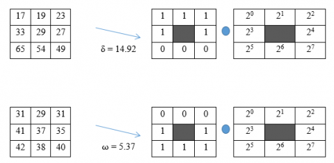
Noisy pixel identification plays a major role in denoising filter to improve the efficiency. The ability to protect the edge is completely dependent on the noisy pixel detection [29]. The mismatch between noise free pixels and noisy pixels results in a deterioration of filters' efficiency [30]. The level of noise effects the original pixels and produces a minimum or maximum grey value (0 or 255) [31]. Some images may have a grey value of 0 and 255 in original pixels. These original pixels may be misclassified as the noisy pixels and the denoising filters may decrease their efficiency [32]. The minimum, medium and maximum value of pixels in the processing window is used in this three-value filter to characterise the pixel class and to rebuild noisy pixels [33]. A window size 3 * 3 is added to a noisy picture in this filter. The window shifts from top to bottom and from right to left. The similitude between noisy pixel and noise free pixels is measured. The processing window PWx,y is used for a given noisy image data. For the reconstruction of noisy pixels, two extreme values 0 and 255 are omitted. The updated picture is obtained as
$\begin{align} & \operatorname{Im}age(p,q)=\operatorname{Im}age(X,Y)\,if\,\operatorname{Im}age(X,Y)\ne 0\, \\ & and\,I \\ & mage(X,Y)\ne 255 \\\end{align}$
If in the processing window the central pixel is equal to the minimum or the maximum grey colour, then the next pixel is tested and reconstructed [34]. In the local processing window the maximum and minimum pixel value (PWx,y) applied to the filter controller is computed as,
$\begin{align} & f{{W}_{\min }}=\min (P{{W}_{x,y}}) \\ & f{{W}_{\max }}=\max (P{{W}_{x,y}}) \\\end{align}$ (1)
The standard denoising problem of complete variance (CV) of an image can be calculated as:
$CV(\operatorname{Im}age(p,q))={{\min }_{y}}\left[ \operatorname{Im}age(x,y)+\lambda *CV(x) \right]$ (2)
$\lambda (t)=\left\{ \begin{matrix}1 \\ -1 \\ 0 \\\end{matrix} \right.\,\,\,\,\,\begin{matrix} 0\le t\le \frac{1}{2}, \\ \frac{1}{2}\le t\le 1, \\ otherwise. \\\end{matrix}$ (3)
where, $\lambda(\mathrm{t})$ is the filter wavelet for noise recognition.
3.1 Auto encoder for image denoising
A large data distribution auto encoder can be viewed as a optimization method which can be used to extract and learn main components [35]. It is mainly considered as a deep learning technique, since it has the capacity to build a deeper network, that can manage the network structure [36] to match the desired environment that is typically used to remove pictures, compress, de-noise, etc. This technique was used as a denoising technique in this research. Auto encoder can be considered the best image classification pre-processing technique using a deep neural network [20].
The eigen values are calculated from the brain image as:
EV=˄R
where, R is the principal component analysis matrix of each eigen vector.
Image(x,y)= [ R(x1 . y1 ) ⋯ R(x2.y2)+N]+λ
When it comes to reducing the dimensionality of a picture, auto encoders rely on neural networks. Using less neurons in the larger layer compared to the input layer, they can refill the input data and minimise the dimensionality [37]. For a deep auto encoder, numerous encoder layers are combined with an unsupervised learning criterion that is taught separately. With labelling data and a classification layer, the pretrained encoder can be enhanced even more. Because the input is so large, an additional hidden intermediate layer is contemplated for encoding and decoding. Let Xi mathematically show the entry, Hi shows Hidden Layer and Yi shows the output. Let the activation functions are represented as:
hi = fi(WiXi + bi), i = 1 to 4
where, Wi is the weight vector between Xi to H1, H1 to H2 and Yi.
Figure 1. Auto encoder model
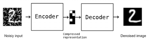
Due to the fact that deep neural networks are nonlinear in nature, no serious challenges should be expected. As a result, it was imperative that the model be pre-trained on noisy data. Figure 1 shows the auto encoder model. Thus, noise was artificially imposed on each layer, increasing efficiency and reducing preparation time. The regular auto encoder's deep network extension can be built on top of a denoising auto encoder. The image has noise applied to it, and the process to remove it is conducted here. Using a noisy image as input, the denoising auto encoder creates a noiseless image as seen in Figure 2.
The concept behind denoising self-encoder is simple. It is used to rebuild data from the ruined/corrupted data input. It is a kind of force effect on the hidden layer, which identifies and prevents solid features. The auto encoder is then trained here to design the input of a corrupted input version. In comparison to the input data, it refines the output. The denoising auto encoder’s training phase is an easy operation. One way of training is to ruin the data sets stochastically, and then feed them to the neural network. On this basis, training is provided to the auto encoder next to the original data set. Another method is to actually delete sections of the data by ruining the data. This would lead to an auto encoder to predict the lack of data. The denoising auto encoders can also stack each other for the process of iterative learning to achieve a balance between input and output.
Figure 2. A Denoising auto encoder
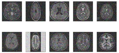
The noisy images of the brain are considered and then after applying the denoising process, the noiseless images have to be generated. The noisy brain images are represented in Figure 3.
Figure 3. Noisy images of brain
The process of denoising the image in the proposed model is explained in the algorithm.
Algorithm Image_De_nosing_Auto_encoder
{
Step-1: Input the image dataset that contain noise values or add noise values to the dataset and provide as Input whose pixel value range is from 0 to 255.
Step-2: From the image extract the pixels that are inside the window that exactly forms the image. The image segmentation and pixel extraction is performed as:
$\begin{align} & Segment(I(P,Q))= \\ & \sqrt{\frac{\sum\nolimits_{i=1}^{N}{{{(\operatorname{Im}age{{(i)}_{i}}-\mu )}^{q}}+{{({{(P+Q)}_{n}})}^{2}}}}{(P+1)+\theta }} \\\end{align}$
$\begin{align} & \mu =\frac{\sum\nolimits_{i=1}^{N}{\operatorname{Im}age{{(I)}_{i}}+Threshold}}{(P+1)}+\theta \\ & +\int\limits_{i}^{N}{\min (\operatorname{Im}age(i+1))} \\\end{align}$ (4)
$\lambda =\frac{\sum\nolimits_{i=1}^{N}{\max (\operatorname{Im}age(P,Q))}}{p*q}+Threshold$ (5)
$\delta =\sqrt{\frac{\sum\nolimits_{i=1}^{p}{{{(\lambda )}^{2}}-Segment(I(i))}}{p(\operatorname{Im}age(i+1))}}+Threshold$ (6)
Here, N is the total pixels in image, ⍬ is the angle of the image, P, Q are the pixels extracted as a set.
Step-3: The mean value is calculated for all pixels in the window calculated as:
$\begin{align} & Mean\_Pixels(P,Q)= \\ & Round\,\left( \frac{\sum\limits_{i=1\,}^{N}{\sum\limits_{j=1}^{N}{\operatorname{Im}age\left( P+\lambda +n \right)}}}{\left( 2P+1 \right)\times \left( 2Q+1 \right)} \right)+\delta \\\end{align}$ (7)
Step-4: After calculating the mean of the pixels, the corrupted pixels in the extracted pixel set from the window is identified. The Corrupted pixels are identified as:
$C{{P}_{P,Q}}=\left\{ \begin{matrix} 1 \\ 0 \\\end{matrix} \right.\,\,\begin{matrix} \begin{align} & {{P}_{ij}}\le X(\min (\delta ))\vee {{x}_{P,Q}} \\ & \ge X(Threshold-Q+1) \\\end{align} \\ other\,wise \\\end{matrix}$ (8)
Step-5: The corrupted pixels are stored in a set for removal of noise using Deep Convolution Neural Networks. The stored is represented as:
Step-6: The auto encoders are considered for processing the noise values and the noise is removed as:
$N{{L}_{p,q}}=\sum\limits_{i=1}^{N}{\sum\limits_{j=1}^{N}{\lambda _{i,j}^{N}\left[ \delta _{i}^{2}+\delta {{(\mu _{j}^{*})}^{2}} \right]}}$ (9)
$\varepsilon \in (0,1)\,and\,\lambda ,\delta >0$
$\begin{align}& Noise\_\operatorname{Re}mova{{l}_{P,Q}}(IS(i))=\sum\limits_{i=0}^{N}{(\operatorname{Im}age(i,i+1))}+\varepsilon \\ & +\,\frac{(Max(NL(\operatorname{Im}age(i)))-Min(NL(\operatorname{Im}age(i+1)))}{\theta *\left( \frac{N-2x+\lambda i}{2} \right)\,!\,\left( \frac{N+2x-\lambda j}{2} \right)} \\\end{align}$ (10)
Step-7: After the noise removal from all the corrupted pixels, the weights for the pixels are calculated for improving the quality and to reduce the unnecessary data. The weights are calculated as:
$\begin{align} & {{W}_{i}}=255- \\ & \left( \frac{\left( Noise\_\operatorname{Re}moval(\operatorname{Im}ag{{e}_{i}})-{{P}_{\min }} \right)\times 254}{{{P}_{\max }}-{{Q}_{\min }}} \right)+\lambda \\\end{align}$ (11)
Step-8: Mean Square error is calculated to identify the performance levels. The MSE is calculated as:
$MSE=\frac{1}{n}\sum\limits_{i}^{n}{{{\left( {{O}_{i}}-{{T}_{i}} \right)}^{2}}}$ (12)
Here, n is the number of samples, $T_{i}$ is the original output, and $O_{i}$ is the predicted output with $i \in[1 . . N]$ .
}
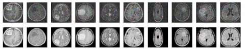
Each layer can be modified in the convolution layer or some previous layers on the other hand can be set while controlling the remaining deeper layers. This is driven by the awareness of the fact that the corrupted pixels seem to be increasingly non-exclusive, including, for example, pixels such as edge contents. Fully connected layers’ equals in a customary neural system where each unit of perception reflects on the input of all units from the layer and results in the final layer for all units. The images after noise removal is represented in Figure 4.
Figure 4. Noisy images and noiseless images
The proposed model is implemented in ANACONDA using python programming. The dataset is considered from the link https://www.kaggle.com/navoneel/brain-mri-images-for-brain-tumor-detection. Different experimental findings on the specific dataset have validated the proposed model. The dataset has 23555 images of brain tumour. The Python framework with some simple packages including NumPy, SciPy and matplotlib was considered for an experimental purpose. The proposed auto encoder was compared with traditional Convolutional Denoising Auto encoder (CDA) model to validate our experiment. The proposed model is compared with the traditional method with the parameters Image Segmentation Time Levels, Pixel Extraction Time Levels, Noise Removal Time Levels, Accuracy Levels in Noise Removal and PSNR Levels.
In order to determine the efficiency of the proposed system, multiple measurement criteria’s are used. The metrics consists of group of esteems that includes standard primary evaluating methods. The assessment metrics used includes True Positive, True Negative, False Positive and False Negative, Sensitivity, Specificity and Accuracy.
$Sensitivity\,\,\,\,=\,\,\,\frac{\text{T(P)}}{\text{T(P)}+\text{F(N)}}\,\,\,\,\,\,\,$ (13)
$Specificity\,\,\,\,=\,\,\,\frac{\text{T(N)}}{\text{F(P)}+\text{T(N)}}\,\,\,\,\,\,$ (14)
$Accuracy\,\,\,\,=\,\,\,\frac{\text{T(P)}+\text{T(N)}}{\text{T(P)}+\text{F(N)}+\text{F(P)}+\text{T(N)}}\,\,\,$ (15)
Image segmentation is a central subject in image and computer vision processing, including scene interpretation, medical image analysis, robotic perception, video monitoring, enhanced reality and compression. Different technologies have been applied in the literature for image segmentation. Recently there has been a large number of projects aimed at developing image-segmentation approaches using deep learning models because of the success of deep learning models in a wide variety of vision applications. The segmentation of images leads to more granular knowledge on the structure of an image and hence an enhancement of the object detection principle. The proposed model segmentation time levels are contrasted with the existing model and the time levels are indicated in Figure 5.
Figure 5. Image segmentation time levels
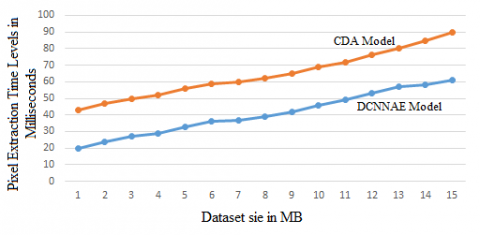
Figure 6. Pixel extraction time levels
Deep Learning using CNN plays a significant role in the image processing field, particularly medical image processing and computer-aided diagnosis, since artefacts such as lesions and organs cannot be described accurately by a simple equation; therefore, medical pattern recognition basically involve “learning from examples.” One of the most common uses of deep learning model is to classify objects such as lesions in certain groups based on input characteristics of segmented object candidates. The inputs in the neural filter are an object pixel value and adjacent pixel values in a sub region or local window. The neural filter output is a value of one pixel. The pixel extraction time levels of the proposed and the existing models are illustrated in Figure 6.
The performance levels of the proposed and traditional models are indicated in Table 1. The accuracy, specificity and sensitivity levels of the proposed and existing models are indicated in Table 1.
Table 1. Performance levels
|
Classification Techniques |
Accuracy |
Specificity |
Sensitivity |
|
MLPNN |
0.75 ± 0.31 |
0.81±0.28 |
0.81±0.27 |
|
RBFNN |
0.71±0.29 |
0.70±0.21 |
0.78±0.31 |
|
ELM |
0.82±0.17 |
0.82±0.27 |
0.87±0.19 |
|
PNN |
0.78±0.16 |
0.86±0.22 |
0.82±0.23 |
|
CDA |
0.83±0.27 |
0.73±0.27 |
0.84±0.21 |
|
Proposed DCNNAE |
0.91±0.15 |
0.93±0.15 |
0.95±0.23 |
During image acquisition, coding, transmission and processing steps, noise is often present in digital pictures. Without previous knowledge of filtering techniques, it is difficult to eliminate noise from digital images. This noise disturbs the picture or video signal. Image de-noising is a critical processing operation, as both a process itself and a part for other processes. A picture can be de-noised in several ways. The essential property of a good model for denoising the image is to minimise noise and to retain edges as much as possible. The Denoising time levels of the proposed and existing models are indicated in Figure 7.
The accuracy levels in denoising of images and getting a clear image of the proposed and existing models are indicated in Figure 8.
Figure 7. Denoising time levels
Figure 8. Accuracy levels in noise removal
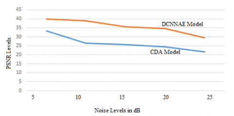
The PSNR is the ratio of the maximum image power possible to the power of noise, which affects the accuracy of its representation. In order to estimate a picture's PSNR, the image needs to be compared to a perfect clean image at maximum capacity. The PSNR levels are illustrated in Table 2 and Figure 9.
Table 2. PSNR levels
|
Noise Level dB |
Existing CDA Model |
Proposed DCNNAE Model |
|
5 |
33.21 |
39.86 |
|
10 |
26.45 |
38.78 |
|
15 |
25.67 |
35.53 |
|
20 |
24.32 |
34.47 |
|
25 |
21.57 |
29.54 |
Figure 9. PSNR levels
The loss levels and accuracy levels of the proposed model is indicated in Figure 10. The results show that the proposed model accuracy rate is high than the traditional methods.
Figure 10. Loss and accuracy levels
Auto encoder is a good choice because of its use in denoising, which has a lot of potential in terms of feature extraction and data part comprehension as the first steps before diving into image analysis and processing. The Denoising Auto encoder (DAE) method involves adding noise to the input image to corrupt the data and mask some of the values, then reconstructing the image. The DAEs learn the input features during image reconstruction, resulting in better latent representation extraction overall. Because of the idea of input corruption before it is considered, the D noising Auto encoder has a lower probability of learning identity feature than the auto encoder. Denoising is recommended for training the model, and DAEs help the model in two ways: first, they retain the input information, and second, they try to eliminate the noise added by the auto-encoder. Denoising Auto encoders have been shown in natural image patches and digit images to be edge and larger stroke detectors, respectively. Since noise contamination may come from a variety of sources, with varying intensities and durations, the picture becomes hazy and unclear. It is no longer possible to restore the original image using a single process. As a result, the proposed model uses a DCNN based Auto Encoder to perform image denoising. In the future, image compression can be used in a variety of ways to minimise image size. The segmentation of these reduced images is then done using probabilistic, model-based segmentation for better noise removal and reducing the time complexity in noise reduction.
[1] Kermi, A., Mahmoudi, I., Khadir, M.T. (2018). Deep convolutional neural networks using U-Net for automatic brain tumor segmentation in multimodal MRI volumes. In International MICCAI Brainlesion Workshop, pp. 37-48. https://doi.org/10.1007/978-3-030-11726-9_4
[2] Mallick, P.K., Ryu, S.H., Satapathy, S.K., Mishra, S., Nguyen, G.N., Tiwari, P. (2019). Brain MRI image classification for cancer detection using deep wavelet autoencoder-based deep neural network. IEEE Access, 7: 46278-46287. https://doi.org/10.1109/ACCESS.2019.2902252
[3] Afshar, P., Shahroudnejad, A., Mohammadi, A., Plataniotis, K.N. (2018). Carisi: Convolutional autoencoder-based inter-slice interpolation of brain tumor volumetric images. In 2018 25th IEEE International Conference on Image Processing (ICIP), pp. 1458-1462. https://doi.org/10.1109/ICIP.2018.8451759
[4] Naz, S., Hameed, I.A. (2017). Automated techniques for brain tumor segmentation and detection: A review study. In 2017 International Conference on Behavioral, Economic, Socio-cultural Computing (BESC), pp. 1-6. https://doi.org/10.1109/BESC.2017.8256397
[5] Ferlay, J., Soerjomataram, I., Dikshit, R., Eser, S., Mathers, C., Rebelo, M. (2015). Cancer incidence and mortality worldwide: Sources, methods and major patterns in GLOBOCAN 2012. International Journal of Cancer, 136(5): E359-E386. https://doi.org/10.1002/ijc.29210
[6] Fiçici, C.Ö., Eroğul, O., Telatar, Z. (2017). Fully automated brain tumor segmentation and volume estimation based on symmetry analysis in MR images. In CMBEBIH 2017, pp. 53-60. https://doi.org/10.1007/978-981-10-4166-2_9
[7] Uma, K., Suhasini, K., Vijayakumar, M. (2016). A comparative analysis of brain tumor segmentation techniques. Indian Journal of Science and Technology.
[8] Patil, R.C., Bhalchandra, A.S. (2012). Brain tumour extraction from MRI images using MATLAB. International Journal of Electronics, Communication and Soft Computing Science & Engineering (IJECSCSE), 2(1): 1.
[9] Junejo, A.Z., Memon, S.A., Memon, I.Z., Talpur, S. (2018). Brain tumor segmentation using 3d magnetic resonance imaging scans. In 2018 1st International Conference on Advanced Research in Engineering Sciences (ARES), pp. 1-6. https://doi.org/10.1109/ARESX.2018.8723285
[10] Jemimma, T.A., Vetharaj, Y.J. (2018). Watershed algorithm based DAPP features for brain tumor segmentation and classification. In 2018 International Conference on Smart Systems and Inventive Technology (ICSSIT), pp. 155-158. https://doi.org/10.1109/ICSSIT.2018.8748436
[11] Oo, S.Z., Khaing, A.S. (2014). Brain tumor detection and segmentation using watershed segmentation and morphological operation. International Journal of Research in Engineering and Technology, 3(3): 367-374.
[12] Myronenko, A. (2018). 3D MRI brain tumor segmentation using autoencoder regularization. In International MICCAI Brainlesion Workshop, pp. 311-320. https://doi.org/10.1007/978-3-030-11726-9_28
[13] He, K., Zhang, X., Ren, S., Sun, J. (2016). Identity mappings in deep residual networks. In European Conference on Computer Vision, pp. 630-645. https://doi.org/10.1007/978-3-319-46493-0_38
[14] He, K., Zhang, X., Ren, S., Sun, J. (2015). Delving deep into rectifiers: Surpassing human-level performance on ImageNet classification. In Proceedings of the IEEE International Conference on Computer Vision, pp. 1026-1034.
[15] Milletari, F., Navab, N., Ahmadi, S. A. (2016). V-net: Fully convolutional neural networks for volumetric medical image segmentation. In 2016 Fourth International Conference on 3D Vision (3DV), pp. 565-571. https://doi.org/10.1109/3DV.2016.79
[16] Sudre, C.H., Li, W., Vercauteren, T., Ourselin, S., Cardoso, M.J. (2017). Generalised dice overlap as a deep learning loss function for highly unbalanced segmentations. In Deep Learning in Medical Image Analysis and Multimodal Learning for Clinical Decision Support, pp. 240-248. https://doi.org/10.1007/978-3-319-67558-9_28
[17] Ezhilarasi, R., Varalakshmi, P. (2018). Tumor detection in the brain using faster R-CNN. In 2018 2nd International Conference on I-SMAC (IoT in Social, Mobile, Analytics and Cloud), pp. 388-392. https://doi.org/10.1109/I-SMAC.2018.8653705
[18] Krizhevsky, A., Sutskever, I., Hinton, G.E. (2012). ImageNet classification with deep convolutional neural networks. Advances in Neural Information Processing Systems, 25: 1097-1105.
[19] Thaha, M.M., Kumar, K.P.M., Murugan, B.S., Dhanasekeran, S., Vijayakarthick, P., Selvi, A.S. (2019). Brain tumor segmentation using convolutional neural networks in MRI images. Journal of Medical Systems, 43(9): 1-10. https://doi.org/10.1007/s10916-019-1416-0
[20] Akkalakshmi, M., Riyazuddin, Y.M., Revathi, V., Pal, A. (2020). Autoencoder-based feature learning and up-sampling to enhance cancer prediction. International Journal of Future Generation Communication and Networking, 13(1): 1453-1459.
[21] Shreyas, V., Pankajakshan, V. (2017). A deep learning architecture for brain tumor segmentation in MRI images. In 2017 IEEE 19th International Workshop on Multimedia Signal Processing (MMSP), pp. 1-6. https://doi.org/10.1109/MMSP.2017.8122291
[22] Singh, M., Verma, A., Sharma, N. (2018). An optimized cascaded stochastic resonance for the enhancement of brain MRI. Irbm, 39(5): 334-342. https://doi.org/10.1016/j.irbm.2018.08.002
[23] Pham, T. X., Siarry, P., Oulhadj, H. (2018). Integrating fuzzy entropy clustering with an improved PSO for MRI brain image segmentation. Applied Soft Computing, 65: 230-242. https://doi.org/10.1016/j.asoc.2018.01.003
[24] Tong, J., Zhao, Y., Zhang, P., Chen, L., Jiang, L. (2019). MRI brain tumor segmentation based on texture features and kernel sparse coding. Biomedical Signal Processing and Control, 47: 387-392. https://doi.org/10.1016/j.bspc.2018.06.001
[25] LeCun, Y., Bengio, Y., Hinton, G. (2015). Deep learning. Nature, 521(7553): 436-444. https://doi.org/10.1038/nature14539
[26] Satapathy, S.K., Jagadev, A.K., Dehuri, S. (2015). An empirical analysis of training algorithms of neural networks: a case study of EEG signal classification using java framework. In Intelligent Computing, Communication and Devices, pp. 151-160. https://doi.org/10.1007/978-81-322-2009-1_18
[27] Mishra, S., Mishra, D. (2015). SVM-BT-RFE: An improved gene selection framework using Bayesian T-test embedded in support vector machine (recursive feature elimination) algorithm. Karbala International Journal of Modern Science, 1(2): 86-96. https://doi.org/10.1016/j.kijoms.2015.10.002
[28] Jyoti, A., Mohanty, M.N., Kumar, M.P. (2014). Morphological based segmentation of brain image for tumor detection. In 2014 International Conference on Electronics and Communication Systems (ICECS), pp. 1-5. https://doi.org/10.1109/ECS.2014.6892750
[29] Abraham, B., Nair, M.S. (2018). Computer-aided diagnosis of clinically significant prostate cancer from MRI images using sparse autoencoder and random forest classifier. Biocybernetics and Biomedical Engineering, 38(3): 733-744. https://doi.org/10.1016/j.bbe.2018.06.009
[30] Despotović, I., Goossens, B., Philips, W. (2015). MRI segmentation of the human brain: Challenges, methods, and applications. Computational and mathematical methods in Medicine. https://doi.org/10.1155/2015/450341
[31] Allaoui, A.E., Mohammed, M. (2018). Evolutionary region growing for image segmentation. International Journal of Applied Engineering Research, 13(5): 2084-2090.
[32] Hiralal, R., Menon, H.P. (2016). A survey of brain MRI image segmentation methods and the issues involved. In the International Symposium on Intelligent Systems Technologies and Applications, pp. 245-259.
[33] Yazdani, S., Yusof, R., Karimian, A., Pashna, M., Hematian, A. (2015). Image segmentation methods and applications in MRI brain images. IETE Technical Review, 32(6): 413-427. https://doi.org/10.1080/02564602.2015.1027307
[34] Xiao, J., Tong, Y. (2014). Research of brain MRI image segmentation algorithm based on FCM and SVM. In the 26th Chinese Control and Decision Conference (2014 CCDC), pp. 1712-1716. https://doi.org/10.1109/CCDC.2014.6852445
[35] Nayak, S.K., Karali, Y., Panda, S.C. (2015). A study on brain MRI image segmentation techniques. Int. J. Res. Stud. Comput. Sci. Eng., 2(9): 4-13.
[36] Chen, M., Yan, Q., Qin, M. (2017). A segmentation of brain MRI images utilizing intensity and contextual information by Markov random field. Computer Assisted Surgery, 22(sup1): 200-211. https://doi.org/10.1080/24699322.2017.1389398
[37] Jose, A., Ravi, S., Sambath, M. (2014). Brain tumor segmentation using k-means clustering and fuzzy c-means algorithms and its area calculation. International Journal of Innovative Research in Computer and Communication Engineering, 2(3): 3496-3501.