Omar Barkat*![]() | Hamza Mihoubi
| Hamza Mihoubi![]() | Awatif Muflih Alqahtani
| Awatif Muflih Alqahtani![]()
© 2025 The authors. This article is published by IIETA and is licensed under the CC BY 4.0 license (http://creativecommons.org/licenses/by/4.0/).
OPEN ACCESS
Using the Homotopy Perturbation Laplace Transform Method (HPLTM), the objective of our current work is to find the analytical solution of the nonlinear fractional partial differential equations arising in the spatial diffusion model of biological populations. This is achieved by replacing the Caputo fractional derivative of the Riemann-Liouville model with the Catogambola fractional derivative represented in the Caputo type. Moreover, the homotopy perturbation transform technique integrates the Laplace transform with the homotopy perturbation method. In addition, the efficiency of the proposed method is verified through three test examples. Accordingly, the results obtained by applying the proposed method for different fractional orders are plotted, and a comparative analysis is performed between our results and those of previous studies.
Caputo-Katugampola fractional derivative, Homotopy Perturbation Laplace Transform Method, Mittag-Leffler function, fractional biological population model
Fractional calculus is a fundamental branch of mathematics, used to calculate arbitrary derivatives and integrals. The proven applications of fractional differential equations in various scientific and technical fields have contributed to increasing their importance and popularity. In this respect, fractional derivatives may be utilized to describe nonlinear oscillations in signal processing, electrochemistry, earthquakes, electromagnetism, fluid mechanics, and in fact, diffusion processes. Further, a wide range of physics and engineering issues, including mathematical biology and various chemical process models are addressed using fractional differential equations [1-7]. Since most physical systems are nonlinear in nature, nonlinear problems have proven of great importance to mathematicians, physicists, and engineers. Although it is not always easy to solve nonlinear equations, they lead to interesting phenomena such as chaos and others. Furthermore, recent developments in numerical symbolic computing tools and computer technology in general have helped many scientists, whether mathematicians or physicists, to find numerical solutions to such equations. Numerous appropriate numerical and analytical techniques were used, like the homotopy analysis (HA) method [8, 9], homotopy perturbation (HP) method [10-14], residual power series (RPS) method [15-18], differential transform (DT) method [19-21], Adomian decomposition (AD) method [22-24], and various other approaches. Nevertheless, further information on fractional differential equations can be found in references [25-27].
In this context, we note that the HP method, first developed by He [28-30] is one of the most widely applied analytical methods, because it directly addresses the problem without requiring any kind of transformation, linearization, or differentiation. However, the Laplace transform has shown to be a widely used mathematical technique for solving differential equations. Undoubtedly, transforms are useful in solving many mathematical problems, especially when reformulating the problem to facilitate its solution. Nevertheless, the inverse transformation is useful in finding a solution to the given problem. Furthermore, the Laplace transform and the AD method were combined under Caputo-Katugampola memory [31] for the purpose of generating approximate solutions of the fractional Berger’s equation. As a consequence, numerous physical phenomena have been represented by means of nonlinear partial differential equations, for instance, the partial differential equations arising from the geographic spread of biological populations defined as:
${ }_t^{C K} \mathbb{D}_a^{\alpha, \rho} U(x, y, t)=\frac{\partial^2 U^2}{\partial x^2}+\frac{\partial^2 U^2}{\partial y^2}+f(U)$ (1)
where, $t \geq 0, x, y \in \mathbb{R}$, and $0<\alpha \leq 1, \rho \in \mathbb{R}^{+}$.
Based on initial condition $U(x, y, 0)=\psi_0(x, y)$, where U denotes the population density and ${ }_t^{C K} \mathbb{D}_a^{\alpha, \rho}=\frac{d^\alpha}{d t^\alpha}$ Katugampola fractional derivative in Caputo type order $\alpha$ and $f(U)=l U^a\left(1-h U^b\right)$ represents the population supply due to births and deaths, where, $l, a, h, b$ are real numbers, then Eq. (1) leads to Malthusian and Verhulst laws [32]. Specifically, for $\alpha=1$, the generalized time-fractional biological population model equation reduces to the classical generalized biological population model equation.
Definitely, the fractional biological equations may be resolved using a variety of techniques, including the HA method [33] along with the HP method [34]. For use, nonlinear problems have been solved using the optimum homotopy analysis (OHA) technique [35] and the generalized Laplace homotopy perturbation (GLHP) method under Caputo-Katugampola memory to solve fractional Burger equation and fractional Schrodinger-KdV equation [36]. Inclusive of the HAT method, which stands for a combination of the Laplace transform (LT) and HA methods, for solving the generalized biological population models [37]. Additionally, the Elzaki transform homotopy perturbation (ETHP) represents a combination of the HP and Elzaki transform (ET) methods [38]. Likewise, AD method is presented for finding purpose of the exact solutions of more general biological population models [1]. The solution of some biological population models of non-integer order, a novel technique identified as iterative Laplace transform (ILT) has been used [39]. In addition, generalized fractional biological population model has been solved by using ILT method [40]. However, due to the challenges posed by nonlinear variables, a number of strategies have been applied; including the numerical Laplace transform approach for the approximate solution of a class of nonlinear differential equations based on the decomposition method [41]. The variational iteration method and Adomian decomposition method have been used to solve the nonlinear partial differential equations arising in the biological populations [42]. The q-homotopy analysis generalized transforms method (q-HAGTM) and generalized Laplace decomposition (GLD) method by substituting the time derivative with the Katugampola fractional [43], the Sumudu decomposition (SD) method [44], and the homotopy perturbation Sumudu transform (HPST) method [45] have recently been put forth to address such nonlinearities. In light of which, these approaches have resulted in highly efficient methods for handling a wide range of nonlinear problems.
In this study, we apply the Caputo-Katugampola fractional derivative for application purpose of the homotopy perturbation $\rho-$Laplace transform (HPLT) method in order to obtain the numerical and analytical solutions of the fractional biological population models. Besides, the HPLT method is the LTHP method, which represents a combined form of the LT and HP methods. The numerical results are then displayed through illustrations. The answer is given by the suggested methods in a rapidly converging series, which might eventually lead to an exact and approximate solution. On the other hand, these techniques have the benefit of combining two effective approaches for provision purpose of both precise and approximate solutions for nonlinear equations.
The manuscript's structure is as follows: Section 2 covers the basic concepts related to the Caputo-Katugampola fractional derivative and the $\rho-$Laplace transform, which are relevant to the problems under discussion. Section 3 explains the HPLT approach to deriving solutions to the fractional-time biological population model. Section 3 is devoted to applying our approach to time-fractional biological population models to verify the accuracy and effectiveness of these models. In this context, we present the results through numerical and graphical analyses. We end this study with some concluding remarks in Section 5.
This section examines the primary definitions and properties of fractional calculus theory, which have been utilized throughout this paper.
Definition 2.1 [46]. Let $\alpha \in \mathbb{C}, \rho \in \mathbb{R}^{+}, a<t<b$, and consider a finite (or infinite) interval on the positive half-axis $(0<a<b<\infty)$, within the real numbers $\mathbb{R}^{+}$. The Katugampola fractional integrals of order $\alpha$ are defined by:
$\mathfrak{J}_a^{\alpha ; \rho} \psi(t)=\frac{1}{\Gamma(\alpha)} \int_a^t\left(\frac{t^\rho-x^\rho}{\rho}\right)^{\alpha-1} \psi(x) \frac{d x}{x^{1-\alpha}}$ (2)
$\Im_b^{\alpha ; \rho} \psi(t)=\frac{1}{\Gamma(\alpha)} \int_t^b\left(\frac{x^\rho-t^\rho}{\rho}\right)^{\alpha-1} \psi(x) \frac{d x}{x^{1-\alpha}}$ (3)
The Caputo-type modification of left-sided and right-sided Katugampola fractional derivative is given by:
Theorem 2.1 [47]. Let $\Re(\alpha) \geq 0, n=[\Re(\alpha)]+1$, and consider $(0<a<b<\infty)$. If $\psi \in A C_\delta^n([a, b])$, where $A C[a, b]$ represents the spaces of absolutely continuous functions on [a, b], such that
$A C_\delta^n([a, b])=\left\{g:[a, b] \rightarrow \mathbb{C}: \delta^{n-1} g(x) \in A C[a, b], \delta=x^{1-\rho} \frac{d}{x}\right\}$
Then, ${ }_t^K \mathbb{D}_a^{\alpha, \rho} \psi(t)$ and ${ }_t^K \mathbb{D}_b^{\alpha, \rho} \psi(t)$ exists in $[\mathrm{a}, \mathrm{b}]$, and
$\begin{gathered}{ }_t^K \mathbb{D}_a^{\alpha, \rho} \psi(t)=(\delta)^n \mathfrak{J}_a^{n-\alpha ; \rho} \psi(t) = \frac{(\delta)^n}{\Gamma(n-\alpha)} \int_a^t\left(\frac{t^\rho-x^\rho}{\rho}\right)^{n-\alpha-1} \psi(x) \frac{d x}{x^{1-\rho}}\end{gathered}$ (4a)
${ }_t^K \mathbb{D}_b^{\alpha, \rho} \psi(t)=(-\delta)^n \mathfrak{J}_b^{n-\alpha ; \rho} \psi(t)=\frac{(-\delta)^n}{\Gamma(n-\alpha)} \int_t^b\left(\frac{x^\rho-t^\rho}{\rho}\right)^{n-\alpha-1} \psi(x) \frac{d x}{x^{1-\rho}}$ (4b)
Theorem 2.2 [47]. The Caputo-type fractional derivatives, both left and right-sided, with complex order $\alpha$, $\Re(\alpha) \geq 0$ and $\rho$ belonging to the set of positive real numbers, are provided as follows, respectively:
${ }_t^{C K} \mathbb{D}_a^{\alpha, \rho} \psi(t)=\mathfrak{J}_a^{n-\alpha ; \rho}(\delta)^n \psi(t)=\frac{1}{\Gamma(n-\alpha)} \int_a^t\left(\frac{t^\rho-x^\rho}{\rho}\right)^{n-\alpha-1}(\delta)^n \psi(x) \frac{d x}{x^{1-\rho}}$ (5)
${ }_t^{C K} \mathbb{D}_b^{\alpha, \rho} \psi(t)=\Im_b^{n-\alpha ; \rho}(-\delta)^n \psi(t)=\frac{1}{\Gamma(n-\alpha)} \int_t^b\left(\frac{x^\rho-t^\rho}{\rho}\right)^{n-\alpha-1}(-\delta)^n \psi(x) \frac{d x}{x^{1-\rho}}$ (6)
Here, $\delta=t^{1-\rho} \frac{d}{t}$ and $\rho>0$.
In particular, for $\rho=1$ and for $\rho \rightarrow 0^{+}$, we obtain the Riemman-Liouville fractional derivative and the Hadamard fractional derivative, respectively.
Theorem 2.3 [47]. Let $\psi \in C([a, b]), \alpha>\beta>0$ and $\rho>0, a<t<b$, then
${ }_t^K \mathbb{D}_{a+}^\alpha \mathfrak{J}_{a+}^\alpha \psi(t)=\psi(t)$ (7)
As shown below, the Katugampola fractional derivative does not act as the true inverse of the Katugampola fractional integral.
Theorem 2.4 [47]. Let $\mathfrak{J}_{a+}^{n-\alpha} \psi \in A C^n([a, b])$, and $n-1<\alpha \leq n, \rho>0, n \in \mathbb{N}$, then
$\mathfrak{I}_{a+}^{\alpha, \rho}{}^K_t \mathbb{D}_a^{\alpha, \rho} \psi(t)=\psi(t)-\sum_{k=0}^{n-1} c_k\left(\frac{t^\rho-a^\rho}{\rho}\right)^{k-n+\alpha}$ (8)
with $c_k$ are real constants.
Definition 2.2 [47]. Let $\alpha, m>0$. The one-parameter Mittag-Leffler function has the power series representation:
$E_{\alpha, m}(t)=\sum_{m=0}^{\infty} \frac{t^m}{\Gamma(m \alpha+1)}$ (9)
with $\Gamma(.)$ is gamma function.
Definition 2.3 [48]. The $\rho-$ Laplace transform of the function $\psi$ is given by:
$G(s)=\mathcal{L}_\rho[\psi(t)]=\int_0^{+\infty} e^{-s \frac{t^\rho}{\rho}} \psi(t) \frac{d t}{t^{1-\rho}}, \rho>0$ (10)
where, $\psi:[0, \infty) \rightarrow \mathbb{R}$ is a real valued function.
The inverse modified $\rho$-Laplace transform is given by:
$\psi(t)=\mathcal{L}_\rho^{-1}[G(s)]=\frac{1}{2 \pi i} \int_{c-i \infty}^{c+i \infty} e^{-s \frac{t^\rho}{\rho}} G(s) \frac{d s}{s}$ (11)
where, $c=\Re(s), t \in(a, \infty), a>0$.
Theorem 2.5 [48]. Let the function $\psi$ be continuous and of exponential order $e^{-c \frac{t^\rho}{\rho}}$ such that $\delta \psi(t)$ has shown to be piecewise continuous over every single finite interval $[0, \mathrm{t}]$, subsequently, $\rho$-Laplace transform of $\delta \psi(t)$ exists for $s> c$, and
$\mathcal{L}_\rho[\delta \psi(t)](s)=s \mathcal{L}_\rho[\psi(t)](s) \times \psi(0)$ (12)
Definition 2.4 [48]. The $\rho$-Convolution of $\psi$ and $g$ is given by:
$\psi(t) * g(t)=\int_0^t \psi\left(\left(t^\rho-s^\rho\right)^{\frac{1}{\rho}}\right) g(s) \frac{d s}{s^{1-\rho}}$ (13)
Theorem 2.6 [48]. ($\rho-$Convolution theorem)
$\mathcal{L}_\rho\{\psi(t) * g(t)\}=\mathcal{L}_\rho[\psi(t), s] \mathcal{L}_\rho[g(t), s]=F(s) G(s)$ (14)
which equivalently to
$\mathcal{L}_\rho{ }^{-1}\{F(s) G(s), t\}=\psi(t) * g(t)$ (15)
Theorem 2.7 [48]. Let $\alpha>0$ and $\psi$ be a piecewise continuous function on $[0, t]$ and of $\rho$-exponential order $e^{-c \frac{t^\rho}{\rho}}$. Then
$\mathcal{L}_\rho\left\{\Im_a^{\alpha ; \rho} \psi(t), s\right\}=\frac{\mathcal{L}_\rho[\psi(t)]}{s^\alpha}, s>c$ (16)
Theorem 2.8 [48]. Let $\alpha>0$ and $\psi \in A C_\delta^{n-1}[0, a]$ for any $a>0$, and $\delta^k \psi, k=0,1,2, \ldots, n-1$ be of $\rho-$ exponential order $e^{-c \frac{t^\rho}{\rho}}$. Then
$\mathcal{L}_\rho\left\{\left({ }_t^C \mathbb{D}_a^{\alpha, \rho} \psi(t), s\right)\right\}=s^\alpha\left\{\mathcal{L}_\rho\{\psi(t)\}-\sum_{k=0}^{n-1} s^{-k-1}\left(\delta^k \psi\right)(0)\right\}$ (17)
where, $s>c$.
The $\rho-$Laplace transform of the derived Caputo-Catogambula fraction is obtained using the $\rho-$Laplace transform on both sides of Eq. (5) as follows:
$\mathcal{L}_\rho\left\{\left({ }_t^{C K} \mathbb{D}_a^{\alpha, \rho} \psi(t), s\right)\right\}=s^\alpha\left\{\mathcal{L}_\rho\{\psi(t)\}\right\}-\sum_{k=0}^{n-1} s^{\alpha-k-1}\left(\delta^k \psi\right)(0)$ (18)
Lemma 1 [48, 49]. $\Re(\alpha)>0$ and $\left|\frac{\lambda}{s^\alpha}\right|<1$, the $\rho-$Laplace transform of some special functions are:
To illustrate the concept of the HPLT method, we consider the following non-homogeneous fractional-order nonlinear partial differential equation with its initial condition.
${ }_t^{C K} \mathbb{D}_0^{\alpha, \rho} \psi(x, y, t)+R \psi(x, y, t)+N \psi(x, y, t)=g(x, y, t)$ (19)
such that $0<\alpha \leq 1$,
$\psi(x, y, 0)=h(x, y)$ (20)
where, ${ }_t^{C K} \mathbb{D}_0^\alpha \psi(x, y, t)$ is the derivative of $\psi(x, y, t)$ in the Caputo sense, where, $R$ and $N$ denote linear and nonlinear differential operators, respectively, and $g(x, y, t)$ represents the source term. Additionally, when applying the LT method to both sides of Eq. (19), we get:
$\mathcal{L}_\rho\left\{{ }_t^{C K} \mathbb{D}_a^{\alpha, \rho} \psi(x,, y, t)+R \psi(x, y, t)+N \psi(x, y, t)\right\}=\mathcal{L}_\rho\{g(x, y, t)\}$ (21)
$\mathcal{L}_\rho\left\{{ }_t^{C K} \mathbb{D}_a^{\alpha, \rho} \psi(x,, y, t)\right\}=\mathcal{L}_\rho\{-R \psi(x, y, t)-N \psi(x, y, t)\}+\mathcal{L}_\rho\{g(x, y, t)\}$ (22)
Now, by using the differential property of the $\rho-$Laplace transform of the fractional derivative, we obtain:
$\mathcal{L}_\rho\left\{{ }_t^{C K} \mathbb{D}_a^{\alpha, \rho} \psi(x, y, t)\right\}=s^\alpha\left\{\mathcal{L}_\rho\{\psi(t)\}\right\}-\sum_{k=0}^{n-1} s^{\alpha-k-1}\left(\delta^k \psi\right)(0)=\mathcal{L}_\rho\{-R \psi(x, y, t)-N \psi(x, y, t)\}+\mathcal{L}_\rho\{g(x, y, t)\}$ (23)
By simplifying Eq. (23), then
$\mathcal{L}_\rho\{\psi(x, y, t)\}=\sum_{k=0}^{n-1} s^{-k-1}\left(\delta^k \psi\right)(0)+\frac{1}{s^\alpha}\left\{\mathcal{L}_\rho\{g(x, y, t)\}-\mathcal{L}_\rho\{R \psi(x, y, t)+N \psi(x, y, t)\}\right\}$ (24)
By using the inverse $\rho-$Laplace transform on both sides in Eq. (24), we find:
$\psi(x, y, t)=G(x, y, t)-\mathcal{L}_\rho^{-1}\left[\frac{1}{s^\alpha}\left\{\mathcal{L}_\rho\{R \psi(x, y, t)+N \psi(x, y, t)\}\right\}\right]$ (25)
where, $G(x, y, t)$ denotes the term derived from the initial condition and source term.
By applying the HP method to Eq. (25), we get:
$\psi(x, y, t)=G(x, y, t)+p\left(\mathcal{L}_\rho^{-1}\left[\frac{1}{s^\alpha}\left\{\mathcal{L}_\rho\{R \psi(x, y, t)+N \psi(x, y, t)\}\right\}\right]\right)$ (26)
The homotopy parameter $p$ is utilized to extend the solution as:
$\psi(x, y, t)=\sum_{n=0}^{\infty} p^n \psi_n(x, y, t)$ (27)
The nonlinear term is analysed as:
$N \psi(x, y, t)=\sum_{n=0}^{\infty} p^n H_n(\psi)$ (28)
where, $H_n(\psi)$ is He’s polynomials which is given by:
$H_n\left(\psi_0, \psi_1, \psi_2, \ldots \psi_n\right)=\frac{1}{n!} \frac{\partial}{\partial p^n}\left[N \sum_{n=0}^{\infty} p^n \psi_n\right]$ (29)
By substituting Eqs. (27) and (28) in Eq. (26), we obtain:
$\sum_{n=0}^{\infty} p^n \psi_n(x, y, t)=G(x, y, t)+p\left(\mathcal{L}_\rho{ }^{-1}\left[\frac{1}{s^\alpha}\left\{\mathcal{L}_\rho\left\{R \sum_{n=0}^{\infty} p^n \psi_n(x, y, t)+N \sum_{n=0}^{\infty} p^n H_n(\psi)\right\}\right\}\right]\right)$ (30)
Comparing the coefficients of the identical powers of p on both sides of the equation above allows us to derive the following equations:
$p^0: \psi_0(x, y, t)=G(x, y, t)$ (31)
$p^1: \psi_1(x, y, t)=\mathcal{L}_\rho^{-1}\left[\frac{1}{s^\alpha}\left\{\mathcal{L}_\rho\left\{R \psi_0(x, y, t)+H_0(\psi)\right\}\right\}\right]$ (32)
$p^2: \psi_2(x, y, t)=\mathcal{L}_\rho^{-1}\left[\frac{1}{s^\alpha}\left\{\mathcal{L}_\rho\left\{R \psi_1(x, y, t)+H_1(\psi)\right\}\right\}\right]$ (33)
$\vdots \quad \quad \quad \vdots$
$p^n: \psi_n(x, y, t)=\mathcal{L}_\rho^{-1}\left[\frac{1}{s^\alpha}\left\{\mathcal{L}_\rho\left\{R \psi_{n-1}(x, y, t)+H_{n-1}(\psi)\right\}\right\}\right]$ (34)
Finally, we find the solution $\psi_n(x, y, t)$ in this manner, which can be written as:
$\psi(x, y, t)=\psi_0(x, y, t)+\psi_1(x, y, t)+\psi_2(x, y, t)+\psi_3(x, y, t)+\cdots$ (35)
The following theorems have proven that the HP method is gaining convergence towards a solution for the time-fractional generalized biological population model equation, as well as the accuracy estimate of the HP method. Consider an opened and bounded domain $\Omega \in \mathbb{R}^n$, and let $T$ be a positive constant with $0<T \leq \infty$. To illustrate the idea of biological population reproduction, let us consider the equation of a partial biological population model, for any $(x, y, t) \in \Omega \times [0, T]$.
Theorem 3.1 [49]. Let $\psi_n(x, y, t)$ be the function in a Banach space $C(\Omega \times[0, T])=\{u / u$ is continuous on $\Omega \times [0, T]\}$ defined by Eq. (35) for any $n \in \mathbb{N}$. The infinite series $\sum_{k=0}^{\infty} \psi_k(x, y, t)$ converges to the solution $\psi$ of Eq. (19) if there exists a constant $0<\mu<1$ such that $\psi_n(x, y, t) \leq \mu \psi_{n-1}(x, y, t)$ for all $n \in \mathbb{N}$. Therefore, $\left\{S_n\right\}_{n=0}^{\infty}$ is a Cauchy sequence in the Banach space $C^n([a, b], \mathbb{R})$. Consequently, the solution $\sum_{k=0}^{\infty} \psi_k(x, y, t)$ converges to $\psi$.
To reduce the approximate solution, we use the theorem below.
Theorem 3.2 [49]. The maximum absolute error of the series solution, defined in Eq. (35) is assessed as follows:
$\left|\psi(x, y, t)-\sum_{k=0}^{\infty} \psi_k(x, y, t)\right| \leq\left(\frac{\mu^{m+1}}{1-\mu}\right)\left\|\psi_0\right\|$ (36)
Through this section, we apply the homotopy perturbation $\rho-$Laplace transform (HPLT) method for the solving time-fractional generalized biological population model of Eq. (1).
4.1 The first application
Consider the equation of the time-fractional generalized biological population model given by:
${ }_t^{C K} \mathbb{D}_a^{\alpha, \rho} U(x, y, t)=\frac{\partial^2 U^2}{\partial x^2}+\frac{\partial^2 U^2}{\partial y^2}-U(1+h U)$ (37)
where, $0<\alpha \leq 1, \rho>0, t \geq 0, x, y \in \mathbb{R}$, IC: $U(x, y, 0)=e^{\left[\frac{1}{2} \sqrt{\frac{h}{2}}(x+y)\right]}$.
By applying the LT method on both sides of Eq. (37), we get:
$\mathcal{L}_\rho\{U(x, y, t)\}=\frac{1}{\mathrm{~s}} \mathrm{e}^{\left[\frac{1}{2} \sqrt{\frac{\mathrm{~h}}{2}}(\mathrm{x}+\mathrm{y})\right]}+\frac{1}{\mathrm{~s}^\alpha}\left\{\mathcal{L}_\rho\left\{\frac{\partial^2 \mathrm{U}^2}{\partial \mathrm{x}^2}+\frac{\partial^2 \mathrm{U}^2}{\partial \mathrm{y}^2}-\mathrm{U}(1+\mathrm{hU})\right\}\right\}$ (38)
The inverse $\rho-$Laplace transform of Eq. (38) implies that:
$U(x, y, t)=e^{\left[\frac{1}{2} \sqrt{\frac{h}{2}}(x+y)\right]}+\mathcal{L}_\rho{ }^{-1}\left[\frac{1}{s^\alpha}\left\{\mathcal{L}_\rho\left\{\frac{\partial^2 U^2}{\partial x^2}+\frac{\partial^2 U^2}{\partial y^2}-U(1+h U)\right\}\right\}\right]$ (39)
Through simplification of Eq. (39), we obtain:
$\mathrm{U}(\mathrm{x}, \mathrm{y}, \mathrm{t})=\mathrm{e}^{\left[\frac{1}{2} \sqrt{\frac{\mathrm{~h}}{2}}(\mathrm{x}+\mathrm{y})\right]}+\mathcal{L}_\rho{ }^{-1}\left[\frac{1}{\mathrm{~s}^\alpha}\left\{\mathcal{L}_\rho\left\{\frac{\partial^2 \mathrm{U}^2}{\partial \mathrm{x}^2}+\frac{\partial^2 \mathrm{U}^2}{\partial \mathrm{y}^2}-\mathrm{U}-\mathrm{hU}^2\right\}\right\}\right]$ (40)
Now, applying the HP method, we obtain:
$\left.\sum_{n=0}^{\infty} p^n U_n(x, y, t)=e^{\left[\frac{1}{2} \sqrt{\frac{h}{2}}(x+y)\right]}\right.+p\left[\mathcal{L}_\rho^{-1}\left[\frac{1}{s^\alpha}\left\{\mathcal{L}_\rho\left\{N \sum_{n=0}^{\infty} p^n H_n(U)-\sum_{n=0}^{\infty} p^n U_n(x, y, t)\right\}\right\}\right]\right]$ (41)
where, $H_n(U)$ are He’s polynomials that signify the nonlinear terms.
$\begin{gathered}H_n(U)=H_n\left(U_0, U_1, U_2, \ldots U_n\right)=\frac{1}{n!} \frac{\partial}{\partial p^n}\left[N \sum_{n=0}^{\infty} p^n U_n\right] \\ n=0,1,2,3, \ldots\end{gathered}$ (42)
Below, we present the He polynomials, whose first components are listed as:
$H_0(U)=\frac{\partial^2 U_0^2}{\partial x^2}+\frac{\partial^2 U_0^2}{\partial y^2}-h U_0^2$
$H_1(U)=2 \frac{\partial^2\left(U_0 U_1\right)}{\partial x^2}+2 \frac{\partial^2\left(U_0 U_1\right)}{\partial y^2}-2 h\left(U_0 U_1\right)$
$H_2(U)=2 \frac{\partial^2\left(U_0 U_2\right)}{\partial x^2}+\frac{\partial^2 U_1^2}{\partial x^2}+2 \frac{\partial^2\left(U_0 U_2\right)}{\partial y^2}+\frac{\partial^2 U_1^2}{\partial y^2}-2 h\left(U_0 U_2\right)-h U_1^2$
$\vdots \quad \quad \quad \vdots$
By calculating the coefficients of the same power of on both sides in Eq. (41), we obtain the results below:
$p^0: U_0(x, y, t)=e^{\left[\frac{1}{2} \sqrt{\frac{h}{2}}(x+y)\right]}$
$p^1: U_1(x, y, t)=\mathcal{L}_\rho^{-1}\left[\frac{1}{s^\alpha}\left\{\mathcal{L}_\rho\left\{H_0(U)-U_0\right\}\right\}\right]=\mathcal{L}_\rho^{-1}\left[\frac{1}{s^\alpha}\left\{\mathcal{L}_\rho\left\{\frac{\partial^2 U_0^2}{\partial x^2}+\frac{\partial^2 U_0^2}{\partial y^2}-h U_0^2-U_0\right\}\right\}\right]$
$=-e^{\left[\frac{1}{2} \sqrt{\frac{h}{2}}(x+y)\right]} \frac{\left(\frac{t^\rho-a^\rho}{\rho}\right)^\alpha}{\Gamma(\alpha+1)}$
$p^2: U_2(x, y, t)=\mathcal{L}_\rho^{-1}\left[\frac{1}{s^\alpha}\left\{\mathcal{L}_\rho\left\{H_1(U)-U_1\right\}\right\}\right]=\mathcal{L}_\rho^{-1}\left[\frac{1}{s^\alpha}\left\{\mathcal{L}_\rho\left\{2 \frac{\partial^2\left(U_0 U_1\right)}{\partial x^2}+2 \frac{\partial^2\left(U_0 U_1\right)}{\partial y^2}-2 h\left(U_0 U_1\right)-U_1\right\}\right\}\right]$
$=e^{\left[\frac{1}{2} \sqrt{\frac{h}{2}}(x+y)\right]} \frac{\left(\frac{t^\rho-a^\rho}{\rho}\right)^{2 \alpha}}{\Gamma(2 \alpha+1)}$
$\left.p^3: U_3(x, y, t)=\mathcal{L}_\rho^{-1}\left[\frac{1}{s^\alpha}\left\{\mathcal{L}_\rho\left\{H_2(U)-U_2\right\}\right\}\right]=\mathcal{L}_\rho^{-1}\left[\frac{1}{s^\alpha}\left\{\mathcal{L}_\rho\left\{2 \frac{\partial^2\left(U_0 U_2\right)}{\partial x^2}+\frac{\partial^2 U_1^2}{\partial x^2}+2 \frac{\partial^2\left(U_0 U_2\right)}{\partial y^2}+\frac{\partial^2 U_1^2}{\partial y^2}-2 h\left(U_0 U_2\right)-h U_1^2-U_2\right\}\right\}\right.\right]$
$=-e^{\left[\frac{1}{2} \sqrt{\frac{h}{2}}(x+y)\right]} \frac{\left(\frac{t^\rho-a^\rho}{\rho}\right)^{3 \alpha}}{\Gamma(3 \alpha+1)}$
Consequently, the solutions $U(x, y, t)$ are written in the form:
$U(x, y, t)=U_0(x, y, t)+U_1(x, y, t)+U_2(x, y, t)+U_3(x, y, t)+\cdots=e^{\left[\frac{1}{2} \sqrt{\frac{h}{2}}(x+y)\right]} e^{-\left(\frac{t^\rho-a^\rho}{\rho}\right)^\alpha}$ (43)
Next, we end by formulating infinite sums using the Mittag-Leffler function, the Eq. (9) becomes:
$U(x, y, t)=e^{\left[\frac{1}{2} \sqrt{\frac{h}{2}}(x+y)\right]} \mathbb{E}_{\alpha, 1}\left(-\left(\frac{t^\rho-a^\rho}{\rho}\right)^\alpha\right)$ (44)
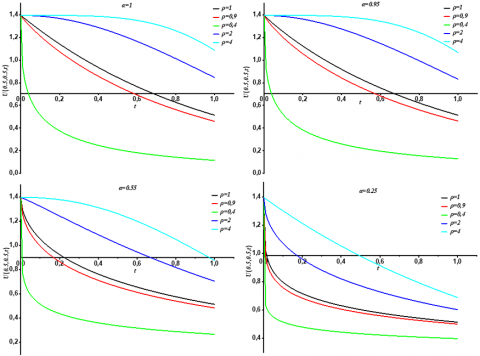
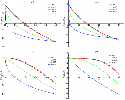
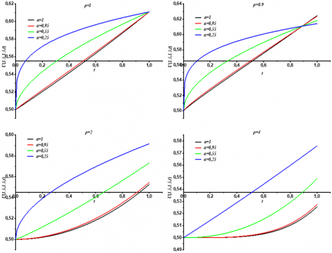
These solutions have shown to be consistent with the solutions found by Devi and Jakhar [38], applying ETHP method and operator the Riemann–Liouville fractional. Besides, the plots of Eq. (43) are depicted in Figures 1-3, for different values of $\alpha=1,0.95,0.55,0.2, \rho=1,0.9,0.4,2,4$, $h=\frac{8}{9}$.
Substituting into Eq. (44) for $\rho=\alpha=1, a=0$, the exact solution of classical biological population model equation is:
$U(x, y, t)=e^{\left[\frac{1}{2} \sqrt{\frac{h}{2}}(x+y)\right]-t}$ (45)
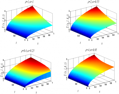
In the model discussed, we performed a simulation analysis to solve the time-fractional generalized biological population model of Eq. (37) via HPLT. Different values of fractional order are taken into consideration for this model such as $\alpha= 1,0.95,0.55,0.2$ for the parameters $\rho=1,0.9,0.4,2,4$. Figures 1-3 explain how $U$ varies with change in fractional order $\alpha$ and $\rho$ time $t$. It evidently demonstrates that with an increase in time $t$ or a decrease in the value of the fractional parameter $\alpha$ and an increase in the value of the fractional parameter $\rho$, a sharp decrease in population density occurs.
Figure 1. The graphs of Eq. (43) for the values of parameter $\rho$, with $h=\frac{8}{9}, a=0, \alpha=1,0.95,0.55,0.25$
Figure 2. The graphs of Eq. (43) for the values of parameter $\alpha$, with $h=\frac{8}{9}, a=0, \rho=1,0.9,0.4,2,4$
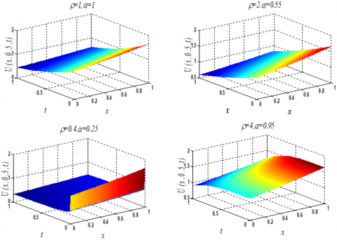
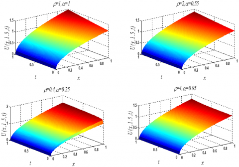
Figure 3. Surface shows the behavior of solution $U(x, y, t)$ of the first application using Eq. (43) with respect to $t$ and $x$, with $(\rho=2, \alpha=0.55),(\rho=1, \alpha=1),(\rho=4, \alpha=0.95),(\rho=0.4, \alpha=0.25)$, and $y=0.5, x=t=0,0.01,1$
4.2 The second application
Consider the following generalized biological population model
$\begin{gathered}{ }_t^{C K} \mathbb{D}_a^{\alpha, \rho} U(x, y, t)=\frac{\partial^2 U^2}{\partial x^2}+\frac{\partial^2 U^2}{\partial y^2}+l U \\ 0<\alpha \leq 1, \rho>0, t \geq 0, x, y \in \mathbb{R}\end{gathered}$ (46)
Using LT method on both sides of Eq. (46), we obtain:
$\mathcal{L}_\rho\{U(x, y, t)\}=\frac{1}{s} \sqrt{x y}+\frac{1}{s^\alpha}\left\{\mathcal{L}_\rho\left\{\frac{\partial^2 U^2}{\partial x^2}+\frac{\partial^2 U^2}{\partial y^2}+l U\right\}\right\}$ (47)
The inverse $\rho-$Laplace transform of Eq. (47) implies that:
$U(x, y, t)=\sqrt{x y}+\mathcal{L}_\rho^{-1}\left[\frac{1}{s^\alpha}\left\{\mathcal{L}_\rho\left\{\frac{\partial^2 U^2}{\partial x^2}+\frac{\partial^2 U^2}{\partial y^2}+l U\right\}\right\}\right]$ (48)
At this time, through applying the HP method, we get:
$\sum_{n=0}^{\infty} p^n U_n(x, y, t)=\sqrt{x y}+p\left[\mathcal{L}_\rho{ }^{-1}\left[\frac{1}{s^\alpha}\left\{\mathcal{L}_\rho\left\{N \sum_{n=0}^{\infty} p^n H_n(U)+l \sum_{n=0}^{\infty} p^n U_n(x, y, t)\right\}\right\}\right]\right]$ (49)
where, $H_n(U)$ are He’s polynomials which indicate the nonlinear terms.
$\begin{gathered}H_n(U)=H_n\left(U_0, U_1, U_2, \ldots U_n\right)=\frac{1}{n!} \frac{\partial}{\partial p^n}\left[N \sum_{n=0}^{\infty} p^n U_n\right] \\ n=0,1,2,3, \ldots\end{gathered}$ (50)
Below, we present the He polynomials, whose first components are listed as:
$H_0(U)=\frac{\partial^2 U_0^2}{\partial x^2}+\frac{\partial^2 U_0^2}{\partial y^2}$
$H_1(U)=2 \frac{\partial^2\left(U_0 U_1\right)}{\partial x^2}+2 \frac{\partial^2\left(U_0 U_1\right)}{\partial y^2}$
$H_2(U)=2 \frac{\partial^2\left(U_0 U_2\right)}{\partial x^2}+\frac{\partial^2 U_1^2}{\partial x^2}+2 \frac{\partial^2\left(U_0 U_2\right)}{\partial y^2}+\frac{\partial^2 U_1^2}{\partial y^2}$
$\vdots \quad \quad \quad \vdots$
By calculating the coefficients of the same power of on both sides in Eq. (49), we obtain the results below:
$p^0: U_0(x, y, t)=\sqrt{x y}$,
$\begin{gathered}p^1: U_1(x, y, t)=\mathcal{L}_\rho{ }^{-1}\left[\frac{1}{s^\alpha}\left\{\mathcal{L}_\rho\left\{H_0(U)+l U_0\right\}\right\}\right]=\mathcal{L}_\rho{ }^{-1}\left[\frac{1}{s^\alpha}\left\{\mathcal{L}_\rho\left\{\frac{\partial^2 U_0^2}{\partial x^2}+\frac{\partial^2 U_0^2}{\partial y^2}+l U_0\right\}\right\}\right] \\ =l \sqrt{x y} \frac{\left(\frac{t^\rho-a^\rho}{\rho}\right)^\alpha}{\Gamma(\alpha+1)}\end{gathered}$
$\begin{gathered}p^2: U_2(x, y, t)=\mathcal{L}_\rho^{-1}\left[\frac{1}{s^\alpha}\left\{\mathcal{L}_\rho\left\{H_1(U)+l U_1\right\}\right\}\right]=\mathcal{L}_\rho^{-1}\left[\frac{1}{s^\alpha}\left\{\mathcal{L}_\rho\left\{2 \frac{\partial^2\left(U_0 U_1\right)}{\partial x^2}+2 \frac{\partial^2\left(U_0 U_1\right)}{\partial y^2}+l U_1\right\}\right\}\right] \\ =l^2 \sqrt{x y} \frac{\left(\frac{t^\rho-a^\rho}{\rho}\right)^{2 \alpha}}{\Gamma(2 \alpha+1)}\end{gathered}$
$\begin{gathered}p^3: U_3(x, y, t)=\mathcal{L}_\rho^{-1}\left[\frac{1}{s^\alpha}\left\{\mathcal{L}_\rho\left\{H_2(U)+l U_2\right\}\right\}\right]=\mathcal{L}_\rho^{-1}\left[\frac{1}{s^\alpha}\left\{\mathcal{L}_\rho\left\{2 \frac{\partial^2\left(U_0 U_2\right)}{\partial x^2}+\frac{\partial^2 U_1^2}{\partial x^2}+2 \frac{\partial^2\left(U_0 U_2\right)}{\partial y^2}+\frac{\partial^2 U_1^2}{\partial y^2}+l U_2\right\}\right\}\right] \\ =l^3 \sqrt{x y} \frac{\left(\frac{t^\rho-a^\rho}{\rho}\right)^{3 \alpha}}{\Gamma(3 \alpha+1)}\end{gathered}$
Consequently, the solutions $U(x, y, t)$ can be formulated as:
$U(x, y, t)=U_0(x, y, t)+U_1(x, y, t)+U_2(x, y, t)+U_3(x, y, t)+\cdots=\sqrt{x y} e^{l\left(\frac{t^\rho-a^\rho}{\rho}\right)^\alpha}$ (51)
Next, we end by formulating infinite sums using the Mittag-Leffler function, the Eq. (9) becomes:
$U(x, y, t)=\sqrt{x y} \mathbb{E}_{\alpha, 1}\left(l\left(\frac{t^\rho-a^\rho}{\rho}\right)^\alpha\right)$ (52)
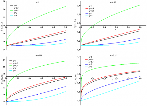
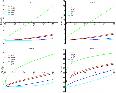
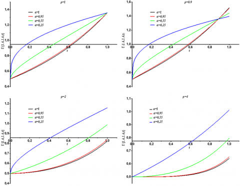
In fact, these solutions agree with the solutions obtained by Liu et al. [34], using HP method and the Riemann-Liouville fractional integration operator. The plots of Eq. (51) are depicted in Figures 4-6, for different values of $\alpha= 1,0.95,0.55,0.2, \rho=1,0.9,0.4,2,4, l=\frac{1}{5}$. By substituting into Eq. (52) for $\rho=\alpha=1, a=0$, the exact solution to the classical generalized biological population model equation is as follows:
$U(x, y, t)=\sqrt{x y} e^{l t}$ (53)
Similarly, in the model discussed, we conducted a simulation analysis to solve the time-fractional generalized biological population model of Eq. (46) via HPLT. Various values of fractional order are taken into account for this model such as $\alpha=1,0.95,0.55,0.2$ for the parameters $\rho= 1,0.9,0.4,2,4, l=\frac{1}{5}$. Figures 4-6 show that the population density increases steeply with increasing values of time $t$ and receding values of $\alpha$ and increasing fractional parameter $\rho$.
Figure 4. The graphs of Eq. (51) for the values of parameter $\rho$, with $l=\frac{1}{5}, a=0, \alpha=1, \alpha=0.95, \alpha=0.55, \alpha=0.25$
Figure 5. The graphs of Eq. (51) for the values of parameter $\alpha$, with $l=\frac{1}{5}, a=0, \rho=1,0.9,0.4,2,4$
Figure 6. The surface shows the behavior of solution $U(x, y, t)$ of application 2 , using Eq. (51) with regard to $t$ and $x$ such that $(\rho=2, \alpha=0.55),(\rho=1, \alpha=1),(\rho=4, \alpha=0.95),(\rho=0.4, \alpha=0.25), y=1.5, x=t=0,0.01,1$
4.3 The third application
Consider the following generalized biological population model
$\begin{gathered}C K_t \mathbb{D}_a^{\alpha, \rho} U(x, y, t)=\frac{\partial^2 U^2}{\partial x^2}+\frac{\partial^2 U^2}{\partial y^2}+U \\ 0<\alpha \leq 1, \rho>0, t \geq 0, x, y \in \mathbb{R},\end{gathered}$ (54)
with IC: $U(x, y, 0)=\sqrt{\sin x . \sinh y.}$
Applying the LT method on both sides of Eq. (54), we obtain:
$\mathcal{L}_\rho\{U(x, y, t)\}=\frac{1}{s} \sqrt{\sin x . \sinh y}+\frac{1}{s^\alpha}\left\{\mathcal{L}_\rho\left\{\frac{\partial^2 U^2}{\partial x^2}+\frac{\partial^2 U^2}{\partial y^2}+U\right\}\right\}$ (55)
The inverse $\rho-$Laplace transform of Eq. (55) implies that:
$U(x, y, t)=\sqrt{\sin x . \sinh y}+\mathcal{L}_\rho^{-1}\left[\frac{1}{s^\alpha}\left\{\mathcal{L}_\rho\left\{\frac{\partial^2 U^2}{\partial x^2}+\frac{\partial^2 U^2}{\partial y^2}+U\right\}\right\}\right]$ (56)
At this time, using the HP method, we get
$\sum_{n=0}^{\infty} p^n U_n(x, y, t)=\sqrt{\sin x . \sinh y}+p\left[\mathcal{L}_\rho{ }^{-1}\left[\frac{1}{s^\alpha}\left\{\mathcal{L}_\rho\left\{N \sum_{n=0}^{\infty} p^n H_n(U)+\sum_{n=0}^{\infty} p^n U_n(x, y, t)\right\}\right\}\right]\right]$ (57)
where, $H_n(U)$ are He’s polynomials which represent the nonlinear terms.
$\begin{gathered}H_n(U)=H_n\left(U_0, U_1, U_2, \ldots U_n\right)=\frac{1}{n!} \frac{\partial}{\partial p^n}\left[N \sum_{n=0}^{\infty} p^n U_n\right] \\ n=0,1,2,3, \ldots\end{gathered}$ (58)
In this application, the first components of He polynomials are listed below:
$H_0(U)=\frac{\partial^2 U_0^2}{\partial x^2}+\frac{\partial^2 U_0^2}{\partial y^2}$
$H_1(U)=2 \frac{\partial^2\left(U_0 U_1\right)}{\partial x^2}+2 \frac{\partial^2\left(U_0 U_1\right)}{\partial y^2}$
$H_2(U)=2 \frac{\partial^2\left(U_0 U_2\right)}{\partial x^2}+\frac{\partial^2 U_1^2}{\partial x^2}+2 \frac{\partial^2\left(U_0 U_2\right)}{\partial y^2}+\frac{\partial^2 U_1^2}{\partial y^2}$
$\vdots \quad \quad \quad \vdots$
By calculating the coefficients of the same power of on both sides in Eq. (57), we obtain the results below:
$p^0: U_0(x, y, t)=\sqrt{\sin x . \sinh y}$,
$\begin{gathered}p^1: U_1(x, y, t)=\mathcal{L}_\rho^{-1}\left[\frac{1}{s^\alpha}\left\{\mathcal{L}_\rho\left\{H_0(U)+U_0\right\}\right\}\right]=\mathcal{L}_\rho^{-1}\left[\frac{1}{s^\alpha}\left\{\mathcal{L}_\rho\left\{\frac{\partial^2 U_0^2}{\partial x^2}+\frac{\partial^2 U_0^2}{\partial y^2}+U_0\right\}\right\}\right] \\ =\sqrt{\sin x . \sinh y} \frac{\left(\frac{t^\rho-a^\rho}{\rho}\right)^\alpha}{\Gamma(\alpha+1)}\end{gathered}$
$\begin{gathered}p^2: U_2(x, y, t)=\mathcal{L}_\rho^{-1}\left[\frac{1}{s^\alpha}\left\{\mathcal{L}_\rho\left\{H_1(U)+U_1\right\}\right\}\right]=\mathcal{L}_\rho^{-1}\left[\frac{1}{\mathrm{~s}^\alpha}\left\{\mathcal{L}_\rho\left\{2 \frac{\partial^2\left(\mathrm{U}_0 \mathrm{U}_1\right)}{\partial \mathrm{x}^2}+2 \frac{\partial^2\left(\mathrm{U}_0 \mathrm{U}_1\right)}{\partial \mathrm{y}^2}+\mathrm{U}_1\right\}\right\}\right] \\ =\sqrt{\sin x . \sinh y} \frac{\left(\frac{t^\rho-a^\rho}{\rho}\right)^{2 \alpha}}{\Gamma(2 \alpha+1)}\end{gathered}$
$\begin{gathered}p^3: U_3(x, y, t)=\mathcal{L}_\rho{ }^{-1}\left[\frac{1}{s^\alpha}\left\{\mathcal{L}_\rho\left\{H_2(U)+U_2\right\}\right\}\right]=\mathcal{L}_\rho{ }^{-1}\left[\frac{1}{s^\alpha}\left\{\mathcal{L}_\rho\left\{2 \frac{\partial^2\left(U_0 U_2\right)}{\partial x^2}+\frac{\partial^2 U_1^2}{\partial x^2}+2 \frac{\partial^2\left(U_0 U_2\right)}{\partial y^2}+\frac{\partial^2 U_1^2}{\partial y^2}+U_2\right\}\right\}\right] \\ =\sqrt{\sin x . \sinh y} \frac{\left(\frac{t^\rho-a^\rho}{\rho}\right)^{3 \alpha}}{\Gamma(3 \alpha+1)}\end{gathered}$
Figure 7. The graphs of Eq. (59) for the values of parameter $\rho$ with, $a=0, \alpha=1, \alpha=0.95, \alpha=0.55, \alpha=0.25$
Figure 8. The graphs of Eq. (59) for the values of parameter $\alpha$, with $l=\frac{1}{5}, a=0 \rho=1, \rho=0.9, \rho=0.4, \rho=2, \rho=4$
Figure 9. The surface shows the behaviour of solution $U(x, y, t)$ of the third application using Eq. (59) with regard to $t$ and $x$ such that $(\rho=2, \alpha=0.55),(\rho=1, \alpha=1),(\rho=4, \alpha=0.95),(\rho=0.4, \alpha=0.25), y=1.6, x=t=0: 0.01: 1$
Consequently, the solutions $U(x, y, t)$ can be formulated as:
$U(x, y, t)=U_0(x, y, t)+U_1(x, y, t)+U_2(x, y, t)+U_3(x, y, t)+\cdots=\sqrt{\sin x . \sinh y} e^{\left(\frac{t^\rho-a^\rho}{\rho}\right)^\alpha}$ (59)
Next, we end by formulating infinite sums using the Mittag-Leffler function, the Eq. (9) becomes:
$U(x, y, t)=\sqrt{\sin x . \sinh y} \mathbb{E}_{\alpha, 1}\left(\left(\frac{t^\rho-a^\rho}{\rho}\right)^\alpha\right)$ (60)
Actually, these solutions have shown to be consistent with those found by the study by Sharma and Bairwa [39], applying ILT method and operator the Riemann-Liouville fractional integral. The plots of Eq. (59) are shown in Figures 7-9, for the values of $\alpha=1,0.95,0.55,0.25, \rho=1,0.9,0.4,2,4$, and substituting into Eq. (60) for $\rho=\alpha=1, \mathrm{a}=0$, the exact solution to the classical generalized, biological population model equations is as follows:
$U(x, y, t)=\sqrt{\sin x . \sinh y} e^t$ (61)
A careful review and comparison lead us to the following:
In contrast to most existing studies, the present work uses the Caputo- Katugampola derivative, a generalized operator that unifies and combines many classical fractional derivatives with the HPLT method. This combined approach preserves analytical tractability and introduces greater modeling flexibility through the parameter $\rho$, which regulates the system’s memory dynamics. In addition, we derive exact closed-form solutions and provide a convergence analysis that both complements and extends previous investigations, particularly those reported in studies [34, 38, 39].
The analytical solutions to the time-fractional generalized biological population model, presented in Eqs. (44), (52), and (60), are obtained via the HPLT method and expressed explicitly in terms of the parameter $\rho$. Consequently, the population density is influenced jointly by the fractional order $\alpha$ and the parameter $\rho$ associated with the Katugampola fractional derivative in the Caputo sense. Variations in these parameters lead to observable changes in the qualitative behavior of the population density, as detailed in the Section 4.
The results presented in this manuscript demonstrate the effectiveness of applying the HPLT method using the fractional Kabuto-Katogambola derivative to solve nonlinear fractional partial differential equations that appear in the spatial diffusion of a biological population model. This study includes three examples to illustrate the reliability and applicability of the method. Moreover, the findings indicate that the HPLT method is both powerful and efficient in determining exact and approximate solutions for nonlinear fractional partial differential equations. The solutions are in excellent agreement with those obtained through the study by Liu et al. [34] using the HP method, and the study by Devi and Jakhar [38] using the ETHP method, in addition to the study by Khuri [40] using the ILT method. Note that this method reduces computational effort while maintaining high accuracy of the numerical results when compared to conventional methods. This reduction in scale leads to improved performance of the approach.
In conclusion, the HPLT method, which incorporates the fractional derivative of Caputo-Katugampola, can be considered a major advancement over current numerical methods and has great potential for a wide range of applications.
|
$\mathcal{L}_\rho$ |
$\rho-$Laplace transform |
|
$U(x, t)$ |
the population density |
|
$\Gamma(.)$ |
gamma function |
|
$\mathfrak{J}_a^{\alpha ; \rho}$ |
fractional integration operator |
|
${ }_t^{C K} \mathbb{D}_a^{\alpha, \rho}$ |
Katugampola fractional derivative in Caputo type order $\alpha$ |
|
${ }_t^{C K} \mathbb{D}_a^\alpha \psi(x, y), t$ |
derivative of $\psi(x, y, t)$ in the Caputo sense |
|
R and N |
linear and nonlinear differential operators |
|
$\alpha$ and $\rho$ |
order derivative |
|
$g(x, t)$ |
stands for the source term |
|
$H_n(u)$ |
He’s polynomials |
|
$x, y, l, a, b, h$ |
real numbers |
[1] El-Sayed, A.M.A., Rida, S.Z., Arafa, A.A.M. (2009). Exact solutions of fractional-order biological population model. Communications in Theoretical Physics, 52(6): 992. http://doi.org/10.1088/0253-6102/52/6/04
[2] Debnath, L. (2003). Fractional integral and fractional differential equations in fluid mechanics. Fractional Calculus and Applied Analysis, 6(2): 119-156.
[3] Rasheed, M.A., Saeed, M.A. (2023). Numerical finite difference scheme for a two-dimensional time-fractional semilinear diffusion equation. Mathematical Modelling of Engineering Problems, 10(4): 1441-1449. https://doi.org/10.18280/mmep.100440
[4] Kilbas, A.A., Srivastava, H.M., Trujillo, J.J. (2006). Theory and Applications of Fractional Differential Equations. Elsevier.
[5] Akgül, A., Khoshnaw, S.H.A. (2020). Application of fractional derivative on non-linear biochemical reaction models. International Journal of Intelligent Networks, 1: 52-58. https://doi.org/10.1016/j.ijin.2020.05.001
[6] Chandrasekaran, V., Rajendran, M., Nagarajan, R. (2025). Solving two-dimensional Black-Scholes equation by conformable Shehu homotopy analysis method. Mathematical Modelling of Engineering Problems, 12(2): 629-635. https://doi.org/10.18280/mmep.120226
[7] Ojo, O.R. (2025). On the solution of a fractional-order biological population model using q-Laplace homotopy analysis method (qLHAM). Earthline Journal of Mathematical Sciences, 15(2): 239-255. https://doi.org/10.34198/ejms.15225.239255
[8] Vishal, K., Kumar, S., Das, S. (2012). Application of homotopy analysis method for fractional Swift Hohenberg equation–revisited. Applied Mathematical Modelling, 36(8): 3630-3637. http://doi.org/10.1016/j.apm.2011.10.001
[9] Turkyilmazoglu, M. (2017). Convergence accelerating in the homotopy analysis method: A new approach. Advances in Applied Mathematics and Mechanics, 10(4): 925-947. https://doi.org/10.4208/aamm.OA-2017-0196
[10] Wang, Q. (2007). Homotopy perturbation method for fractional KdV equation. Applied Mathematics and Computation, 190(2): 1795-1802. http://doi.org/10.1016/j.amc.2007.02.065
[11] Wang, Q. (2008). Homotopy perturbation method for fractional KdV-Burgers equation. Chaos, Solitons & Fractals, 35(5): 843-850. http://doi.org/10.1016/j.chaos.2006.05.074
[12] Alqahtani, A.M., Mihoubi, H., Arioua, Y., Bouderah, B. (2025). Analytical solutions of time-fractional Navier–stokes equations employing homotopy perturbation Laplace transform method. Fractal and Fractional, 9(1): 23. https://doi.org/10.3390/fractalfract9010023
[13] Alqahtani, A.M. (2023). Solution of the generalized burgers equation using homotopy perturbation method with general fractional derivative. Symmetry, 15(3): 634. https://doi.org/10.3390/sym15030634
[14] Mihoubi, H., Alqahtani, A.M., Arioua, Y., Bouderah, B, Tayebi, T. (2025). Homotopy perturbation ρ-Laplace transform approach for numerical simulation of fractional Navier-stokes equations. Contemporary Mathematics, 6(3): 2726-3845. https://doi.org/10.37256/cm.6320255978
[15] Kumar, A., Kumar, S., Yan, S.P. (2017). Residual power series method for fractional diffusion equations. Fundamenta Informaticae, 151: 213-230. https://doi.org/10.3233/fi-2017-1488
[16] Arafa, A., Elmahdy, G. (2018). Application of residual power series method to fractional coupled physical equations arising in fluids flow. International Journal of Differential Equations, 2018(1): 7692849. https://doi.org/10.1155/2018/7692849
[17] Khader, M., DarAssi, M.H. (2021). Residual power series method for solving nonlinear reaction diffusion-convection problems. Boletim da Sociedade Paranaense de Matemática, 39: 177-188. https://doi.org/10.5269/bspm.41741
[18] Barkat, O., Alqahtani, A.M. (2025). Analytical solutions for fractional Navier–Stokes equation using residual power series with ϕ-Caputo generalized fractional derivative. AIMS Mathematics, 10(7): 15476-15496. https://doi.org/10.3934/math.2025694
[19] Kharrat, B.N., Toma, G. (2019). Differential transform method for solving initial and boundary value problems represented by linear and nonlinear ordinary differential equations of 14th order. World Applied Sciences Journal, 37(6): 481-485.
[20] Das, N. (2019). Study of properties of differential transform method for solving the linear differential equation. Asian Journal of Engineering and Applied Technology, 8(2): 50-56. http:// doi.org/10.51983/ajeat-2019.8.2.1138
[21] Mehne, H.H. (2022). Differential transform method: A comprehensive review and analysis. Iranian Journal of Numerical Analysis and Optimization, 12(3): 629-657. https://doi.org/10.22067/ijnao.2022.77130.1153
[22] Adomian, G. (1988). A review of the decomposition method in applied mathematics. Journal of Mathematical Analysis and Applications, 135(2): 501-544. https://doi.org/10.1016/0022-247X(88)90170-9
[23] Momani, S., Odibat, Z. (2006). Analytical solution of a time-fractional Navier-Stokes equation by Adomian decomposition method. Applied Mathematics and Computation, 177(2): 488-494. https://doi.org/10.1016/j.amc.2005.11.025
[24] Ungani, T.P., Matabane, E. (2018). Solving differential equations using Adomian decomposition method and differential transform method. Advances in Differential Equations and Control Processes, 19(4): 323-342. http://doi.org/10.17654/DE019040323
[25] Podlubny, I. (1999). Fractional Differential Equations. San Diego: Academic Press.
[26] Yildirim, A. (2010). He's homotopy perturbation method for solving the space- and time- fractional telegraph equations. International Journal of Computer Mathematics, 87(13): 2998-3006. http://doi.org/10.1080/00207160902874653
[27] Alqahtani, A.M., Mihoubi, H. (2025). Analytical solutions for fractional Black-Scholes European option pricing equation by using homotopy perturbation method with Caputo fractional derivative. Mathematical Modelling of Engineering Problems, 12(5): 1562-1570. https://doi.org/10.18280/mmep.120510
[28] He, J.H. (1999). Homotopy perturbation technique, computer methods in applied mechanics and engineering. International Journal of Non-Linear Mechanics, 178(3-4): 257-262. https://doi.org/10.1016/S0045-7825(99)00018-3
[29] He, J.H. (2000). A coupling method of a homotopy technique and a perturbation technique for non-linear problems. International Journal of Non-Linear Mechanics, 35(1): 37-43. https://doi.org/10.1016/S0020-7462(98)00085-7
[30] He, J.H. (2006). Some asymptotic methods for strongly nonlinear equations. International Journal of Modern Physics B, 20(10): 1141-1199. https://doi.org/10.1142/S0217979206033796
[31] Elbadri, M. (2023). An approximate solution of a time fractional Burgers’ equation involving the Caputo-Katugampola fractional derivative. Partial Differential Equations in Applied Mathematics, 8: 100560. https://doi.org/10.1016/j.padiff.2023.100560
[32] Gurtin, M.E., MacCamy, R.C. (1977). On the diffusion of biological populations. Mathematical Biosciences, 33(1-2): 35-49. https://doi.org/10.1016/0025-5564(77)90062-1
[33] Arafa, A.A.M., Rida, S.Z., Mohamed, H. (2011). Homotopy analysis method for solving biological population model. Communications in Theoretical Physics, 56(5): 797-800. https://doi.org/10.1088/0253-6102/56/5/01
[34] Liu, Y., Li, Z., Zhang, Y. (2011). Homotopy perturbation method to fractional biological population equation. Fractional Differential Calculus, 1(1): 117-124. https://doi.org/10.7153/fdc-01-07
[35] Hassan, H.N., Rashidi, M.M. (2013). Analytical solution for three-dimensional steady flow of condensation film on inclined rotating disk by optimal homotopy analysis method. Walailak Journal of Science and Technology, 10(5): 479-498.
[36] Singh, J., Gupta, A., Baleanu, D. (2023). Fractional dynamics and analysis of coupled Schrödinger-KDV equation with Caputo-Katugampola type memory. Journal of Computational and Nonlinear Dynamics, 18(9): 091001. https://doi.org/10.1115/1.4062391
[37] Kumar, D., Singh, J., Sushila. (2013). Application of homotopy analysis transforms method to fractional biological population model. Romanian Reports in Physics, 65(1): 63-75.
[38] Devi, A., Jakhar, M. (2021). A reliable computational algorithm for solving fractional biological population model. Journal of Scientific Research, 13(1): 59-71. https://doi.org/10.3329/jsr.v13i1.47521
[39] Sharma, S.C., Bairwa, R.K. (2014). Exact solution of generalized time-fractional biological population model by means of iterative Laplace transforms method. International Journal of Mathematical Archive, 5(12): 40-46.
[40] Khuri, S.A. (2001). A Laplace decomposition algorithm applied to a class of nonlinear differential equations. Journal of Applied Mathematics, 1(4): 141-155. https://doi.org/10.1155/S1110757X01000183
[41] Shakeri, F., Dehghan, M. (2007). Numerical solution of a biological population model using He’s variational iteration method. Computers & Mathematics with Applications, 54(7-8): 1197-1209. https://doi.org/10.1016/j.camwa.2006.12.076
[42] Singh, J., Agrawal, R., Baleanu, D. (2024). Dynamical analysis of fractional order biological population model with carrying capacity under Caputo-Katugampola memory. Alexandria Engineering Journal, 91: 394-402. https://doi.org/10.1016/j.aej.2024.02.005
[43] Kumar, D., Singh, J, Rathore, S. (2012). Sumudu decomposition method for nonlinear equations. International Mathematical Forum, 7(11): 515- 521.
[44] Singh, J., Kumar, D., Kılıçman, A. (2013). Homotopy perturbation method for fractional gas dynamics equation using Sumudu transform. Abstract and Applied Analysis, 2013(1): 934060. https://doi.org/10.1155/2013/934060
[45] da C Sousa J.V., de Oliveira E.C. (2018). On the ψ-Hilfer fractional derivative. Communications in Nonlinear Science and Numerical Simulation, 60: 72-91. https://doi.org/10.1016/j.cnsns.2018.01.005
[46] Lupinska, B. (2021). Properties of the Katugampola fractional operators. Tatra Mountains Mathematical Publications, 79(2): 135-148. https://doi.org/10.2478/tmmp-2021-0024
[47] Jarad, F., Abdeljawad, T. (2018). A modified Laplace transform for certain generalized fractional operators. Results in Nonlinear Analysis, 1(2): 88-98.
[48] Abdeljawad, T. (2015). On conformable fractional calculus. Journal of computational and Applied Mathematics, 279: 57-66. https://doi.org/10.1016/j.cam.2014.10.016
[49] Sripacharasakullert, P., Sawangtong, W., Sawangtong, P. (2019). An approximate analytical solution of the fractional multi-dimensional Burgers equation by the homotopy perturbation method. Advances in Difference Equations, 2019(1): 252. https://doi.org/10.1186/s13662-019-2197-y