Alaa R. Abed*![]() | Ehab A. Hussein
| Ehab A. Hussein![]()
© 2025 The authors. This article is published by IIETA and is licensed under the CC BY 4.0 license (http://creativecommons.org/licenses/by/4.0/).
OPEN ACCESS
Automatic Modulation Classification (AMC) is one of the cornerstones that supports the foundation of modern communications, impacting several key aspects such as cognitive radio, electronic warfare, and signal intelligence. This research paper utilizes the concept of spectrogram time-frequency mapping as a feature extraction approach for AMC across a wide range of Signal-to-Noise Ratios (SNRs), from –20 dB to 20 dB. A hybrid and robust model driven by a combination of Convolutional Neural Networks (CNNs) and Long Short-Term Memorys (LSTMs) is proposed. It can effectively and reliably classify modulation schemes from spectrogram images under challenging noise conditions by exploiting their spatial and temporal properties. The CNN part extracts spatial features based on trained spectrogram image samples, while the LSTM part adjusts this information to find temporal dependencies of the signal. The CNN+LSTM scheme achieves high classification accuracy, especially under high SNR levels, while being robust against low SNR environments. The present paper highlights the feasibility of spectrogram-based AMC exploiting hybrid deep learning architectures for use in communication applications with the presence of noise.
CNN, LSTM, Automatic Modulation Classification (AMC), spectrogram, hybrid CNN-LSTM
Automatic Modulation Classification (AMC) is a critical function in modern communication systems that connects the signal detection and demodulation links [1]. It has attracted significant attention in cognitive radios, spectrum monitoring, and military communications. By enabling the automatic identification of modulation formats for incoming signals, AMC helps to improve dynamic spectrum management while making communication systems more flexible in complex and noisy environments [2].
Modulation classification is generally categorized into two main approaches: likelihood-based methods and feature-based techniques [3]. While likelihood-based methods are theoretically optimal, they involve an extensive computation of the likelihood function, which demands prior knowledge of signal characteristics. This complexity renders them impractical for real-time applications. Conversely, feature-based methods extract key signal attributes such as amplitude, phase, and frequency [4], utilizing machine learning or deep learning models for classification. In this regard, deep learning has emerged as a transformative approach due to its capability to autonomously learn high-level representations from raw data, eliminating the need for manually engineered features [5].
The first aspect of AMC is robust performance in low Signal-to-Noise Ratios (SNR), which will be experienced in real communications systems. In these scenarios, it is common that conventional feature-based approaches achieve poor performance, as signal features distortion due to noise challenges their robustness. To improve the feature extraction process, researchers were looking into the application of spectrograms (a time-frequency representation of signals) [6]. They form a more expressive representation of the signal, incorporating both time and frequency information, both of which are significant in decoding modulation types. Spectrogram-based methods, along with robust deep learning architectures, have been reported to have very high classification accuracy, even in adverse noise conditions [7].
The spectrogram provides a two-dimensional view of the time-frequency spectrum of the signal. This is computed using Short-Time Fourier Transform (STFT) [8], which segments the signal into small chunks, calculates its Fourier transform, and plots the magnitude spectrum.
1.1 Advantages of spectrograms for AMC
• Time-frequency representation: Spectrogram provides information over time, as well as frequency, making it advantageous for non-
stationary phenomenon analysis [9].
• Feature Richness: Specific modulation schemes create distinctive images in the spectrogram when applied in a specific environment, which can be captured by deep learning models [10].
• Noise Robustness: Spectrograms will distinguish between signal and noise for more accurate classification.
1.2 Deep learning advantages
Most traditional AMC methods depend on handcrafted features (e.g., higher-order statistics, cyclostationary features) [11] and machine learning algorithms (e.g., SVM, k-NN) [12]. But these methods are challenged by:
• Feature Engineering: Heuristic feature engineering for complex modulation schemes is time-consuming and suboptimal.
• Robustness: Conventional techniques do not generalize in low SNR conditions.
Here comes deep learning, especially CNN-LSTM.
• Automatic Feature Extraction: Unlike traditional models that require manual crafting of features, deep learning models extract features directly from the raw data [13].
• Noise Robustness: When trained on large datasets, deep learning models, in particular, generalize well to noisy and varying signal conditions [14].
• High Accuracy: Deep learning-based architectures obtain state-of-the-art results in AMC tasks [15].
2.1 CNN-LSTM hybrids
Chakravarty et al. [16] proposed a hybrid CNN-LSTM model, where CNN extracts spatial features from input signals while LSTM captures long-range temporal dependencies. The combination results in enhanced classification performance, especially in dynamic channel environments. The study also explores the importance of data augmentation in improving robustness. The model reaches an accuracy of 91.8% at 15 dB SNR.
Kumar and Satija [17] proposed a Gaussian-regularized CNN-LSTM model designed to improve generalization and prevent overfitting. By applying Gaussian regularization, the model achieves more stable and accurate classification, particularly under varying SNR conditions. It is optimized for real-time applications with faster inference times. The model reaches 96.4% accuracy at 10 dB SNR and maintains strong performance across a wide range of SNR levels.
Wang et al. [18] introduced a residual stack-aided CNN-LSTM model, which enhances feature extraction in an orthogonal time-frequency space (OTFS) system. The residual stacking improves learning efficiency while maintaining a lightweight architecture. The model is particularly useful for real-world wireless communication applications. 93.7% accuracy at 15 dB SNR, with significant improvements over baseline CNN-LSTM models.
Wang et al. [19] proposed a multidimensional CNN-LSTM network to process multiple representations of modulated signals. The CNN captures fine-grained spatial features, while the LSTM tracks sequence dependencies. The hierarchical multi-feature fusion method further enhances accuracy. 93.2% accuracy at 18 dB SNR.
Zhang et al. [1] introduced a dual-stream CNN-LSTM architecture for improving the AMC feature extraction. In parallel, hybrid CNN and LSTM is used in the embedding space to mine both spatial and temporal characteristics. The results demonstrate that when each SNR level is considered, the proposed method achieves high classification accuracy, regardless of whether it is a low SNR scenario. The dual-stream architecture enables improved generalization against CNN or LSTM models that have a single stream. When the SNR of the signals is set to 10 dB, the model achieves above 92% accuracy, which is significantly better than the existing methods.
2.2 Attention mechanisms
Elsagheer et al. [20] integrated an attention mechanism into a CNN-LSTM model, allowing the network to focus on key signal features during classification. The attention module enhances feature selection by dynamically weighing important temporal and spatial characteristics, improving classification accuracy, particularly for high-order modulation schemes.94.5% accuracy at 20 dB SNR, outperforming traditional CNN and LSTM-based classifiers.
Li and Zhou [21] introduced LAANet, which combines LSTM, autoencoder, and attention mechanisms to create an efficient AMC model. The autoencoder learns signal representations, while the attention module prioritizes important features for classification, 96.5% at 15 dB SNR, demonstrating efficiency in real-time applications.
Despite the significant progress made in AMC through deep learning, a major limitation in current approaches is the narrow evaluation of SNR conditions. The majority of current models have been evaluated primarily in high signal-to-noise ratio settings, specifically between 10 dB and 20 dB, which do not adequately reflect the real-world scenarios where communication systems operate under low SNR conditions, particularly in the range of -20 dB to 0 dB.
Additionally, while CNN-LSTM hybrid models have shown promising results for modulation classification, they often rely on predefined spectrograms without fully utilizing the synergistic capabilities of deep learning models in handling both spatial and temporal dependencies across a wide range of SNRs. Furthermore, most research primarily focuses on the classification of limited modulation schemes without addressing the full spectrum of modulation formats and their performance under challenging noise environments.
This study seeks to bridge this gap by evaluating the hybrid CNN-LSTM model across a comprehensive range of SNRs from -20 dB to 20 dB, which closely mirrors real-world conditions in practical communication systems. Moreover, this research introduces the spectrogram, where the spectrogram's time-frequency features are integrated with LSTM’s ability to capture long-term temporal dependencies, ensuring more robust modulation classification across both low and high SNR conditions. By evaluating a broader SNR range and leveraging this synergy, this work will provide a more accurate and reliable solution for AMC in noisy and dynamic environments.
The solution that the proposed work adopts combines these two architectures to deal with modulation classification and accomplishing strong modulation classification of various SNRs from - 20 dB to 20 dB, and uses six CNN layers, two LSTM layers, and two FCL.
The improvement of this work may be encapsulated as follows:
This paper is generally structured as follows:
Section III outlines the suggested approach, including CNN-LSTM architecture and spectrogram processing. Section IV addresses the outcomes and contrasts the performance of the suggested approach with current practices. Section V summarizes the work and offers further areas of investigation.
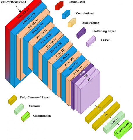
This work proposes a system for detecting several modulation schemes, commonly used within wireless communication systems based on a hybrid topology of CNN and LSTM networks as depicted in Figure 1. The system uses a spectrogram as its input format, which encodes the time and frequency resolution of the modulated signals. Here, we provide details of a system, its components, operating flow, and strengths.
Figure 1. Hybrid CNN-LSTM architecture for signal classification
3.1 Signal preprocessing
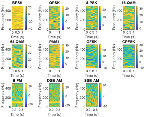
This system receives raw modulated signals as input. Examples of these include BPSK, QPSK, 8-PSK, 16-QAM, 64-QAM, PAM4, GFSK, CPFSK, B-FM, DSB-AM, and SSB-AM modulation schemes. The time-domain input signal is passed through the STFT to transform it in a time-frequency representation (in our case a spectrogram). STFT is a critical instrument for investigating the frequency richness of signals as they progress through time. Basically, it splits the input signal x(t) into overlapping chunks, which are mapped into the frequency domain using the Fourier transform. The signal preprocessing steps are as follows:
These preprocessing steps ensure that the spectrograms generated are detailed enough to capture the essential characteristics of the modulated signals while maintaining the computational efficiency required for model training.
Mathematical Formulation of STFT:
$X(t . f)=\int_{-\infty}^{\infty} x(\tau) h(t-\tau) e^{-j 2 \pi f \tau} d \tau$
where:
The STFT method splits the signal into small, overlapping windows, performs the Fourier Transform on each, and generates a 2D time-frequency diagram. In this diagram, time is represented on the x-axis, frequency on the y-axis, and the magnitude of the frequency is represented by color or intensity. By using spectrograms, the system effectively captures the key features of modulated signals in a format suitable for further analysis and classification.
3.2 CNNs
The CNN is a precise deep learning architecture used to process image data generally. CNNs have changed the game of computer vision by allowing machines to examine and classify images, identify objects, and even produce new images. Inspired by the human visual system, CNNs excel at identifying spatial hierarchies and complex image patterns.
A CNN consists of a complex arrangement of interconnected layers, each responsible for the extraction and transformation of features from input images. The convolutional layer is the first basic layer, where small filter matrices (kernels) are used to convolve with the input image. This detects local features such as edges, textures, and shapes, producing a feature map indicating important aspects of the image. By combining multiple filters, various features are captured, so the model is more capable of recognizing complex patterns. In CNNs, the equation for convolution is:
$Y_{i.j}=\sum_m \sum_n X_{i+m.j+n} \cdot W_{m.n}+b$ (1)
where:
The activation function is vital for improving the networks ability to learn complex representations. Their most common activation function is Rectifying Linear Unit (ReLU), which allows non-linearity while retaining important information about the input. ReLU is able to perform much faster, but only sacrifice the lower end of the data without sacrificing anything critical. Where the ReLU activation function is as such:
$\operatorname{ReLU}(x)=\max (0 . x)$ (2)
where:
After the convolution and activation stages, a pooling layer is applied to refine feature extraction by reducing the spatial dimensions of feature maps. This down-sampling process not only minimizes computational overhead but also enhances the model's robustness against slight variations in input images. The dominant pooling method is max pooling, which retains the most prominent feature by selecting the highest value within a defined region; for Max Pooling, the output is:
$Y_{i.j}=\max \left(X_{i.j} \cdot X_{i+1.j+1}.\ldots.X_{i+k.j+k}\right)$ (3)
where:
Table 1 presents the layer configuration of the CNN architecture. Each convolutional layer applies a kernel of size [3 × 3], which serves as a small filter that scans the input feature maps to detect local patterns such as edges and textures. The stride, set to [1 × 1] for convolutional layers, controls how far the kernel moves at each step, ensuring detailed feature extraction. In contrast, the max pooling layers use kernels of size [2 × 2] with a stride of [2 × 2] to downsample the feature maps, reducing spatial dimensions while retaining the most important features.
After extracting the data with 6 convolutional layers, it is then fed through a flattening layer: this turns the multidimensional data into one-dimensional data that can be processed by the LSTM and fully connected layers:
Flatten $(\mathrm{X})=$ Reshape $(\mathrm{X})$ (4)
Table 1. CNN layer configuration for hybrid CNN-LSTM architecture
|
Layer Type |
Dimensions |
Kernel Size |
Stride |
|
Input Layer |
(128 × 128 × 3) |
- |
- |
|
CNN Layer 1 |
(128 × 128 × 16) |
[3 × 3] |
[1 × 1] |
|
Max Pooling 1 |
(64 × 64 × 16) |
[2 × 2] |
[2 × 2] |
|
CNN Layer 2 |
(64 × 64 × 32) |
[3 × 3] |
[1 × 1] |
|
Max Pooling 2 |
(32 × 32 × 32) |
[2 × 2] |
[2 × 2] |
|
CNN Layer 3 |
(32 × 32 × 64) |
[3 × 3] |
[1 × 1] |
|
Max Pooling 3 |
(16 × 16 × 64) |
[2 × 2] |
[2 × 2] |
|
CNN Layer 4 |
(16 × 16 × 128) |
[3 × 3] |
[1 × 1] |
|
Max Pooling 4 |
(8 × 8 × 128) |
[2 × 2] |
[2 × 2] |
|
CNN Layer 5 |
(8 × 8 × 256) |
[3 × 3] |
[1 × 1] |
|
Max Pooling 5 |
(4 × 4 × 256) |
[2 × 2] |
[2 × 2] |
|
CNN Layer 6 |
(4 × 4 × 512) |
[3 × 3] |
[1 × 1] |
|
Max Pooling 6 |
(2 × 2 × 512) |
[2 × 2] |
[2 × 2] |
3.3 LSTM networks
LSTM networks are a specialized form of Recurrent Neural Networks (RNNs) that are designed to manage sequential data, particularly when long-term dependencies need to be captured. These networks excel in addressing the issue of the vanishing gradient, a challenge that causes traditional RNNs to fail at learning patterns over extended sequences. LSTM networks are built with three critical components: the input gate, which controls the information added to the memory; the forget gate, which regulates what data should be removed from the memory; and the output gate, which determines the information to be used as the output at each time step.
The forget gate in an LSTM network is responsible for deciding which parts of the memory (cell state) should be discarded, enabling the network to retain only the most relevant information for future processing.
The sigmoid activation outputs between 0 and 1 values, with 0 indicating full forget and 1 indicating full retention of data. By retaining only relevant historical data, this guarantees that only the information that is truly relevant has influence over the predictions. The equation for the forget gate is:
$f_t=\sigma\left(W_f\left[h_{t-1}.x_t\right]+b_f\right)$ (5)
where:
In flow: The input gate allows new information to flow into the cell state. The first one is an input gate layer that decides which information is going to be updated, along with a candidate value calculated with the tanh function to control the update. This enables the model to strike a balance between past accumulated knowledge and new information gained.
$i_t=\sigma\left(W_i\left[h_{t-1}.x_t\right]+b_i\right)$ (6)
where:
For the candidate memory cell, it is:
$\tilde{C}_t=\tanh \left(W_C\left[h_{t-1}.x_t\right]+b_C\right)$ (7)
where:
Finally, the output gate decides the information that is passed from the memory cell to the hidden state. It applies a sigmoid activation to decide how much cell state to output. This mechanism enables the model to transfer relevant information in a controlled manner, which significantly stabilizes long-distance connections. Therefore, LSTMs can better model complex correlational sequences more flexibly and better adapt to sequential tasks by estimating the time to remember or forget correlations. By playing the right amount of information to be stored/updated, LSTMs perform a lot better for long-term dependencies, as well as a lot of contextual information, than traditional RNNs.
$o_t=\sigma\left(W_o\left[h_{t-1}.x_t\right]+b_o\right)$ (8)
where:
After that, the cell state collects and updates information that is to be retained or discarded over time. It is updated at each time step using the forget gate and the input gate. The equation for the cell state is:
$C_t=f_t * C_{t-1}+i_t * \tilde{C}_t$ (9)
where:
The hidden state is the output of each step, which is either predicted or forwarded to the next step. It encodes the information of the sequence till the current time step.
Hidden state equation:
$h_t=o_t * \tanh \left(C_t\right)$ (10)
where:
After LSTM layers, 2 fully connected layers are used to combine the extracted features and learn complex representations for classification:
$z=W \cdot x+b$ (11)
where:
Finally, the output layer uses the Softmax function to convert the raw scores (logits) into probabilities for multi-class classification:
$P(y=i \mid \mathbf{x})=\frac{e^{z_i}}{\sum_j e^{z_j}}$ (12)
where:
Table 2 shows the LSTM layer configuration of the hybrid CNN-LSTM architecture. The first LSTM layer consists of 128 hidden units with a dropout rate of 0.2 to capture long-range dependencies in the data. The second LSTM layer, with 64 hidden units and the same dropout rate, adds further temporal context while helping to reduce overfitting.
Table 2. LSTM layer configuration for hybrid CNN-LSTM architecture
|
Layer Type |
Hidden Units |
Dropout |
Description |
|
LSTM Layer 1 |
128 |
0.2 |
First LSTM layer with 128 hidden units, captures long-range dependencies. |
|
LSTM Layer 2 |
64 |
0.2 |
Second LSTM layer with 64 hidden units, adds more temporal context. |
3.4 Hybrid CNN-LSTM model
This model takes advantage of the strengths of both CNNs and LSTMs. In addition, the use of spectrograms provides a powerful representation by converting signals into the time–frequency domain, allowing the model to extract both spectral and temporal features more efficiently. As illustrated in Figure 2, various modulation types are represented in the spectrograms, which further enhances the model’s ability to distinguish between different signal patterns.
Figure 2. Spectrogram of all modulation types
CNN Layer (6 Layers): Convolutional layers are used in a series to accept the spectrogram as input for extracting the spatial features. These layers identify patterns like edges, textures, and shapes in the spectrogram. Convolutional layers utilize filters to identify local patterns. Pooling layers (like max pooling): reduce the size of the feature maps.
LSTM Layer (2 Layers): Reshape the output of the CNN and input into 2 LSTM layers to learn temporal dependencies. LSTMs are very well adapted to dealing with data from sequences and able to capture long-range dependencies in the signal. The initial LSTM layer handles the input sequential data and captures relevant temporal features. The second LSTM layer adds more details to the time series feature representation and improves the accuracy of the modulation scheme classification. Fully Connected Layer: LSTM output is fed into fully connected layers to project the features onto the classes of modulation. Softmax Activation: The last layer applies a Softmax activation function that results in a probability distribution for the various modulation classes.
3.5 Workflow of the proposed system
Data Collection: Collect a dataset of modulated signals with known modulation types and various SNRs. And the data Generation in MATLAB with 2000 frames for eleven modulation types. Spectrogram Generation: Convert the raw signals to spectrograms via STFT. Data Splitting: Split the dataset into three sets:
4.1 Performance at different SNRs
(1) Low SNR (-20 dB):
At -20 dB, the model achieved an overall classification accuracy of 62.3%. This is a significant improvement compared to traditional methods, which typically fail to perform well under such noisy conditions.
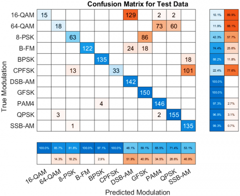
The confusion matrix (Figure 3) and Table 3 show that certain modulation types, such as DSB-AM, GFSK, PAM4, QPSK, and SSB-AM, were classified with high accuracy (ranging from 96.9% to 100%). However, other modulation types like 16-QAM and 64-QAM had lower accuracy (10.1% and 11.9%, respectively), indicating that these modulation schemes are more challenging to classify in extremely noisy environment is this work the hybrid CNN-LSTM model excels at low SNR due to the complementary strengths of CNNs and LSTMs. The CNN efficiently extracts spatial features even under high noise, while the LSTM mitigates noise by modeling temporal coherence, effectively filtering out irrelevant noise across time. This ability to model both spatial and temporal dependencies enables the hybrid model to maintain robust performance in noisy environments. We have validated this hypothesis with SNR-vs-feature visualizations, which show that while CNNs capture important spatial features even at low SNR, the LSTM layer ensures that these features remain coherent over time, contributing to improved classification performance. Table 4 presents the precision, recall, and F1-score of the hybrid CNN-LSTM model at an SNR of -20 dB for different modulation types. The results indicate how accurately the model can classify each modulation, with values closer to 1 representing better performance. Some modulation types, such as DSB-AM, GFSK, PAM4, QPSK, and SSB-AM, achieve perfect scores, while others like 16-QAM and 64-QAM show lower performance under this low SNR condition.
Figure 3. Confusion matrices of hybrid CNN-LSTM at signal-to-noise ratio = -20 dB
Table 3. The classification accuracy for all modulation types using hybrid CNN-LSTM at signal-to-noise ratio = -20 dB
|
Modulation Types |
SNR -20 dB |
|
16-QAM |
10.1% |
|
64-QAM |
11.9% |
|
8-PSK |
42.3% |
|
B-FM |
74.4% |
|
BPSK |
88.2% |
|
CPFSK |
22.4% |
|
DSB-AM |
100% |
|
GFSK |
100% |
|
PAM4 |
97.3% |
|
QPSK |
96.9% |
|
SSB-AM |
99.3% |
|
Accuracy |
62.3% |
Table 4. Precision, recall, and F1-score for hybrid CNN- LSTM at SNR = -20 dB
|
Modulation Type |
Precision |
Recall |
F1-Score |
|
16-QAM |
0.417 |
0.101 |
0.163 |
|
64-QAM |
0.199 |
0.399 |
0.265 |
|
8-PSK |
0.894 |
0.491 |
0.634 |
|
B-FM |
0.573 |
0.830 |
0.678 |
|
BPSK |
1.000 |
0.598 |
0.748 |
|
CPFSK |
0.584 |
1.000 |
0.738 |
|
DSB-AM |
1.000 |
1.000 |
1.000 |
|
GFSK |
1.000 |
1.000 |
1.000 |
|
PAM4 |
1.000 |
1.000 |
1.000 |
|
QPSK |
1.000 |
1.000 |
1.000 |
|
SSB-AM |
1.000 |
1.000 |
1.000 |
(2) Moderate SNR (0 dB):
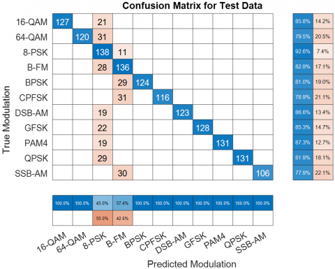
At 0 dB, the model's performance improved significantly, achieving an overall accuracy of 85.4%. The confusion matrix (Figure 4) and Table 5 show that most modulation types were classified with high accuracy, ranging from 77.9% to 92.6%.
Figure 4. Confusion matrices of hybrid CNN-LSTM at signal-to-noise ratio = 0 dB
Table 5. The classification accuracy for all modulation types using hybrid CNN-LSTM at signal-to-noise ratio = 0 dB
|
Modulation Types |
SNR 0 dB |
|
16-QAM |
85.8% |
|
64-QAM |
79.5% |
|
8-PSK |
92.6% |
|
B-FM |
82.9% |
|
BPSK |
81.0% |
|
CPFSK |
78.9% |
|
DSB-AM |
85.6% |
|
GFSK |
85.3% |
|
PAM4 |
87.3% |
|
QPSK |
81.9% |
|
SSB-AM |
77.9% |
|
Accuracy |
85.4% |
The results indicate that the model is capable of distinguishing between different modulation schemes more effectively as the SNR improves. However, some modulation types, such as CPFSK and SSB-AM, still posed challenges, with accuracies of 78.9% and 77.9%, respectively.
(3) High SNR (20 dB):
At 20 dB, the model achieved perfect classification accuracy (100%) across all modulation types, as shown in the confusion matrix (Figure 5) and Table 6. This demonstrates that the hybrid CNN-LSTM model is highly effective in high SNR conditions, where noise is minimal, and the signal is clear.
Table 7 shows the precision, recall, and F1-score of the hybrid CNN-LSTM model at an SNR of 20 dB for various modulation types. The results demonstrate that the model achieves perfect performance across all modulation types under this high SNR condition, with all metrics reaching 1.0, indicating excellent classification accuracy and reliability.
Figure 5. Confusion matrices of Hybrid CNN-LSTM at signal-to-noise ratio = 20 dB
Table 6. The classification accuracy for all modulation types using hybrid CNN-LSTM at signal-to-noise ratio = 20 dB
|
Modulation Types |
SNR 20 dB |
|
16-QAM |
100% |
|
64-QAM |
100% |
|
8-PSK |
100% |
|
B-FM |
100% |
|
BPSK |
100% |
|
CPFSK |
100% |
|
DSB-AM |
100% |
|
GFSK |
100% |
|
PAM4 |
100% |
|
QPSK |
100% |
|
SSB-AM |
100% |
|
Accuracy |
100% |
Table 7. Precision, recall, and F1-score for hybrid CNN-LSTM at SNR = 20 dB
|
Modulation |
Precision |
Recall |
F1-Score |
|
16-QAM |
1.0000 |
1.0000 |
1.0000 |
|
64-QAM |
1.0000 |
1.0000 |
1.0000 |
|
8-PSK |
1.0000 |
1.0000 |
1.0000 |
|
B-FM |
1.0000 |
1.0000 |
1.0000 |
|
BPSK |
1.0000 |
1.0000 |
1.0000 |
|
CPFSK |
1.0000 |
1.0000 |
1.0000 |
|
DSB-AM |
1.0000 |
1.0000 |
1.0000 |
|
GFSK |
1.0000 |
1.0000 |
1.0000 |
|
PAM4 |
1.0000 |
1.0000 |
1.0000 |
|
QPSK |
1.0000 |
1.0000 |
1.0000 |
|
SSB-AM |
1.0000 |
1.0000 |
1.0000 |
Figure 6. Impact of SNR on modulation classification accuracy
Figure 6 illustrates the relationship between SNR and classification accuracy for different modulation schemes, including 8-PSK, CPFSK, 16-QAM, 64-QAM, and B-FM. The x-axis represents the SNR in decibels (dB), while the y-axis denotes the classification accuracy in percentage, which reflects the effectiveness of modulation recognition under varying noise conditions. The results indicate that at highly negative SNR values, particularly around -20 dB, classification accuracy remains low across all modulation types, with most values starting below 20%. However, as SNR increases, accuracy gradually improves, suggesting that as noise diminishes, the recognition capability of the model becomes more reliable.
B-FM maintains relatively high classification accuracy even in low SNR conditions, demonstrating greater resilience to noise compared to the other modulation types. As the SNR approaches 0 dB, all modulation schemes exhibit a noticeable rise in accuracy, with CPFSK, 16-QAM, and 64-QAM showing substantial improvements. Beyond 0 dB, accuracy continues to increase, with most modulation types surpassing 80% accuracy at around 5 dB. This trend suggests that once the noise level is sufficiently reduced, the classifier can effectively distinguish between different modulation schemes.
At higher SNR values, particularly above 10 dB, all modulation types converge towards nearly perfect classification accuracy, reaching close to 100%. This indicates that under minimal noise interference, modulation recognition becomes highly reliable. Among the modulation types, 8-PSK exhibits the fastest rise in accuracy, indicating that it is more efficiently classified as noise decreases. In contrast, 16-QAM and 64-QAM, being higher-order modulations, struggle more at low SNR but experience rapid improvements as the SNR increases. These results across the board point to the effect of noise on modulation classification performance. Since analog modulations like B-FM are more resilient to noise impairment, while digital modulations (mainly QAM and PSK) are significantly more sensitive and demand larger SNR to provide reliable classification. The results are important as they can be used for signal recognition under different noise levels, which would significantly improve systems that are a practical part of day-to-day communication system design.
Table 8 presents the hyperparameter settings for a hybrid CNN-LSTM model under different SNR conditions. It includes the accuracy, epochs, learning rate, and mini-batch size used during training.
Table 8. Hyperparameter settings for the hybrid CNN-LSTM model
|
SNR (dB) |
Accuracy (%) |
Epochs |
Learning Rate |
Mini-Batch Size |
|
-20 |
62.3 |
1 |
0.001 |
32 |
|
0 |
85.4 |
1 |
0.001 |
32 |
|
20 |
100 |
1 |
0.001 |
64 |
4.2 Evaluation with different techniques
Traditional methods in the AMC field, engineers rely on feature extraction and statistical decision theory. However, these have problems in high noise environments. In contrast, our deep learning-based approach, particularly the CNN-LSTM architecture, is able to learn both spatial and temporal features of the signal: with this combined approach, it is much more robust across many different SNR ranges.
Our hybrid CNN-LSTM model consistently delivers superior classification accuracy (at 20 dB) compared to traditional methods, which typically achieve lower accuracy (for FFT + SVM at 20 dB). While the model requires GPU/TPU acceleration for efficient performance, its computational complexity is manageable with modern hardware, making it viable for real-time deployment in systems where high accuracy is essential.
Table 9 summarizes the accuracy achieved by previous researchers in this field using various CNN, LSTM, and hybrid architectures under different SNR conditions. While most studies report high accuracy values ranging from 91.8% to 99%, our proposed hybrid CNN-LSTM model demonstrates superior performance, especially under low SNR conditions, highlighting its robustness and effectiveness in accurately classifying diverse modulation types compared to earlier methods.
Table 9. The accuracy achieved by researchers in this field
|
Ref. |
Year |
Methodology |
SNR Range |
Accuracy |
|
[16] |
2023 |
Hybrid CNN-LSTM |
15 dB |
91.8% |
|
[19] |
2022 |
CNN-LSTM with Attention |
20 dB |
95.5% |
|
[20] |
2024 |
Gaussian-regularized CNN-LSTM |
10 dB |
96.4% |
|
[17] |
2023 |
Residual stack-aided CNN-LSTM |
15 dB |
93.7% |
|
[18] |
2021 |
Multidimensional CNN-LSTM |
18 dB |
93.2% |
|
[1] |
2020 |
Dual-stream CNN-LSTM |
10 dB |
92% |
|
[22] |
2021 |
CNN |
20 dB |
95% |
|
[10] |
2021 |
CNN |
20 dB |
97.2% |
|
[23] |
2022 |
CNN |
20 dB |
97.5% |
|
[24] |
2024 |
Bi LSTM |
20 dB |
99% |
|
[25] |
2018 |
DT |
20 dB |
98.5% |
|
[26] |
2016 |
HOC |
20 dB |
98% |
This study proposed a versatile method for AMC by combining a hybrid CNN-LSTM model based on a spectrogram representation of signals as features. Compared with traditional techniques that are frequently ineffective in low SNR scenarios, the proposed model results in obvious improvements in classification accuracy. The hybrid architecture successfully unites the spatial feature extraction power of CNNs and the temporal dependency apostate of LSTMs to guarantee stable modulation classification. These findings demonstrate the resilience of the proposed method, particularly in demanding noise environments, with the model successfully delivering a high level of accuracy across extensive SNR + noise spectrums, from -20 dB up to 20 dB. The proposed hybrid model based on CNN and LSTM outperforms traditional approaches while also demonstrating the promise of deep learning architectures to improve these systems' reliability and efficiency.
Future research may focus on optimizing the model for real-time applications in dynamic and low-SNR environments, incorporating advanced mechanisms like attention or transformers to further enhance feature extraction and classification precision. Ultimately, the findings underscore the transformative impact of deep learning techniques on AMC, offering valuable insights into future improvements for communication technologies under adverse conditions.
[1] Zhang, Z., Luo, H., Wang, C., Gan, C., Xiang, Y. (2020). Automatic modulation classification using CNN-LSTM based dual-stream structure. IEEE Transactions on Vehicular Technology, 69(11): 13521-13531. https://doi.org/10.1109/TVT.2020.3030018
[2] Liang, R., Yang, L., Wu, S., Li, H., Jiang, C. (2021). A three-stream CNN-LSTM network for automatic modulation classification. In 2021 13th International Conference on Wireless Communications and Signal Processing (WCSP), Changsha, China, pp. 1-5. https://doi.org/10.1109/WCSP52459.2021.9613477
[3] Wei, W., Mendel, J. M. (2000). Maximum-likelihood classification for digital amplitude-phase modulations. IEEE Transactions on Communications, 48(2): 189-193. https://doi.org/10.1109/26.823550
[4] Zhang, H., Nie, R., Lin, M., Wu, R., Xian, G., Gong, X., Yu, Q., Luo, R. (2021). A deep learning based algorithm with multi-level feature extraction for automatic modulation recognition. Wireless Networks, 27(7): 4665-4676. https://doi.org/10.1007/s11276-021-02758-0
[5] Essai, M.H., Atallah, H.A. (2023). Automatic modulation classification: Convolutional deep learning neural networks approaches. SVU-International Journal of Engineering Sciences and Applications, 4(1): 48-54. https://doi.org/10.21608/svusrc.2022.162662.1076
[6] Zuo, X., Yang, Y., Yao, R., Fan, Y., Li, L. (2024). An automatic modulation recognition algorithm based on time–frequency features and deep learning with fading channels. Remote Sensing, 16(23): 4550. https://doi.org/10.3390/rs16234550
[7] Ma, J., Hu, M., Wang, T., Yang, Z., Wan, L., Qiu, T. (2023). Automatic modulation classification in impulsive noise: Hyperbolic-tangent cyclic spectrum and multibranch attention shuffle network. IEEE Transactions on Instrumentation and Measurement, 72: 1-13. https://doi.org/10.1109/TIM.2023.3244798
[8] Zhou, L., Sun, Z., Wang, W. (2017). Learning to short-time Fourier transform in spectrum sensing. Physical Communication, 25: 420-425. https://doi.org/10.1016/j.phycom.2017.08.007
[9] Kojima, S., Maruta, K., Feng, Y., Ahn, C.J., Tarokh, V. (2021). CNN-based joint SNR and Doppler shift classification using spectrogram images for adaptive modulation and coding. IEEE Transactions on Communications, 69(8): 5152-5167. https://doi.org/10.1109/TCOMM.2021.3077565
[10] Huynh-The, T., Hua, C. H., Pham, Q.V., Kim, D.S. (2020). MCNet: An efficient CNN architecture for robust automatic modulation classification. IEEE Communications Letters, 24(4): 811-815. https://doi.org/10.1109/LCOMM.2020.2968030
[11] Venkata Subbarao, M., Samundiswary, P. (2021). Automatic modulation classification using cumulants and ensemble classifiers. In: Kalya, S., Kulkarni, M., Shivaprakasha, K.S. (eds) Advances in VLSI, Signal Processing, Power Electronics, IoT, Communication and Embedded Systems. Lecture Notes in Electrical Engineering, vol 752. Springer, Singapore. https://doi.org/10.1007/978-981-16-0443-0_9
[12] Cervantes, J., Garcia-Lamont, F., Rodríguez-Mazahua, L., Lopez, A. (2020). A comprehensive survey on support vector machine classification: Applications, challenges and trends. Neurocomputing, 408: 189-215. https://doi.org/10.1016/j.neucom.2019.10.118
[13] Elsagheer, M.M., Ramzy, S.M. (2023). A hybrid model for automatic modulation classification based on residual neural networks and long short term memory. Alexandria Engineering Journal, 67: 117-128. https://doi.org/10.1016/j.aej.2022.08.019
[14] Jia, H., Chen, N., Okada, M. (2021). Convolutional radio modulation recognition networks with attention models in wireless systems. ITE Technical Report, 45(24): 1-4.
[15] Le, H.K., Doan, V.S., Hoang, V.P. (2022). Ensemble of convolution neural networks for improving automatic modulation classification performance. Journal of Science and Technology, 20: 25-32. https://doi.org/10.31130/ud-jst.2022.293e
[16] Chakravarty, N., Dua, M., Dua, S. (2023). Automatic modulation classification using amalgam CNN-LSTM. In 2023 IEEE Radio and Antenna Days of the Indian Ocean (RADIO), Balaclava, Mauritius, pp. 1-2. https://doi.org/10.1109/RADIO58424.2023.10146088
[17] Kumar, A., Satija, U. (2023). Residual stack-aided hybrid CNN-LSTM-based automatic modulation classification for orthogonal time-frequency space system. IEEE Communications Letters, 27(12): 3255-3259. https://doi.org/10.1109/LCOMM.2023.3328011
[18] Wang, N., Liu, Y., Ma, L., Yang, Y., Wang, H. (2021). Multidimensional CNN-LSTM network for automatic modulation classification. Electronics, 10(14): 1649. https://doi.org/10.3390/electronics10141649
[19] Wang, Z., Wang, P., Lan, P. (2022). Automatic modulation classification based on CNN, LSTM and attention mechanism. In 2022 IEEE 8th International Conference on Computer and Communications (ICCC), Chengdu, China, pp. 105-110. https://doi.org/10.1109/ICCC56324.2022.10065667
[20] Elsagheer, M., Abd Elsayed, K., Ramzy, S. (2024). Optimizing automatic modulation classification through Gaussian-regularized hybrid CNN-LSTM architecture. JES. Journal of Engineering Sciences, 52(4): 46-61. https://doi.org/10.21608/jesaun.2024.271102.1315
[21] Li, Q., Zhou, X. (2023). LAANet: An efficient automatic modulation recognition model based on LSTM-Autoencoder and Attention Mechanism. In Advanced Data Mining and Applications. ADMA 2023. Lecture Notes in Computer Science, vol. 14177. Springer, Cham. https://doi.org/10.1007/978-3-031-46664-9_12
[22] Kaleem, Z., Ali, M., Ahmad, I., Khalid, W., Alkhayyat, A., Jamalipour, A. (2021). Artificial intelligence-driven real-time automatic modulation classification scheme for next-generation cellular networks. IEEE Access, 9: 155584-155597. https://doi.org/10.1109/ACCESS.2021.3128508
[23] Abdulkarem, A.M., Abedi, F., Ghanimi, H.M., Kumar, S., Al-Azzawi, W.K., Abbas, A.H., Abosinnee, A.S., Almaameri, I.M., Alkhayyat, A. (2022). Robust automatic modulation classification using convolutional deep neural network based on scalogram information. Computers, 11(11): 162. https://doi.org/10.3390/computers11110162
[24] Udaiwal, R., Baishya, N., Gupta, Y., Manoj, B.R. (2024). BiLSTM and attention-based modulation classification of realistic wireless signals. In 2024 International Conference on Signal Processing and Communications (SPCOM), Bangalore, India, pp. 1-5. https://doi.org/10.1109/SPCOM60851.2024.10631596
[25] Jiang, Y., Huang, S., Zhang, Y., Feng, Z., Zhang, D., Wu, C. (2018). Feature based modulation classification for overlapped signals. IEICE Transactions on Fundamentals of Electronics, Communications and Computer Sciences, 101(7): 1123-1126. https://doi.org/10.1587/transfun.E101.A.1123
[26] Abdelmutalab, A., Assaleh, K., El-Tarhuni, M. (2016). Automatic modulation classification based on high order cumulants and hierarchical polynomial classifiers. Physical Communication, 21: 10-18. https://doi.org/10.1016/j.phycom.2016.08.001