Diego O. Tenorio-Huarancca*![]() | Hemerson Lizarbe-Alarcon
| Hemerson Lizarbe-Alarcon![]() | Rocky G. Ayala-Bizarro
| Rocky G. Ayala-Bizarro![]() | Main G. Tenorio-Palomino
| Main G. Tenorio-Palomino![]() | Rualth G. Bravo-Anaya
| Rualth G. Bravo-Anaya![]() | Alex S. Ircañaupa-Huamaní
| Alex S. Ircañaupa-Huamaní![]() | Edward León-Palacios
| Edward León-Palacios![]() | Victor Bellido-Aedo
| Victor Bellido-Aedo![]()
© 2025 The authors. This article is published by IIETA and is licensed under the CC BY 4.0 license (http://creativecommons.org/licenses/by/4.0/).
OPEN ACCESS
Historic urban centers present a paradigmatic challenge in modern traffic management, characterized by narrow streets originally conceived for carriage and pedestrian circulation. This infrastructural incompatibility generates critical congestion, exacerbated in developing countries where fixed-time traffic signal systems predominate, lacking adaptive capacity and generating substantial inefficiencies of temporal, energy, and fuel resources. We developed a convolutional neural network model based on a customized You Only Look Once version 8 architecture for vehicle detection and classification. The model implements advanced temporal filtering to reduce false positives, vehicle tracking for unique counting, and a comprehensive 13-stage traffic signal optimization algorithm that correlates detected vehicular density with cycle times. The system maintains operational robustness under adverse conditions, including precipitation, cloudiness, shadows cast by colonial mansions, vehicular occlusion phenomena, and luminous glare. Implementation was evaluated through video recordings from the Historic Center of Ayacucho, using strategically positioned cameras to determine vehicular density at various time periods. The model, trained for 126 epochs with Early Stopping on 3,000 images, achieves 88.7% precision, recall of 0.832/0.834 (validation/evaluation), establishing a robust solution for urban heritage contexts.
complex scenarios, convolutional neural networks, historic centers, intelligent traffic lights, traffic congestion, You Only Look Once
In the city of Ayacucho, vehicular congestion emerges as one of the principal challenges confronting public authorities. This situation is aggravated by the historic nature of its center, a colonial city whose original layout was not conceived for motorized vehicle transit, but primarily for the movement of carriages and pedestrians. Additionally, Ayacucho presents a monocentric structure where most commercial, educational, and labor activities converge toward the city center. This centralization causes the narrow streets of the historic center to hinder optimal integration of vehicular flow with the main arterial and secondary roads to which these streets converge. During peak hours, these narrow thoroughfares prove insufficient to absorb vehicular demand. This limitation obstructs the implementation of an efficient traffic regulation system, manifesting in congested transit characterized by slow circulation.
As an aggravating factor, vehicular traffic control in Ayacucho is conducted through fixed-time traffic signals that operate independently and in isolation, with pre-established cycles that do not respond to actual vehicular demand. Traffic controlled by fixed time intervals is one of the leading causes of traffic jams [1]. These fixed times are susceptible to rapid deprogramming, generating “red wave” patterns that, far from facilitating circulation, significantly obstruct vehicular flow. Vehicular congestion in historic centers constitutes one of the most complex challenges of contemporary urban mobility, characterized by inherent structural limitations.
The Ayacucho population daily experiences significant loss of productive time when trapped in traffic. A study showed that every year, drivers in the UK waste more than a day in traffic jams [2]. According to a survey, people waste 8.15 million hours yearly in traffic jams [3]. Meanwhile, in Peru the loss reached 27,000 million soles in 2017 [4]. This time loss not only implies a decrease in society’s general productivity, caused by the loss of valuable work hours, but also translates into tangible economic losses. Additionally, vehicular congestion causes a significant increase in stress for both citizens and drivers moving through the city. These effects are compounded by increased fuel consumption, directly proportional to the increase in constant vehicle stops and starts. Traffic congestion also aggravates the environmental pollution problem by increasing fuel consumption rate due to increased vehicle stops and restarts [5].
Finally, and crucially, vehicular congestion contributes to environmental quality degradation and increased noise pollution, generating health problems that affect the entire Ayacucho population. Congestion in traffic systems leads to significant environmental issues, including air pollution, greenhouse gas emissions, and adverse effects on living conditions. Vehicles release pollutants like carbon monoxide, nitrogen oxides, and particulates, resulting in noise pollution and higher travel expenses [6]. It is precisely this complex situation that drives the present proposal and motivates the search for a solution.
With the purpose of addressing vehicular congestion issues, we develop a traffic signal automation system based on YOLOv8 that overcomes the inherent limitations of fixed-time traffic signals responsible for current congestion problems. Through real-time video transmissions from cameras strategically positioned to maximize coverage and eliminate blind spots, this tool is conceived as an effective means to mitigate vehicular congestion in Ayacucho’s historic city center. The vehicular traffic model demonstrates its efficacy against vehicular flow variability fluctuations, operating optimally under diverse environmental conditions such as precipitation (a representative phenomenon in Ayacucho between December and March), sunny periods, cloudiness, shadows caused by colonial mansions, and nighttime environments where glare phenomena occur, thereby addressing critical traffic scenarios in heritage areas with unique urban characteristics. The proposed adaptive system generates timing cycles based on real-time PCU density analysis, contrasting with traditional fixed-time systems that operate with predetermined cycles independent of actual vehicular demand.
2.1 Vehicle detection architectures in complex environments
Recent advances in computer vision have enabled the development of robust vehicle detection systems capable of operating under diverse environmental conditions. Prayitno et al. [7] demonstrated how distributed sensing architectures with cooperative observers can enhance detection reliability in vehicle platoons by sharing state information across vehicles, providing redundancy and improved estimation accuracy in challenging environmental conditions. Wang et al. [8] developed RAGENet, a controlled fusion architecture integrating foggy image processing through YOLOv8, achieving superior performance metrics. However, their framework remains limited to congestion recognition without considering subsequent traffic signal optimization.
Research on meteorological robustness has explored enhancement techniques for adverse conditions. Kiran et al. [9] implemented YOLOv4 improvements through Retinex Multi-scale techniques and Pulse-Coupled Neural Networks, surpassing existing methods under variable climatic scenarios. Xu et al. [10] introduced YOLO-HyperVision by integrating Vision Transformers into YOLOv5 for aerial detection, improving mean average precision in images where objects exhibit significant scale differences.
Comparative analysis of YOLO architectures conducted by Lin and Lee [11] revealed performance variations among versions (v5-v8) under identical conditions, complementing public datasets with real vehicular camera images. Nevertheless, these approaches target autonomous vehicle applications without addressing urban traffic management.
2.2 Adaptive traffic signal control systems
Dynamic signal control has emerged as a promising alternative to traditional fixed-timing systems. Macherla et al. [12] demonstrated that deep reinforcement learning combined with recurrent neural networks can effectively optimize traffic signal control in 5G-enabled Internet of Vehicles environments, achieving superior performance in reducing waiting times by incorporating real-time vehicle interactions and network state information into adaptive signal timing decisions. Duc et al. [13] implemented YOLOv8-based density analysis for automatic traffic signal timing adjustment, achieving notable detection precision but limiting applicability to conventional urban intersections. Naithani and Jain [14] proposed conceptual frameworks incorporating emergency vehicle detection through RF technology, though practical validation remains pending.
Abbas et al. [1] developed real-time vehicle density-based algorithms using Faster R-CNN, demonstrating high classification and detection precision under different lighting conditions in developing country contexts. Saseendran et al. [15] introduced automatic systems utilizing live images for vehicle type detection and density calculation through image processing and artificial intelligence.
Rashad and Ali [16] explored cost-effective monitoring systems using Android-based smart units with YOLOv8 enhanced through SAHI algorithms for small and distant objects. However, these systems lack specific considerations for historic centers and heterogeneous local vehicle fleet characteristics.
2.3 Vehicle tracking and counting integration
Comprehensive traffic management requires advanced tracking and precise counting capabilities. Pudaruth et al. [17] synthesized solutions based on deep neural networks to detect, track, and count different vehicle types in real-time, achieving 96.1% average counting precision and 94.4% classification accuracy. Li and Lv [18] proposed tracking methods based on YOLO and residual networks, introducing attention mechanisms and decoupled head strategies.
Bui et al. [19] combined improved YOLOv5s with optimized DeepSORT algorithms, introducing AIFI modules and optimizing Kalman filters for more precise vehicle state predictions. Azimjonov et al. [20] developed systems whose traffic flow extraction processes raw camera images through detection and tracking algorithms, outperforming Kalman filter-based trackers in counting accuracy.
Rasheed et al. [21] implemented YOLOv2 principles for real-time vehicle detection and counting, providing robust object positioning functionality and high frames per second. Nevertheless, these approaches primarily focus on highway environments rather than complex urban intersections.
2.4 Machine learning-based optimization
Optimization approaches have incorporated advanced machine learning techniques for vehicular flow enhancement. Patil et al. [22] presented systems leveraging machine learning and computer vision to monitor vehicle density and optimize traffic light timing, employing real-time detection through deep convolutional networks. Kunekar et al. [23] combined computer vision and machine learning to simulate complex incoming traffic at signalized intersections.
Pujari and Kumar [24] employed computer vision and machine learning to identify opposing traffic flow characteristics at signalized intersections. Lavanya et al. [25] combined YOLO with Kafka architecture to create traffic density evaluation methods in real-time scenarios, predicting vehicular density through live streaming data collection.
Ottom and Al-Omari [26] proposed adaptive systems for determining vehicle types and calculating intersection numbers using pattern detection methods, comparing R-CNN, Fast R-CNN, Faster R-CNN, SSD, and YOLOv4 algorithms, determining that YOLOv4 achieved highest vehicle identification with 86.4% mAP.
2.5 Specialized applications and case studies
Recent investigations have explored specialized applications in specific contexts. Salekin et al. [27] presented vehicle classification using YOLOv8 transfer learning models customized for Bangladeshi native vehicles, achieving high 91.3% mAP. Hendrawan et al. [28] proposed intelligent monitoring systems based on real-time artificial analysis of YOLO, incorporating C3X modules in the YOLO backbone to enhance feature extraction capabilities.
Arafat et al. [29] developed cost-effective AI-based systems for vehicle detection and traffic monitoring, implementing models on Raspberry Pi to achieve simple and affordable solutions. Anwar et al. [30] proposed intelligent management by measuring vehicular traffic density through real-time detection and image processing.
Jain et al. [31] conducted comparative performance analysis of YOLO algorithms and their evolved versions (v1-v4) for real-time traffic scenarios, employing SORT algorithms for efficient tracking. However, these implementations generally lack validation in heritage environments with specific architectural constraints.
3.1 Dataset collection
3.1.1 Camera installation in Ayacucho Historic Center
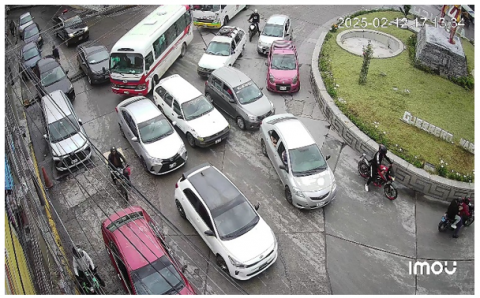
We implemented the installation of two surveillance cameras strategically positioned at the top of light poles to maximize coverage and eliminate blind spots. Figure 1 and Figure 2 show the frontal and inclined camera perspectives, respectively, capturing the traffic flow in the historic center. Additionally, an internet system was implemented to enable real-time vehicle monitoring. A rigid support arm was designed to ensure stability and secure camera mounting. Stability and proper fixation are fundamental for acquiring sharp and reliable images, even under adverse weather conditions. This stability not only ensures the visual quality of captured data but also enables precise adjustment of focus and camera angles, guaranteeing the acquisition of accurate and relevant vehicular information for traffic analysis. A specialized crane truck was employed to reach the desired heights and locations, elevating and positioning the video surveillance equipment, thus ensuring efficient and safe installation of the devices.
Figure 1. Traffic congestion: Camera 01-Frontal view
Figure 2. Traffic congestion: Camera 02-Inclined view
3.1.2 Focus, quality, and camera angle configuration
Once both cameras were installed, the Imou Life application was utilized to configure their optimal operation. Focus was adjusted to obtain sharp images, desired video quality was selected, and each camera’s angle was oriented to cover areas of interest. This fine-tuning process ensured effective surveillance of the monitored areas.
3.1.3 Data collection strategy
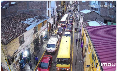
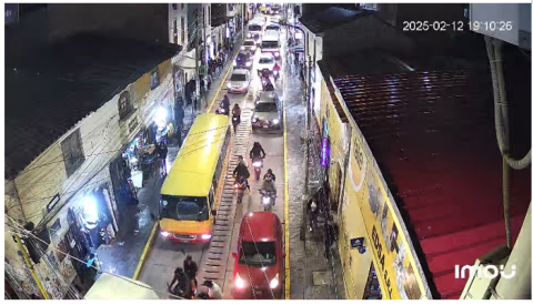
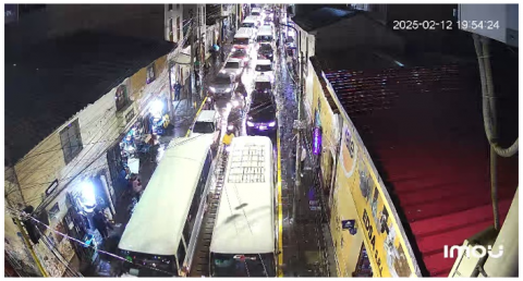
Images were captured under diverse traffic conditions during peak hours (7:30–8:30 AM, 1:00–2:30 PM, 6:30–8:00 PM), while also collecting a significant amount of data during periods of lower vehicular congestion. Furthermore, images were captured under various lighting conditions, including sunny days, rainy weather, sunsets, nighttime scenes where vehicle high beams create glare phenomena, and shadow scenes caused by colonial buildings. Figures 3-8 illustrate representative samples of image captures under different environmental conditions: sunny conditions (Figure 3), shadow conditions caused by colonial structures (Figure 4), cloudy conditions (Figure 5), sunset scenarios (Figure 6), nighttime conditions (Figure 7), and precipitation conditions (Figure 8). This diverse variety of data is fundamental for training the model to identify objects reliably and accurately, regardless of the lighting conditions present. This diverse variety of data is fundamental for training the model to identify objects reliably and accurately, regardless of the lighting conditions present.
Figure 3. Image capture under sunny conditions
Figure 4. Image capture under shadow conditions caused by colonial structures
Figure 5. Image capture under cloudy conditions
Figure 6. Image capture during sunset scenarios
Figure 7. Image capture under nighttime conditions
Figure 8. Image capture under precipitation conditions
A total of 3,000 local images in JPG format were captured from cameras 01 and 02, covering diverse lighting and weather conditions (day, night, rain, sun, temporal variability). This variety is crucial for developing a highly robust model even in challenging situations, avoiding dependence solely on ideal conditions.
Eight vehicle categories (classes) were defined as shown in Table 1:
Table 1. Definition of class number and dataset distribution by vehicle class
|
Class |
Description |
Approximate Instances |
|
A M MB PU MT
CP RC CG |
Cars/Station Wagons Motorcycles/ Bicycles Microbuses Pick-ups/SUVs Motorcycles Taxis/ Cargo Motorcycles Small Trucks C2/C3 Rural Combis/Panels Large Trucks C4/8 × 4 |
15,000 12,500 4,400 1,800 1,000
500 500 500 |
3.1.4 Ethical considerations and regulatory compliance
Video data collection in Ayacucho's heritage district was conducted following comprehensive regulatory protocols and ethical research standards. The installation of surveillance cameras required formal approval from multiple municipal departments of the Provincial Municipality of Huamanga, including Transit and Road Safety Sub-management, Citizen Security Sub-management, and the Information and Communications Technology Unit (UTIC).
The municipal technical evaluation confirmed equipment specifications, installation safety protocols, and regulatory compliance for public space monitoring. All installations followed municipal guidelines for camera positioning, avoiding obstruction of existing infrastructure and ensuring public safety during setup operations.
Data management protocols ensure strict privacy protection through a sworn declaration (declaración jurada) establishing exclusive researcher access to raw video data solely for research purposes. All data undergoes automatic anonymization of identifiable elements including vehicle license plates and pedestrian faces before analysis. Video retention is limited to the research duration with systematic deletion upon project completion, following institutional data protection guidelines.
The study complies with Peruvian data protection regulations and maintains full transparency with municipal authorities regarding research objectives, data handling procedures, and exclusive researcher custody of sensitive materials. Access to processed anonymized datasets is available for academic validation upon request, while raw video data remains under exclusive researcher control as per municipal authorization requirements.
3.2 Labelme annotation
Annotation was performed using Labelme software with the Segment Anything (Speed) tool for assisted segmentation. This approach enables precise vehicle boundary delineation even in high congestion scenarios where vehicles are in close proximity. The segmentation masks generated by SAM within Labelme were subsequently converted from JSON format to YOLO detection format for model training.
3.3 Model training
3.3.1 JSON to YOLO format conversion
Following the acquisition of 3,000 annotation files in JSON format, conversion to YOLO format was per formed. To effectively train the YOLO model and evaluate its generalization capability, the dataset was divided into a 70% proportion for training (2,100 images) and 30% (900 images) for validation.
3.3.2 126-Epoch training
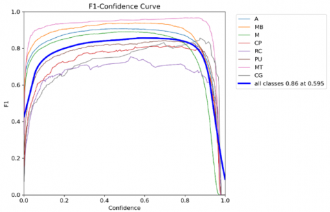
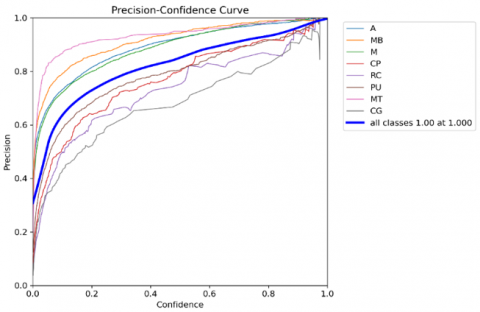
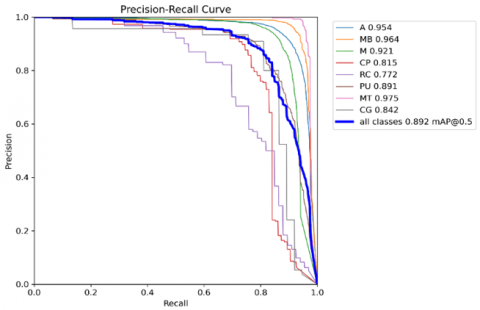
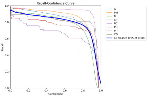
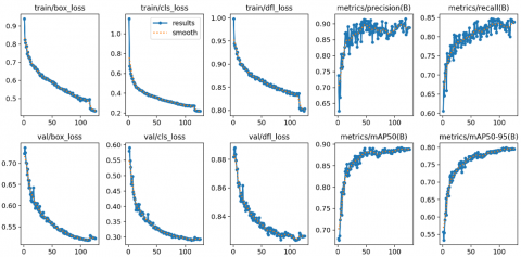
YOLOv8m (medium) was selected for training due to its superior benefits in vehicle detection and classification. The training process was conducted with various epoch configurations: 1, 20, 50, 100, 126, and 150 epochs, seeking to prevent overfitting. Complete results are shown for 126 epochs. The selection of 126 epochs as a key point is based on early stopping intervention, which indicated the optimal moment to halt training. The training performance is visualized through multiple evaluation curves: Figure 9 shows the F1-confidence curve, Figure 10 presents the precision-confidence curve, Figure 11 displays the precision-recall curve, Figure 12 illustrates the recall-confidence curve, and Figure 13 shows the comprehensive training and validation metrics across all 126 epochs. These curves demonstrate the model's learning progression and convergence behavior throughout the training process.
Figure 9. F1-confidence curve
Figure 10. Precision-confidence curve
Figure 11. Precision-recall curve
Figure 12. Recall-confidence curve
Figure 13. Training and validation metrics-126 epochs
3.4 Vehicle detection, classification, and counting description
The system implements a comprehensive multi-stage pipeline for vehicle detection, classification, and counting specifically optimized for heritage urban environments. The framework processes video streams using YOLOv8 as a specialized convolutional neural network for detection and classification, integrating advanced temporal filtering to eliminate false positives and an intelligent tracking algorithm that assigns unique identifiers to each vehicle based on spatial proximity and detection confidence. This robust architecture operates through six sequential stages that ensure optimal performance under adverse conditions typical of historic city centers, including colonial architecture shadows, narrow street configurations, and variable lighting scenarios.
3.4.1 YOLOV8 inference engine
The detection module utilizes YOLOv8 medium architecture as the core inference engine with the following configuration parameters: input resolution 640 × 640 pixels, confidence threshold 0.6, NMS IoU threshold 0.5, and multi-scale detection at 3 scales (8 ×, 16 ×, 32 × downsampling). The model performs initial object detection through:
3.4.2 Proposal decoding and coordinate transformation
The detection head outputs require coordinate transformation from relative to absolute positions:
$x=\left(\sigma\left(t_x\right)+c_x\right) \times$ stride (1)
$y=\left(\sigma\left(t_y\right)+c_y\right) \times$ stride (2)
$w=p_w \times e^{t_w}, h=p_h \times e^{t_h}$ (3)
where,
- tx, ty, tw, th = predicted offsets from YOLO head
- cx, cy = grid cell coordinates
- σ = sigmoid activation function
- pw, ph = anchor box dimensions
- stride = downsampling factor (8, 16, 32 for YOLOv8)
3.4.3 Static filtering and non-maximum suppression
Initial filtering removes low-confidence detections and overlapping proposals using the following parameters:
3.4.4 Temporal filtering for false positive reduction
Advanced temporal consistency checking addresses environmental artifacts common in heritage urban settings:
3.4.5 Intelligent vehicle tracking and unique identification
Sophisticated tracking algorithm assigns persistent identifiers to vehicles across frames:
$\sqrt{\left(x_c-x_c^{\prime}\right)^2+\left(y_c-y_c^{\prime}\right)^2}<50$ (4)
pixels, assign existing ID; otherwise, create new identifier.
3.4.6 Vehicle tracking methodology
Vehicle tracking employs centroid-based proximity matching with a 50-pixel threshold for vehicle association across frames. This threshold was selected as a practical compromise between maintaining tracking continuity and avoiding false associations in the specific resolution and traffic density conditions of the study. The centroid-based approach calculates the geometric center of each detected bounding box and associates vehicles across consecutive frames when the distance between centroids falls below the established threshold.
While more sophisticated tracking algorithms such as DeepSORT or Hungarian assignment with IoU matching could potentially improve performance, the centroid-based approach provides adequate tracking accuracy for traffic density analysis purposes while maintaining computational efficiency required for real-time operation. This methodology proves particularly effective in heritage urban environments where camera positions are fixed and vehicle movement patterns are relatively predictable within the constrained geometric layout of historic intersections.
The simplicity of the tracking algorithm also contributes to system robustness under the challenging visual conditions typical of colonial urban centers, including variable lighting, architectural shadows, and weather-related visibility changes, where more complex tracking methods might be susceptible to feature extraction failures.
3.4.7 PCU-based traffic analysis
Final stage converts heterogeneous vehicle counts into standardized traffic units:
$P C U_{(t)}=\sum_{v \in V_t} u_{c(v)}$ (5)
where, Vt is the set of unique IDs detected at time t.
This integrated approach addresses the unique challenges of heritage urban environments while maintaining computational efficiency required for real-time traffic management applications.
3.5 Comprehensive traffic signal optimization algorithm
The developed traffic signal optimization algorithm combines vehicular detection via YOLOv8 with consolidated traffic engineering principles and driver psychology fundamentals, implementing an adaptive approach based on contextualized PCU density of the vehicular fleet in Ayacucho’s historic center. The PCU (Passenger Car Unit) values assigned to each vehicle class are presented in Table 2. These values reflect the relative impact of each vehicle class on traffic flow and road capacity, derived from the Sustainable Urban Mobility Plan of Huamanga.
Table 2. PCU values for the 8 vehicle classes
|
Class |
Description |
PCU |
|
A M MB PU MT
CP RC CG |
Cars/Station Wagons Motorcycles/ Bicycles Microbuses Pick-ups/SUVs Motorcycles Taxis/ Cargo Motorcycles Small Trucks C2/C3 Rural Combis/Panels Large Trucks C4/8 × 4 |
1.00 0.33 2.50 1.25 0.75
2.50 2.00 3.50 |
The Passenger Car Unit (PCU) is a standardized metric in transportation engineering that establishes relative values for different vehicle types according to their impact on vehicular flow and road capacity, enabling traffic analysis homogenization by converting heterogeneous vehicular composition into comparable equivalent units. The model proposed in this study implements specific PCU values that have been adapted to reflect local conditions of the study area.
The developed algorithm constitutes a comprehensive 13-stage traffic signal optimization system that represents a significant scientific innovation by combining vehicular detection via YOLOv8 with consolidated traffic engineering principles and driver psychology fundamentals.
3.5.1 Mathematical formulation of the algorithm
From an observation interval Tobs (e.g., 45 seconds), the algorithm processes the following stages.
a. Vehicular composition and total PCU calculation
The vehicular counting system is based on multiple object detection and tracking, implementing advanced temporal filtering to avoid counting duplicates. The weighted sum according to specific PCU values enables normalization of vehicular heterogeneity to comparable standards.
For each vehicular class i detected during the observation period, the calculation is:
$P C U_{ {total }}=\sum_{i=1}^n N_i x P C U_i$ (6)
where:
b. PCU density calculation
The PCU density is maintained in PCU/s units for direct application in traffic signal optimization calculations, providing immediate responsiveness to vehicular demand fluctuations.
$\rho=\frac{P C U_{ {total }}}{T_{{obs }}}(\mathrm{PCU} / \mathrm{s})$ (7)
3.5.2 Saturation degree determination
This is based on calibration studies by the study [32] that establish 1,900 PCU/hour/lane as ideal capacity for optimal geometric conditions (3.6 m lane, considerable grade, good pavement—characteristics of Ayacucho’s historic center). The relationship between delay and saturation degree follows an exponential, non-linear curve, requiring specific adjustments.
Ideal capacity per second is defined as:
$C=\frac{1900}{3600}=0.528 P C U / s / lane$ (8)
Saturation degree is calculated as:
$\gamma=min \left(1.0, \frac{\rho}{c}\right)=min \left(1.0, \frac{\rho}{0.528}\right)$ (9)
3.5.3 Level of service evaluation
Evaluation is performed through an adaptation of the study [31], adjusted to local context particularities. This classification directly correlates PCU density ranges with driver psychological states, from comfort to severe stress.
Level of service is determined according to standard density:
$\text {Level of Service} =\left\{\begin{array}{cc}\text { A (Free flow), } & \rho_{s t d}<9 \\ \text { B (Reasonably stable flow), } & 9 \leq \rho_{s t d}<14 \\ \text { C (Stable flow), } & 14 \leq \rho_{s t d}<19 \\ \text { D (Flow approaching unstable), } & 19 \leq \rho_{s t d}<24 \\ \text { E (Unstable flow), } & 24 \leq \rho_{s t d}<29 \\ \text { F (Congested flow), } & \rho_{s t d} \geq 29 \end{array}\right.$ (10)
3.5.4 Parameter calibration methodology
The scaling factors and increment coefficients implemented in this algorithm combine established traffic engineering principles with empirical calibration using the 32-scenario dataset. The proportional increment factors (Eq. (12)) derive from Webster's compensation theory [33], with exponents (0.75, 0.65) adjusted through iterative analysis of the video data to optimize performance across varying saturation levels. The scale factor threshold of 25 PCU (Eq. (14)) was determined through statistical analysis of the dataset's PCU distribution, representing the median demand level that triggers proportional scaling. Dynamic increment percentages (Eq. (15)) were calibrated by correlating density patterns observed in the historic center with required timing adjustments, validated across the complete 32-video evaluation set.
While these parameters demonstrate effectiveness across the evaluated scenarios, further calibration with expanded datasets from diverse traffic conditions and geometric configurations could enhance the algorithm's generalizability and optimize performance for broader applications in heritage urban environments.
3.5.5 Variable base green time
Based on the study conducted by Kell and Fullerton [34] from the Institute of Transportation Engineers (ITE) and driver psychology studies [35], a minimum phase time of 7 seconds is required, but psychological evidence demonstrates that green times less than 15 seconds generate frustration and increase traffic signal violations.
A variable minimum green time is established considering total PCU demand and driver psychology principles:
$t_{v, { base }}=\left\{\begin{array}{cc}18 \mathrm{~s}, & \sum P C U>20 \\ 16 \mathrm{~s}, & 10<\sum P C U \leq 20 \\ 15 \mathrm{~s}, & \sum P C U \leq 10\end{array}\right.$ (11)
3.5.6 Proportional increment (Adapted Webster)
This is based on compensation principles by Brosseau et al. [36], who mathematically demonstrated that intersections with highly saturated approaches require proportionally greater time allocations. Additional increment is calculated exclusively based on saturation degree, adapting to specific local traffic conditions.
$A=\left\{\begin{array}{lc}3.0 \gamma^{0.75}, & \gamma>0.7 \\ 2.8 \gamma^{0.65}, & \text { other cases }\end{array}\right.$ (12)
For low saturation conditions $(\gamma<0.15)$, a linear interpolation factor is applied:
$A=w_l(4.5 \gamma)+\left(1-w_l\right) A, w_l=\frac{0.15-\gamma}{0.15}$ (13)
3.5.7 Scale factor by total demand
Based on microsimulation studies that confirmed additional scale factors, beyond saturation degree, are necessary to optimize intersection operation with high total traffic volume. This factor explicitly recognizes that intersections with greater demand require proportionally longer cycles.
A multiplier factor is applied based directly on total PCU demand:
$S=\operatorname{clamp}\left(\frac{\Sigma P C U}{25}, 1.0,1.2\right)$ (14)
where, clamp(x,a,b) = max(a,min(x,b)).
3.5.8 Dynamic additional increment
This increment derives from empirical observation showing particular traffic patterns in the study area (Historic center of Ayacucho city), where passenger pickup activity generates specific behaviors that justify additional adjustments proportional to vehicular density.
$I=\left\{\begin{array}{cc}1+0.25 \gamma, & \gamma>0.8 \\ 1+0.20 \gamma, & \gamma>0.5 \\ 1+0.18 \gamma, & \text { other cases }\end{array}\right.$ (15)
3.5.9 Optimized green time calculation
The 60-second restriction as maximum green time is based on research by Webster [33] demonstrating that green times exceeding 60 seconds generate excessive delays at secondary approaches and impatient behavior in pedestrians.
Optimized green time is calculated by integrating all adjustment factors:
$t_{v, { opt }}=min \left(t_{v, { base }}+(4.0 \times A \times S \times I), 60\right)$ (16)
where, each factor contributes proportionally to the increment over base time.
3.5.10 Adaptive amber time calculation
The dilemma zone concept associated with amber light is widely recognized as a critical area where vehicles can neither stop safely nor traverse the intersection during the amber interval [37]. The calculation considers driver perception-reaction time (1-1.5 seconds), approach speed, and safe braking distance.
Amber time is adjusted according to traffic density, considering driver perception-reaction time and dilemma zone:
$t_a=\operatorname{clamp}(3+1.2 \sqrt{\gamma}, 3,5)$ (17)
3.5.11 Total cycle determination
All-red time is a safety measure that allows vehicles that entered during amber to completely finish crossing before perpendicular traffic begins moving, reducing the risk of lateral “T-bone” type accidents.
For the main traffic signal (Signal 1 - Camera 1 detection):
$\text{Green Phase}_1=t_{v, { opt }}\left(P C U_1\right)$ (18)
$\text{Amber Phase}_1=t_a\left(\rho_1\right)$ (19)
For the perpendicular traffic signal (Signal 2 - Camera 2 detection):
$t_{{red }, 2}=t_{v, { opt }}\left(P C U_1\right)+t_a\left(\rho_1\right)+1.0$ (20)
$\text{Green Phase}_2=t_{v, { opt }}\left(P C U_2\right)$ (21)
$\text{Amber Phase}_2=t_a\left(\rho_2\right)$ (22)
Total cycle is defined as:
$\begin{gathered}\text { Total Cycle }=t_{v, { opt }}\left(P C U_1\right)+t_a\left(\rho_1\right)+ t_{v, { opt }}\left(P C U_2\right)+t_a\left(\rho_2\right)+2.0\end{gathered}$ (23)
3.5.12 Export and visualizations
CSV: detailed counting, PCU, and traffic signal timing data.
Graphics:
3.5.13 Complete algorithm summary
The system processes the following input and output variables:
Input variables:
Output variables:
3.6 Image pre-processing
To homogenize lighting conditions and focus attention on the roadway, each raw frame undergoes:
ROI Cropping
Aspect-preserving resizing
$s=min \left(\frac{N}{\omega}, \frac{N}{h}\right)$ (24)
Non-linear Contrast Equalization
$\psi(c)=4 c-6 c^2+4 c^3-c^4, c=Y(i, j)$ (25)
This block reduces luminance and spatial variability, improving detection under adverse conditions (back-lighting, colonial building shadows, rain).
3.7 Data management in Colab-drive
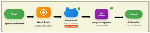
Figure 14 illustrates the complete data transmission workflow of the proposed intelligent traffic light system. The process begins with system activation, followed by video input capture from traffic intersections. Data is processed through Google Colab using YOLOv8 algorithms with cloud computing capabilities. The integrated algorithm performs temporal filtering and analysis to generate optimized traffic light timing calculations as the final output.
Figure 14. Data transmission flow in our proposed framework
3.8 Detection and feature extraction
The network is structured into four blocks:
Backbone (Focus → CSP → SPPF)
Neck (PAFPN)
Detection Head: At each scale, predicts for each cell and anchor: offsets (tx,ty,tw,th), objectness pobj, and class probabilities pc.
Decoding:
$x=\left(\sigma\left(t_x\right)+c_x\right) \times$ stride (26)
$w=p_w \times exp \left(t_w\right)$ (27)
$y=\left(\sigma\left(t_y\right)+c_y\right) \times$ stride (28)
$h=p_h \times exp \left(t_h\right)$ (29)
Training hyperparameters:
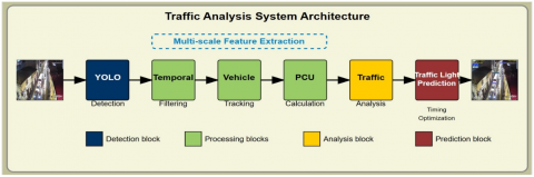
Figure 15 presents the comprehensive architecture of the proposed traffic analysis system, showing the sequential pipeline from video input to traffic signal optimization. The system initiates with YOLO detection (blue block) for real-time vehicle identification, followed by temporal filtering (green block) that eliminates false positives and assigns unique identifiers for accurate counting. The PCU calculation block (green block) converts heterogeneous vehicular composition into standardized Passenger Car Units, while the traffic analysis module (yellow block) determines vehicle density and service levels. Finally, the traffic light prediction block (red block) generates adaptive timing that responds to real-time traffic conditions.
Figure 15. Our architecture for vehicle detection and identification
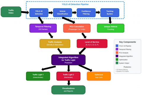
Figure 16. Classification framework of our proposed work
Figure 16 illustrates the classification framework of the proposed intelligent traffic management system. The workflow initiates with video input feeding into the YOLOv8 pipeline (blue dashed box), encompassing detection, classification, confidence filtering, and vehicle tracking. The framework branches into parallel streams: temporal filtering, PCU calculation for standardized units, and unique vehicle counting. The analysis module processes density and saturation, while the level of service component evaluates conditions using standard classifications (A-F). These inputs converge into the integrated algorithm generating optimized timing for dual signals and total cycle calculations. The system concludes with visualizations and traffic management reports.
This section presents comprehensive evaluation results of the proposed intelligent traffic light optimization system. The analysis encompasses YOLOv8 model training performance metrics, computational efficiency analysis, real-world detection validation under diverse environmental conditions, and traffic signal optimization algorithm effectiveness. Results demonstrate the system's robustness across varying traffic scenarios, weather conditions, and lighting environments typical of historic urban centers, validating both detection accuracy and practical implementation viability for adaptive traffic management.
4.1 Training results – 126 epochs
The detection performance metrics for all vehicle classes are summarized in Table 3, which presents the mAP50 and mAP50-95 results demonstrating the model's accuracy across different confidence thresholds.
Table 3. mAP50 and mAP50-95 results
|
Specific Classes |
mAP50 |
mAP50-95 |
|
Clase A Clase MB Clase M Clase CP Clase RC Clase PU Clase MT Clase CG |
0.954 0.964 0.921 0.815 0.772 0.891 0.975 0.842 |
0.836 0.852 0.719 0.71 0.687 0.809 0.928 0.792 |
Table 4. Precision and recall results
|
Specific Classes |
Precision |
Recall |
|
Clase A Clase MB Clase M Clase CP Clase RC Clase PU Clase MT Clase CG |
0.953 0.970 0.938 0.864 0.745 0.822 0.975 0.815 |
0.882 0.918 0.859 0.723 0.621 0.843 0.957 0.919 |
Additionally, Table 4 provides detailed precision and recall values for each specific vehicle class, demonstrating the model's classification accuracy and its ability to correctly identify different vehicle types under diverse traffic conditions.
Hardware Configuration:
- GPU: NVIDIA A100-SXM4-40GB (Google Colab)
- Input size: 640 × 640 pixels
- Batch size: 16
4.2 Model performance under varying conditions
The model was evaluated using 32 video recordings representing a wide range of traffic scenarios, with the goal of establishing optimized traffic light cycles based on vehicle demand.
Table 5. Processing times performance metrics
|
Stage |
Speed |
|
Preprocessing Inference Postprocessing |
0.1 ms (val) /0.3 ms (train) 2.6 ms (val) /4.7 ms (train) 0.9 ms (val) /1.0 ms (train) |
The temporal distribution presented in Table 5 demonstrates comprehensive system evaluation across critical traffic periods and diverse environmental conditions characteristic of Ayacucho's historic center. The 17-hour monitoring framework strategically captures peak traffic scenarios including morning rush hours (07:48 AM), midday congestion (12:29–12:44 PM), and evening traffic intensification (17:17–19:52 PM), alongside challenging weather conditions including heavy rain with wind and varying precipitation intensities. This extensive testing protocol ensures robust validation of the detection system's performance under real-world operational conditions typical of historic urban centers, where environmental variability significantly impacts traffic monitoring effectiveness. The inclusion of diverse lighting conditions from cloudy dawn (05:44 AM) through sunset transitions (16:21–17:51 PM) to complete nighttime scenarios (18:48–22:48 PM) validates the system's adaptability to the full spectrum of operational requirements. Furthermore, the evaluation encompasses shadow interference from colonial architecture during sunny periods, demonstrating the system's resilience against the unique challenges posed by heritage urban environments with their characteristic narrow streets and historic building configurations.
The detection results presented in Table 6 confirm the system's exceptional accuracy and reliability across all evaluated environmental scenarios, with successful vehicle identification consistently achieved despite varying traffic densities ranging from minimal flow (7 vehicles) to high-congestion scenarios (24 vehicles per sequence). The comprehensive classification performance demonstrates remarkable consistency in identifying primary vehicle classes (A, MB, M) while maintaining precise detection of less frequent vehicle types including commercial vehicles (CP, RC, CG) and specialized transportation (PU, MT). These results validate the effectiveness of the 126-epoch training protocol and the robustness of the YOLOv8 architecture adaptation for historic urban traffic scenarios. The system's ability to maintain detection accuracy under adverse conditions including heavy precipitation, nighttime glare, and shadow interference from colonial buildings establishes its readiness for practical deployment in dynamic traffic environments. This validation demonstrates the system's capability to provide reliable data for traffic signal optimization, ensuring accurate counting and classification for adaptive traffic management in heritage centers.
The comprehensive evaluation of the traffic signal optimization system is presented through detailed performance analysis across multiple scenarios. Table 6 shows the video recording conditions and temporal distribution used for system evaluation across 32 different scenarios, covering diverse environmental conditions including cloudy, sunny, night, and precipitation conditions spanning 17 hours of continuous monitoring.
Table 6. Video recording conditions and temporal distribution for system evaluation
|
Video |
Time |
Condition |
|
1 2 3 4 5 6 7 8 9 10 11 12 13 14 15 16 17 18 19 20 21 22 23 24 25 26 27 28 29 30 31 32 |
05:44 AM 06:21 AM 06:31 AM 07:48 AM 09:07 AM 10:53 AM 11:14 AM 11:21 AM 12:29 PM 12:44 PM 14:56 PM 15:57 PM 16:21 PM 17:17 PM 17:51 PM 18:32 PM 18:33 PM 18:48 PM 18:51 PM 18:56 PM 19:52 PM 19:55 PM 19:57 PM 20:18 PM 20:28 PM 20:31 PM 20:33 PM 20:34 PM 21:05 PM 21:09 PM 22:02 PM 22:48 PM |
Cloudy dawn Cloudy Cloudy Cloudy Sunny Mid-morning Mid-morning Sunny with shadows Noon Cloudy Sunny with shadows Sunny with shadows Sunset Sunset Sunset Dusk Dusk Night Night Night Night Heavy rain/ wind Heavy rain Light rain Light rain Light rain Light rain Light rain Light rain Light rain Night Light rain |
Table 7 presents the detailed vehicle detection, classification, and counting results under varying environmental conditions, demonstrating successful identification across all evaluated scenarios with vehicle counts ranging from 7 to 24 per video sequence.
Table 7. Vehicle detection, classification, and counting results under varying conditions
|
Video |
Detection/ Classification |
Total |
|
1 2 3 4 5 6 7 8 9 10 11 12 13 14 15 16 17 18 19 20 21 22 23 24 25 26 27 28 29 30 31 32 |
A:7, MB:1, M:1, PU:2, MT:1 A:5, MB:3, M:2, MT:1 A:5, MB:1, M:3 A:8, MB:4, M:4, CP:1, PU:1 A:4, MB:1, M:3, PU:1 A:8, MB:6, M:2 A:8, MB:7, M:6 A:7, MB:4, M:6, PU:1, CG:1 A:4, MB:6, M:4, CP:1, PU:3 A:10, MB:5, M:5, PU:1 A:7, MB:2, M:10 A:7, MB:4, M:2, CP:1, PU:3, CG:1 A:10, MB:5, CP:1, PU:1 A:3, MB:3, M:8, CP:1, CG:1 A:8, MB:7, M:7, PU:1 A:4, MB:1, M:7, PU:1 A:4, MB:1, M:7, PU:1 A:7, MB:5, M:6, RC:1, PU:1 A:3, MB:1, M:8 A:12, MB:3, M:3 A:6, MB:3, M:9, RC:1, PU:1, CG:3 A:7, MB:3, M:6, PU:3 A:10, MB:2, M:9, PU:1, MT:1 A:8, MB:1, M:9 A:9, MB:1, M:1, CP:1 A:6, M:6, PU:1 A:2, MB:1, M:4 A:9, M:6 A:7, MB:2, M:8, PU:3 A:5, MB:9, RC:1, PU:1 A:6, MB:8 A:10, M:2 |
12 11 9 18 9 16 21 19 18 21 19 18 17 16 23 13 20 12 18 24 23 19 23 18 12 13 7 15 20 16 14 12 |
4.3 Detection performance across environmental scenarios
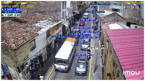
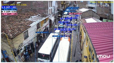
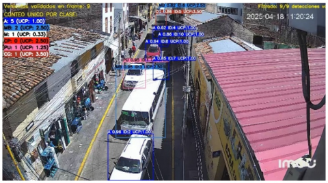
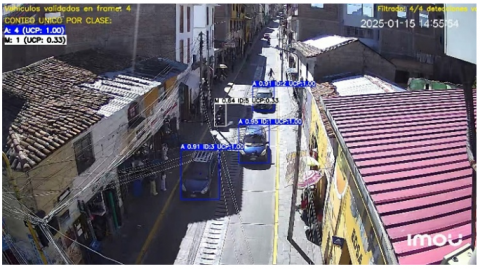
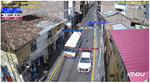
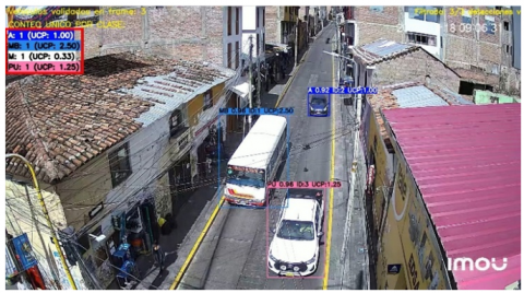
Figures 17-19 demonstrate the model's effectiveness under variable traffic conditions throughout different time periods and traffic densities. The results show correct detection with high confidence scores (ranging from 0.76 to 0.96), unique ID assignment for each vehicle type, UCP (PCU) values for comprehensive traffic analysis, and in the upper left corner, the counting records displaying real-time vehicle tallies by class with cumulative totals. Figure 17 illustrates optimal performance under light traffic conditions with clear vehicle separation and precise bounding box placement. Figure 18 shows the maintained accuracy during medium traffic density with successful detection of overlapping vehicles and accurate classification despite increased scene complexity. Figure 19 validates robust performance under high-density traffic scenarios where vehicles are closely positioned, demonstrating the system's capability to distinguish individual vehicles even in congested conditions. This comprehensive visualization validates the system's capability to maintain accurate detection and classification performance across light, medium, and high-density traffic scenarios typical of historic urban centers, confirming the model's adaptability to real-world operational requirements and establishing its reliability for practical traffic management applications.
Figure 17. Performance under light traffic scenarios
Figure 18. Performance under medium traffic conditions
Figure 19. Performance under high-density traffic
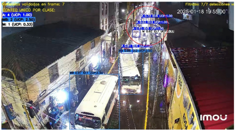
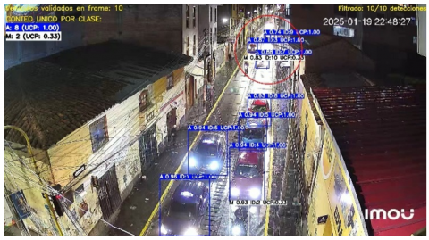
Figures 20-22 demonstrate the system's robust performance under challenging nighttime conditions with varying vehicle light glare and precipitation intensity, scenarios particularly relevant to Ayacucho where rainfall is frequent during December-March seasons. These sequential images, captured during evening hours (19:55–22:48), showcase the model's adaptability to progressively challenging rainy season conditions. The red circles highlight glare interference points from vehicle headlights, demonstrating the system's capability to maintain accurate detection despite these visual obstacles. Figure 20 illustrates effective detection under light rain with moderate glare, maintaining high confidence scores (0.62–0.98). Figure 21 shows sustained performance under medium precipitation and glare, with accurate identification of multiple vehicle classes (A, MB, M, PU) despite increased interference. Figure 22 validates exceptional resilience under intense conditions with heavy glare and adverse weather, demonstrating maintained detection accuracy when visibility is severely compromised. The consistent vehicle counting (7–10 detections per frame) and reliable classification confirm the system's operational reliability for deployment in Ayacucho's historic center, where narrow streets intensify lighting challenges and seasonal rainfall creates visibility complications.
Figure 20. Effectiveness against vehicle light glare and light rain conditions
Figure 21. Effectiveness against vehicle light glare and light medium conditions
Figure 22. Effectiveness against vehicle light glare and light intense conditions
Figure 23. Effectiveness against shadow conditions, showing temporal filtering of false positives
Figure 24. Effectiveness against shadow conditions
Figures 23 and 24 demonstrate the system's effectiveness against shadow conditions caused by Ayacucho's colonial mansions, showcasing temporal filtering for false positive elimination. Figure 23 illustrates dynamic classification refinement, where the small truck counter (CP) shows zero because the system correctly reclassified the vehicle as a large truck (CG) as it approached closer. This adaptive classification demonstrates temporal filtering's capability to improve detection accuracy by continuously evaluating vehicle characteristics across frames. The system successfully detects 9 vehicles with high confidence scores (0.62–0.98) despite shadow interference. Figure 24 validates sustained performance with 4 detected vehicles, maintaining reliable classification (A, M) with confidence scores above 0.84. Both images confirm the system's robustness against shadow interference typical of narrow historic streets, validating the model's adaptability to heritage urban center challenges.
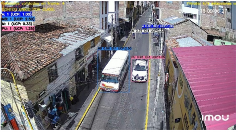
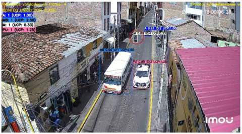
Figures 25-27 demonstrate the system's occlusion handling capability in confined urban spaces where smaller vehicles frequently become hidden behind larger ones. Through temporal tracking that assigns unique identification codes to each detected vehicle, the system maintains accurate records even when vehicles temporarily disappear from view. Figure 25 shows initial motorcycle detection at 09:06:28 am with clear visibility and high confidence (0.92). Figure 26 captures the critical moment at 09:06:30 am when the motorcycle is about to be occluded by the microbus. Figure 27 illustrates complete occlusion at 09:06:31 am where the motorcycle remains registered in the counting system despite being entirely hidden. This sequence confirms the system's capability to handle challenging detection scenarios in historic urban centers, where narrow streets and mixed vehicle sizes create frequent occlusion situations.
Figure 25. Initial motorcycle detection before occlusion
Figure 26. Motorcycle tracking during partial occlusion
Figure 27. Motorcycle detection loss due to complete occlusion
4.4 Results of the traffic signal optimization algorithm
The traffic signal optimization results are presented through comprehensive quantitative analysis across multiple metrics. Table 8 summarizes the vehicle count and accumulated PCU values for traffic analysis across 32 evaluation scenarios. Table 9 presents the PCU density and saturation degree metrics, which are fundamental for determining service levels and establishing optimization parameters for traffic signal control. Table 10 details the applied increments and PCU factor adjustments used in the optimization algorithm, demonstrating algorithm adaptation to varying traffic conditions with increments ranging from 4.3% to 25.0%. Table 11 displays the traffic flow service levels and PCU density classification for all evaluated scenarios, ranging from free flow (Level A) to unstable flow (Level E), validating the system's effectiveness in moderate to low congestion scenarios typical of historic urban centers. Finally, Table 12 presents the optimized traffic signal timing results, including green time, amber time, and red time for both traffic lights, with green light timing ranging from 20.3 to 40.5 seconds and amber phases of 3.6-4.2 seconds corresponding to the proportional traffic demands.
The service level evaluation represents an adaptation of standard traffic engineering criteria customized for the specific conditions of Ayacucho's historic center. The level of service (A-F) is calculated based on PCU density using adapted thresholds that reflect the unique operational constraints of heritage urban environments. This customized classification system modifies traditional Highway Capacity Manual standards to account for the narrow street configurations, mixed vehicle types, and operational limitations characteristic of colonial urban layouts. The algorithm evaluates traffic conditions using density-based criteria where Level A (free flow) corresponds to PCU densities below 9, Level B (stable reasonable flow) ranges from 9-14, and subsequent levels increase proportionally to accommodate the specific traffic patterns observed in historic city centers. This adaptation ensures accurate service level assessment under conditions not fully addressed by conventional traffic analysis methods, providing a more precise evaluation framework for heritage urban traffic management systems.
Table 8. Vehicle count and accumulated PCU values for traffic analysis
|
Video |
Total Vehicle |
Accum. PCU Value |
|
1 2 3 4 5 6 7 8 9 10 11 12 13 14 15 16 17 18 19 20 21 22 23 24 25 26 27 28 29 30 31 32 |
12 11 9 18 9 16 21 19 18 21 19 18 17 16 23 13 20 12 18 24 23 19 23 18 12 13 7 15 20 16 14 12 |
13.08 13.91 8.49 23.07 8.74 23.66 27.48 23.73 26.57 25.40 15.30 27.41 26.25 19.14 29.06 10.06 24.73 8.14 20.49 18.12 30.22 20.23 19.97 13.47 14.33 9.23 5.82 10.98 18.39 11.22 8.64 10.66 |
Table 9. PCU density and saturation degree metrics
|
Video |
´PCU Density |
Saturation Degree |
|
1 2 3 4 5 6 7 8 9 10 11 12 13 14 15 16 17 18 19 20 21 22 23 24 25 26 27 28 29 30 31 32 |
1.07 1.09 0.67 1.83 0.69 1.86 2.17 1.82 2.12 2.02 1.21 2.17 2.07 1.51 2.31 0.82 1.94 0.64 1.62 1.45 2.39 1.88 1.58 1.13 1.12 0.77 0.46 0.89 1.46 0.90 0.69 0.87 |
0.56 0.58 0.35 0.96 0.36 0.98 1.00 0.96 1.00 1.00 0.64 1.00 1.00 0.80 1.00 0.43 1.00 0.34 0.85 0.76 1.00 0.99 0.83 0.59 0.59 0.41 0.24 0.47 0.77 0.47 0.36 0.46 |
Table 10. Applied increments and PCU factor adjustments
|
Video |
Applied Increment |
PCU Factor |
|
1 2 3 4 5 6 7 8 9 10 11 12 13 14 15 16 17 18 19 20 21 22 23 24 25 26 27 28 29 30 31 32 |
11.3% 11.5% 6.4% 24.1% 6.5% 24.5% 25.0% 23.9% 25.0% 25.0% 12.8% 25.0% 25.0% 15.9% 25.0% 7.7% 25.0% 6.1% 21.3% 15.2% 25.0% 24.7% 20.8% 11.8% 11.8% 7.3% 4.3% 8.5% 15.4% 8.5% 6.5% 8.3% |
1.00% 1.00% 1.00% 1.00% 1.00% 1.00% 1.10% 1.00% 1.06% 1.02% 1.00% 1.10% 1.05% 1.00% 1.16% 1.00% 1.00% 1.00% 1.00% 1.00% 1.20% 1.00% 1.00% 1.00% 1.00% 1.00% 1.00% 1.00% 1.00% 1.00% 1.00% 1.00% |
Table 11. Traffic flow service levels and PCU density classification
|
Video |
Lebel of Service |
PCU Density |
|
1 2 3 4 5 6 7 8 9 10 11 12 13 14 15 16 17 18 19 20 21 22 23 24 25 26 27 28 29 30 31 32 |
B-Stable flow (reasonable) B-Stable flow (reasonable) A-Free flow D-Near-unstable flow A-Free flow D-Near-unstable flow E-Unstable flow D-Near-unstable flow E-Unstable flow E-Unstable flow C-Stable flow E-Unstable flow E-Unstable flow C-Stable flow E-Unstable flow B-Stable flow (reasonable) E-Unstable flow A-Free flow D-Near-unstable flow C-Stable flow C-Stable flow B-Stable flow (reasonable) D-Near-unstable flow C-Stable flow C-Stable flow B-Stable flow (reasonable) A-Free flow B-Stable flow (reasonable) C-Stable flow B-Stable flow (reasonable) A-Free flow B-Stable flow (reasonable) |
1.07 1.09 0.67 1.83 0.69 1.86 2.17 1.82 2.12 2.02 1.21 2.17 2.07 1.51 2.31 0.82 1.94 0.64 1.62 1.45 2.39 1.88 1.58 1.13 1.12 0.77 0.46 0.89 1.46 0.90 0.69 0.87 |
Table 12. Optimized traffic signal timing results
|
Video |
Green Time-Light 01 |
Amber Time-Light 01 |
Red Time-Light 02 |
|
1 2 3 4 5 6 7 8 9 10 11 12 13 14 15 16 17 18 19 20 21 22 23 24 25 26 27 28 29 30 31 32 |
26.4 26.6 22.0 36.8 22.2 37.1 39.0 36.7 38.4 37.7 27.5 38.9 38.2 30.3 39.9 24.2 37.5 21.8 34.8 29.7 40.5 37.3 32.0 26.8 26.8 22.8 20.3 24.8 29.8 24.8 22.1 24.6 |
3.9 3.9 3.7 4.2 3.7 4.2 4.2 4.2 4.2 4.2 4.0 4.2 4.2 4.1 4.2 3.8 4.2 3.7 4.1 4.0 4.2 4.2 4.1 3.9 3.9 3.8 3.6 3.8 4.1 3.8 3.7 3.8 |
31.3 31.5 26.7 42 26.9 42.3 44.2 41.8 43.6 42.9 32.4 44.1 43.5 35.4 45.1 29.0 42.7 26.5 39.9 34.8 45.7 42.5 37.1 31.7 31.7 27.5 24.9 29.6 34.9 29.6 26.8 29.5 |
4.5 Validation methodology analysis
The dataset was divided using a 70/30 random split to ensure representative distribution of both camera perspectives (frontal and inclined), diverse temporal conditions, and vehicular classes across both training and validation sets. This methodology is particularly appropriate given that data originates from two distinct camera configurations with complementary perspectives, ensuring that the model learns visual robustness against different vehicular capture angles typical of historic center intersections.
The random partitioning approach enables the model to generalize across the full spectrum of environmental and geometric conditions captured during the study period, including variations in lighting, weather conditions (sunny, cloudy, rainy scenarios), time periods (dawn, midday, sunset, nighttime), and the unique challenges posed by colonial architecture shadows. This comprehensive exposure during both training and validation phases enhances the model's adaptability to the complex visual scenarios’ characteristic of heritage urban environments, where fixed camera positions must accommodate diverse traffic patterns and environmental variability.
In this work, we propose an intelligent traffic light system to address vehicular congestion in the historic center of Ayacucho. Our proposed system efficiently detects, classifies, and counts vehicles even under heterogeneous conditions, including variable traffic patterns, diverse environmental factors (precipitation, fluctuating sunlight, projected shadows), and low-visibility nighttime scenarios. The implementation of an advanced temporal filtering system has proven essential for distinguishing real objects from environmental artifacts, thereby preserving the integrity of vehicle tracking through the assignment of unique, persistent identifiers across frames. Additionally, the trajectory visualization feature, using color-coded paths differentiated by vehicle type, enhances visual validation and supports intuitive monitoring of traffic flow.
The implementation of this system has the potential to resolve multiple urban issues by optimizing critical resources such as time and energy, while also producing substantial economic savings that can benefit a country's economy. The 13-stage traffic signal optimization algorithm demonstrates effectiveness in adapting to real-time vehicular demand, achieving significant improvements in traffic flow efficiency compared to traditional fixed-time systems.
However, the current algorithm focuses primarily on vehicular traffic optimization. Future research should incorporate pedestrian traffic considerations, including minimum walk times, pedestrian clearance intervals, and multi-modal demand detection, to develop a comprehensive traffic management system that addresses both vehicular and pedestrian flows in heritage urban environments. Additionally, integration with emergency vehicle prioritization and coordination with adjacent intersections represents important areas for system enhancement.
This research was conducted at a single intersection due to resource constraints inherent to self-funded academic research. The acquisition of additional high-quality cameras for multiple intersection validation was economically unfeasible, while existing municipal surveillance infrastructure proved inadequate for computer vision analysis due to poor image quality and suboptimal positioning angles. The selected intersection represents a critical bottleneck in Ayacucho's historic center traffic network, chosen because traffic flow optimization at this point directly impacts upstream and downstream circulation patterns throughout the heritage zone. Future research will extend validation to diverse intersection configurations including three-way confluences, four-way intersections, and roundabout-integrated traffic signals, while the current single-intersection validation provides proof-of-concept for the adaptive algorithm.
As a future projection, we aim to design an intelligent traffic signal controller that acts as an interface between the analytical model and the physical traffic light infrastructure, enabling the real-time and dynamic application of the signal cycles computed by the system.
[1] Abbas, S.K., Khan, M.U.G., Zhu, J., Sarwar, R., Aljohani, N.R., Hameed, I.A., Hassan, M.U. (2024). Vision based intelligent traffic light management system using Faster R-CNN. CAAI Transactions on Intelligence Technology, 9(4): 932-947. https://doi.org/10.1049/cit2.12309
[2] Imisiker, S., Tas, B.K.O., Yildirim, M.A. (2019). Stuck on the road: Traffic congestion and stock returns. SSRN Electronic Journal. https://ssrn.com/abstract=2933561.
[3] Chowdhury, M., Hasan, M., Safait, S. (2018). A novel approach to forecast traffic congestion using CMTF and machine learning. B.Sc. Thesis, BRAC University, Dhaka, Bangladesh.
[4] Transitemos Foundation. (2017). Aspectos Negativos de la Congestión Vehicular: Impacto social y económico. Transitemos Foundation, Lima, Peru.
[5] Fonseca, N., Casanova, J., Valdés, M. (2011). Influence of the stop/start system on CO emissions of a diesel vehicle in urban traffic. Transportation Research Part D: Transport and Environment, 16(2): 194-200. https://doi.org/10.1016/j.trd.2010.10.001
[6] Sutandi, A.C. (2009). ITS impact on traffic congestion and environmental quality in large cities in developing countries. In Proceedings of the Eastern Asia Society for Transportation Studies, p. 180. https://doi.org/10.11175/eastpro.2009.0.180.0
[7] Prayitno, A., Indrawati, V., Yusuf, Y.G. (2024). Synchronization of heterogeneous vehicle platoon using distributed PI controller designed based on cooperative observer. Mathematical Modelling of Engineering Problems, 11(6): 1558-1566. https://doi.org/10.18280/mmep.110616
[8] Wang, C., Shang, Q., Liu, K., Zhang, W. (2025). Traffic congestion recognition based on convolutional neural networks in different scenarios. Engineering Applications of Artificial Intelligence, 148: 110372. https://doi.org/10.1016/j.engappai.2025.110372
[9] Kiran, K.V., Dash, S., Parida, P. (2024). Vehicle detection in varied weather conditions using enhanced deep YOLO with complex wavelet. Engineering Research Express, 6(2): 025224. https://doi.org/10.1088/2631-8695/ad507d
[10] Xu, S., Zhang, M., Zhong, Y. (2024). YOLO-HyperVision: A vision transformer backbone-based enhancement of YOLOv5 for detection of dynamic traffic information. Egyptian Informatics Journal, 27: 100523. https://doi.org/10.1016/j.eij.2024.100523
[11] Lin, C.J., Lee, C.M. (2024). Real-time vehicles detection with YOLOv8. In Proceedings of the 11th IEEE International Conference on Consumer Electronics – Taiwan, Taiwan, pp. 805-806. https://doi.org/10.1109/ICCE-Taiwan62264.2024.10674607
[12] Macherla, H., Muvva, V.R., Lella, K.K., Palisetti, J.R., Pulugu, D., Vatambeti, R. (2024). A deep reinforcement learning-based RNN model in a traffic control system for 5G-envisioned internet of vehicles. Mathematical Modelling of Engineering Problems, 11(1): 75-83. https://doi.org/10.18280/mmep.110107
[13] Duc, Q.N., Kim, T.D., Nguyen, Q., Thi, T.H.N., Vu, Q., Xuan, M.D. (2024). Optimizing traffic light control using YOLOv8 for real-time vehicle detection and traffic density. In 2024 9th International Conference on Integrated Circuits, Design, and Verification (ICDV), Hanoi, Vietnam, pp. 119-124. https://doi.org/10.1109/ICDV61346.2024.10616901
[14] Naithani, A., Jain, V. (2024). Real-time crossroad traffic light management. In 2024 8th International Symposium on Innovative Approaches in Smart Technologies (ISAS), İstanbul, Turkiye, pp. 1-6. https://doi.org/10.1109/ISAS64331.2024.10845613
[15] Saseendran, A., Worin, J., Jyothika, K.J., Ravindran, R.C. (2025). Automated traffic signal system incorporating real-time traffic. In Cognizant Transportation Systems: Challenges and Opportunities. IMPACTS 2023. Lecture Notes in Civil Engineering, vol. 263. Springer, Singapore. https://doi.org/10.1007/978-981-97-7300-8_40
[16] Rashad, M.F., Ali, Q.I. (2025). Deploying Android-based smart RSUs with YOLOv8 and SAHI for enhanced traffic management. Diyala Journal of Engineering Sciences, 18(1): 70-90. https://doi.org/10.24237/djes.2025.18104
[17] Pudaruth, S., Boodhun, I.M., Onn, C.W. (2024). Reducing traffic congestion using real-time traffic monitoring with YOLOv8. International Journal of Advanced Computer Science and Applications, 15(10): 1068-1079. https://doi.org/10.14569/IJACSA.2024.01510109
[18] Li, H., Lv, J. (2024). Research on traffic vehicle target tracking method based on YOLO algorithm and ResNet. In Proceedings of the 2024 9th International Conference on Cyber Security and Information Engineering (ICCSIE), Kuala Lumpur, Malaysia, pp. 757-761. https://doi.org/10.1145/3689236.3695379
[19] Bui, T., Wang, G., Wei, G., Zeng, Q. (2024). Vehicle multi-object detection and tracking algorithm based on improved You Only Look Once 5s version and DeepSORT. Applied Sciences, 14(7): 2690. https://doi.org/10.3390/app14072690
[20] Azimjonov, J., Özmen, A., Kim, T. (2023). A nighttime highway traffic flow monitoring system using vision-based vehicle detection and tracking. Soft Computing, 27: 13843-13859. https://doi.org/10.1007/s00500-023-08860-z
[21] Rasheed, R., Puma, J.C.T., Kulothungan, K., Kathirvelu, B., Subramanian, S., Tripathi, V. (2024). Identification and counting of vehicles in real time for expressway. AIP Conference Proceedings, 2937(1): 020035. https://doi.org/10.1063/5.0218184
[22] Patil, A., Raorane, A., Kundale, J. (2023). Enhancing traffic management with deep learning-based vehicle detection and scheduling systems. In 2023 International Conference on Modeling, Simulation & Intelligent Computing (MoSICom), Dubai, United Arab Emirates, pp. 223-227. https://doi.org/10.1109/MoSICom59118.2023.10458787
[23] Kunekar, P., Narule, Y., Mahajan, R., Mandlapure, S., Mehendale, E., Meshram, Y. (2023). Traffic management system using YOLO algorithm. Engineering Proceedings, 59(1): 210. https://doi.org/10.3390/engproc2023059210
[24] Pujari, S., Kumar, A. (2024). AI-enabled road traffic flow control and mobility prediction using YOLO. In Artificial Intelligence for Wireless Communication Systems. CRC Press.
[25] Lavanya, K., Tiwari, S., Anand, R., Hemanth, J. (2023). YOLO and LSH-based video stream analytics landscape for short-term traffic density surveillance at road networks. Turkish Journal of Electrical Engineering and Computer Sciences, 31(6): 1099-1112. https://doi.org/10.55730/1300-0632.4036
[26] Ottom, M.A., Al-Omari, A. (2023). An adaptive traffic lights system using machine learning. The International Arab Journal of Information Technology, 20(3): 407-415. https://doi.org/10.34028/iajit/20/3/13
[27] Salekin, S.U., Ullah, M.H., Khan, A.A.A., Jalal, M.S., Nguyen, H.H., Farid, D.M. (2024). Bangladeshi native vehicle classification employing YOLOv8. In Intelligent Systems and Data Science. ISDS 2023. Communications in Computer and Information Science, vol. 1949. Springer, Singapore. https://doi.org/10.1007/978-981-99-7649-2_14
[28] Hendrawan, A., Gernowo, R., Nurhayati, O.D., Dewi, C. (2024). A novel YOLO-ARIA approach for real-time vehicle detection and classification in urban traffic. International Journal of Intelligent Engineering and Systems, 17(1): 428-438. https://doi.org/10.22266/ijies2024.0229.38
[29] Arafat, M.Y., Adnan, M.F., Islam, M.F. (2023). AI-based affordable high-density traffic monitoring system. In 2023 International Conference on Next-Generation Computing, IoT and Machine Learning (NCIM), Gazipur, Bangladesh, pp. 1-5. https://doi.org/10.1109/NCIM59001.2023.10212910
[30] Anwar, S.A., Zohura, F.T., Paul, J. (2023). Intelligent traffic control system using computer vision algorithms. In Proceedings of SPIE: Optics and Photonics for Information Processing XVII, 12673: 1267306, San Diego, California, USA. https://doi.org/10.1117/12.2682676
[31] Jain, S., Indu, S., Goel, N. (2023). Comparative analysis of YOLO algorithms for intelligent traffic monitoring. In Proceedings on International Conference on Data Analytics and Computing. ICDAC 2022. Lecture Notes on Data Engineering and Communications Technologies, vol. 175. Springer, Singapore. https://doi.org/10.1007/978-981-99-3432-4_13
[32] Transportation Research Board. (2016). Highway Capacity Manual 6th Edition: A Guide for Multimodal Mobility Analysis. Washington, DC: The National Academies Press. https://doi.org/10.17226/24798
[33] Webster, F.V. (1958). Traffic Signal Settings. Road Research Technical Paper No. 39. Road Research Laboratory, Her Majesty's Stationery Office, London.
[34] Kell, J.H., Fullerton, I.J. (1991). Manual of Traffic Signal Design. Institute of Transportation Engineers, Washington, DC, USA.
[35] Institute of Transportation Engineers (ITE). (1991). Manual of Traffic Signal Design. Second Edition. Washington, DC, United States.
[36] Brosseau, M., Zangenehpour, S., Saunier, N., Miranda-Moreno, L. (2013). The impact of waiting time and other factors on dangerous pedestrian crossings and violations at signalized intersections: A case study in Montreal. Transportation Research Part F: Traffic Psychology and Behaviour, 21: 159-172. https://doi.org/10.1016/j.trf.2013.09.010
[37] Akçelik, R. (1980). Time-Dependent Expressions for Delay, Stop Rate and Queue Length at Traffic Signals. Internal Report AIR 367-1. Australian Road Research Board, Vermont South, Australia.