H. A. Bhavithra![]() | D. Kavitha
| D. Kavitha![]() | J. Shobana
| J. Shobana![]() | M. Nila
| M. Nila![]() | S. Sindu Devi*
| S. Sindu Devi*![]()
© 2025 The authors. This article is published by IIETA and is licensed under the CC BY 4.0 license (http://creativecommons.org/licenses/by/4.0/).
OPEN ACCESS
This study develops a mathematical model to understand the spread of measles using the classical Susceptible–Infected–Recovered (SIR) framework, incorporating vaccination as a key control strategy. The model is analyzed to identify equilibrium points and assess the stability of both the disease-free and endemic states. The analysis shows that the system undergoes a forward bifurcation at the critical threshold where the infection begins to persist in the population. We calculate the minimum vaccination coverage required to eliminate the disease. It was found that, when the basic reproduction number is 4.5, at least 77.78 percent of the population must be vaccinated to prevent sustained transmission. Numerical simulations are carried out using the Variational Iteration Method and Runge-Kutta, which provide accurate approximations of the disease dynamics. The results demonstrate that increasing vaccination coverage significantly lowers the number of infections and delays outbreak peaks. Overall, this study highlights the importance of high vaccination rates in controlling measles and shows the effectiveness of advanced numerical techniques in modeling infectious diseases.
SIR model, stability analysis, reproduction number, bifurcation parameter, critical vaccination proportion, transcritical bifurcation
Measles is a highly contagious viral disease that poses a significant public health challenge, particularly in regions with low vaccination coverage. Despite the availability of an effective vaccine, measles continues to cause outbreaks worldwide, especially in areas where immunization efforts are insufficient or inconsistent. Understanding the transmission dynamics of measles is crucial for designing effective control strategies and informing public health policies.
Agusto [1] explored the mathematical model for ebola virus and its stimulations. Althaus et al. [2] estimated the basic reproduction number for the Ebola virus through transmission rate. Chowell et al. [3] offered a comprehensive overview of mathematical models applied to Ebola’s transmission and containment. D’Silva and Eisenberg [4] used spatial invasion framework, incorporating local and cross regional transmission using gravity-based model approach. Li [5] developed a model for Ebola virus in Sierra Leone, emphasizing the influence of human movement on viral dissemination. Njankou and Nyabadza [6] constructed an optimal model control to access the awareness campaigns and medical interventions. Rachab and Torres [7] adopted simulation driven optimal control models to evaluate vaccine deployment strategies during the 2014 epidemic.
Dia et al. [8] introduced a modified Susceptible- Exposed-Infected-Recovered frame work to detailed the epidemic behaviour in Liberia. Meanwhile Sedelnikov [9] explored the fuzzy logic in disciplines like space science and engineering. Coltart et al. [10] traced the trajectory of 2013-2016 west African Ebola, outbreak highlighting the importance of data centric decision making and control measures. Barros et al. [11] studied the use of fuzzy dynamic system in epidemic modelling, while Farahi and Barati [12] applied fuzzy methodologies in time delayed system in epidemiology. Das and Pal [13] focused on Susceptible–Infected–Recovered (SIR) models with treatment strategies under fuzzy condition. Verma et al. [14] introduced fuzzy based model to analyze influence transmission and control. Sadhukhan et al. [15] explored optimal harvesting in a trophic model within a fuzzy logic framework. Bhavithra et al. [16, 17] examined parameters like basic reproduction number, backward, forward, transcritical bifurcation analysis as well as sensitivity analysis for SEIR model using sinusoidal function.
Sedelnikov et al. [18] also addressed interpretation challenges in telemetry data from the Advanced Industrial Science and Technology small satellite. Ahmad et al. [19] designed a fractional order COVID 19 model using Caputo derivatives. Yadav et al. [20] reviewed common epidemic model such as SI, SIR, SEIR analyzing key parameters particularly basic reproduction number forecasting in COVID 19 trends. Gurjar et al. [21] investigated the SIR model for COVID 19 in Indonesia, emphasising how face to face learning and vaccination affected transmission. Dwivedi et al. [22] constructed a nonlinear deterministic model to analyse the co-circulation of Japanese encephalitis and dengue. Bifurcation analysis for novel fuzzy SIR model has been studied by Bhavithra et al. [23].
Mathematical modeling plays a vital role in the study of infectious diseases by helping to predict disease spread, assess intervention strategies, and estimate key epidemiological thresholds. Among various modeling approaches, the SIR model is widely used for analyzing diseases like measles due to its simplicity and effectiveness in capturing core transmission dynamics. The basic reproduction number, often denoted as R-naught, serves as a critical threshold parameter that determines whether an infectious disease can invade and persist in a population. If the value is greater than one, the disease can spread; if it is less than one, the infection will eventually die out.
Several studies have extended the basic SIR model by including factors such as vaccination, birth and death rates, time delays, and age structure. Vaccination, in particular, has been incorporated into many models to determine the critical vaccination coverage needed to achieve herd immunity and eradicate the disease. Previous works have also employed various numerical methods to solve these models, including Runge-Kutta methods, finite difference schemes, and spectral collocation techniques. However, there is a growing need for efficient and accurate numerical approaches that can handle the nonlinear nature of these models. In this study, we develop a measles transmission model based on the SIR framework with the inclusion of a vaccination term. We analyze the system to determine the equilibrium points and their stability, and we perform a bifurcation analysis to understand the transition between disease-free and endemic states. We also apply the Variational Iteration Method and Runge Kutta method to obtain accurate numerical approximations of the system's behavior. The results provide insights into the role of vaccination in controlling measles and demonstrate the effectiveness of the proposed numerical approach.
The equation for $\frac{d s}{d t}$ describes the change in the susceptible population over time. The term $(1-p) N \pi$ represents the number of new susceptible individuals entering the population through natural births (fertility) while accounting for the vaccination rate $P$. The term $-\beta S I$ captures the loss of susceptible individuals due to interactions with the infected population $\boldsymbol{I}$, indicating the transmission of the disease. Finally, the term $-\pi S$ accounts for the natural mortality of susceptible individuals. Together, these components illustrate how the susceptible population evolves, factoring in births, infections, and mortality.
$\frac{d S}{d t}=(1-p) N \pi-\beta S I-\pi S$
The equation for $\frac{d I}{d t}$ represents the dynamics of the infected population over time. The term $\beta S I$ indicates the rate of new infections, where $\beta$ is the transmission rate and $S$ is the number of susceptible individuals, while $\boldsymbol{I}$ is the number of infected individuals. This captures how interactions between susceptible and infected individuals lead to new infections. The term $-(\gamma+\pi) I$ accounts for the loss of infected individuals, where $\gamma$ represents the recovery rate (those who return to a susceptible state) and $\pi$ reflects the natural mortality rate among the infected. Together, these components illustrate how the infected population grows through new infections and decreases due to recovery and mortality.
$\frac{d I}{d t}=\beta S I-(\gamma+\pi) I$
The equation for $\frac{d R}{d t}$ describes the change in the recovered population $R$ over time. The term $p N \pi$ represents the influx of recoveries from vaccinations, where $p$ is a parameter affecting the effectiveness of vaccines and $N$ is the total population, with $\pi$ being the fertility rate that contributes newborns. The term $\gamma I$ accounts for individuals recovering from the infected population $\boldsymbol{I}$, reflecting the recovery dynamics of the disease. Conversely, the term $-\pi R$ denotes the natural decline of the recovered population due to mortality, suggesting that recovered individuals can also die at a certain rate. Together, these components illustrate how the recovered population is influenced by births, recoveries, and mortality, creating a dynamic interplay that shapes public health outcomes. Overview of the parameters are given in Table 1.
$\frac{d R}{d t}=p N \pi+\gamma I-\pi R$
Table 1. The overview of parameters
|
Parameter |
Description |
Values |
|
S |
Those who are susceptible |
1 |
|
I |
Those who are infected |
0 |
|
R |
Recovered people |
0 |
|
μ |
Rate of mortality from natural causes |
0.5 |
|
β |
Typical rate of interaction |
0.9 |
|
γ |
Rate of recovery |
2.04 |
|
π |
Fertility rate |
0.2 |
|
P |
yearly vaccinations for newborns |
0.9 |
2.1 Assumptions made in SIR model
2.2 Extensive analysis
We will examine the framework in two categories:
(i) Measles free equilibrium point
(ii) Endemic equilibrium point
(i) Measles free equilibrium point:
In the field of mathematical epidemiology, especially within SIR-based models, a measles-free equilibrium (MFE) represents a condition where no individuals in the population are infected. This implies that the disease is not present and cannot be transmitted further.
As there is no infection in the population, we have found MFE as $\mathrm{M}_0=((1-\mathrm{p}) \mathrm{N}, 0,0)$.
(ii) Endemic equilibrium point:
Endemic equilibrium points describe a stable state in epidemiological models where the disease remains present in the population over time at a constant level. Unlike the disease-free equilibrium, where infection is completely absent, the endemic equilibrium reflects a persistent presence of infection, with the rate of new infections balancing the rate of recoveries. This results in a steady number of infected individuals, indicating that the disease neither dies out nor causes large-scale outbreaks.
The endemic equilibrium is obtained by solving the following equations:
$\begin{gathered}(1-p) \pi-\beta S I-\pi S=0 \\ \beta S I-(\gamma+\pi) I=0 \\ p \pi+\gamma I-\pi R=0\end{gathered}$
The endemic equilibrium point is given by $M_1= \left(S_1, I_1, R_1\right)=\left(\frac{1-p}{R_n}, \frac{\pi}{\beta}\left(R_0-1\right), p+\frac{R_0-1}{\beta}\right)$.
2.3 Reproduction number and basic reproduction number
Basic Reproduction Number $\left(R_0\right)$: This is the average number of secondary infections produced by one infected individual in a completely susceptible population. It's a theoretical measure assuming that no one in the population is immune either through vaccination or previous infection, and that no public health measures (like social distancing) have been taken. A disease with an $R_0$ above 1 is expected to spread in a population, while an $R_0$ below 1 suggests the disease will eventually die out.
The reproduction number $R$ and basic reproduction number $R_0$ for our model is calculated using next generation matrix $R_0=F V^{-1}$ and we found that $F=\beta S, V^{-1}=\frac{1}{\gamma+\pi}, R_0=\frac{\beta}{\gamma+\pi}$.
2.4 Stability analysis
Stability analysis in mathematical modeling, including epidemiological models like the SIR model, is used to determine the behaviour of the system over time and whether its equilibrium points are stable or unstable. Stability analysis helps understand the long-term dynamics of the system and predict its response to perturbations or changes in parameters. We will examine both local and global stability analysis here.
(i) Local stability analysis:
In the context of mathematical models, particularly in the fields of dynamical systems and differential equations, local stability refers to the behaviour of a system in the vicinity of an equilibrium point. An equilibrium point is a state where the system doesn't change, meaning that once the system reaches this point, it remains there if undisturbed. The concept of local stability helps us understand how the system reacts to small disturbances or changes near this equilibrium.
The Jacobian of our model at measles free equilibrium point is given by
$\mathrm{J}=\left[\begin{array}{ccc}-\pi & -\beta(1-\mathrm{p}) & 0 \\ 0 & \beta(1-\mathrm{p})-\gamma-\pi & 0 \\ 0 & \gamma & -\gamma-\pi\end{array}\right]$
The characteristic equation is $|J-\lambda I|=0$.
$\left[\begin{array}{ccc}-\pi-\lambda & -\beta(1-\mathrm{p}) & 0 \\ 0 & \beta(1-\mathrm{p})-\gamma-\pi-\lambda & 0 \\ 0 & \gamma & -\gamma-\pi-\lambda\end{array}\right]=0$
The eigen value of the above characteristic equation is found to be $-\pi, \beta(1-p)-\gamma-\pi$ and $-\gamma-\pi$.
The sign of $\beta(1-p)-\gamma-\pi$ determines the local stability of disease-free equilibrium point. If $\beta(1-p)<-\gamma-\pi$, then all the eigen values are negative and the disease-free equilibrium point is locally asymptotically stable. If $\beta(1- \mathrm{p})>-\gamma-\pi$, then this eigen value is positive and the diseasefree equilibrium point is unstable.
(ii) Global stability analysis:
Global stability in mathematical models, particularly in the context of dynamical systems and differential equations, extends the concept of stability from local surroundings of an equilibrium point to the entire state space of the system. It deals with the behavior of solutions in response to perturbations not just near an equilibrium point, but from any initial condition within the system's domain.
An equilibrium point of a dynamical system is said to be globally stable if, no matter where in the state space the system starts from, it will eventually converge to this equilibrium point as time progresses to infinity.
Let us consider the Lyapunov function $\boldsymbol{V}_{\mathbf{1}}$ as $\boldsymbol{V}_{\mathbf{1}}(\mathrm{t}, \mathrm{S}, \mathrm{I}, \mathrm{R})= C_1 I$
$\begin{gathered}\frac{d V_1}{d t}=c_1 I^{\prime}, \frac{d V_1}{d t}=c_1[\beta S I-(\gamma+\pi) I] \\ \frac{d V_1}{d t}=c_1[\beta S-(\gamma+\pi)] I, \frac{d V_1}{d t} \leq c_1[\beta(1-\mathrm{p})-(\gamma+\pi)] I\end{gathered}$
Let $c_1=\frac{1}{\beta(1-p)-(\gamma+\pi)}$, thus $\frac{d V_1}{d t}=0$ iff $\mathrm{I}=0$. Now put $\mathrm{I}=0$ in model system of equation, we get $\mathrm{S} \rightarrow 1-\mathrm{p}$ and $\mathrm{R} \rightarrow 0$ as T $\rightarrow \infty$. By Lasalle's in-variance principle, $\boldsymbol{V}_{\mathbf{1}}$ is globally asymptotically stable.
The critical vaccination threshold, or the critical vaccination proportion, is a concept in epidemiology that indicates the fraction of a population that needs to be vaccinated to prevent an infectious disease from spreading within that population. This threshold is crucial for achieving herd immunity, where indirect protection from infectious disease is provided to unvaccinated individuals when a significant portion of the population is vaccinated.
The formula to find the critical vaccination proportion $\left(P_c\right)$ is derived from the reproduction number $\left(R_0\right)$, which is the average number of cases one infected individual will generate over the course of their infectious period in a completely susceptible population. The formula is: $P_c=1-\frac{1}{R_0}=1- \frac{\gamma+\pi}{\beta}$. If $P_c>p$, measles free equilibrium is locally stable with the coordinates $\mathrm{M}_0=(1-\mathrm{p}, 0,0)$.
Theorem 1:
Let S denote the susceptible population, I the infected population, and R the recovered population. Suppose the susceptible population S is four times the infection rate I, and the recovered population R is equal to the infection rate I. Let $\pi$ represent the fertility rate, γ denote the recovery rate and p denote the vaccination coverage for newborns. The following relationships hold for the rate of recovery γ as a function of the fertility rate π and the vaccination coverage p:
Here, $\propto$ denotes proportionality. These relationships describe how the rate of recovery $\boldsymbol{\gamma}$ varies with changes in the vaccination coverage $\mathbf{p}$ relative to the fertility rate $\boldsymbol{\pi}$.
Proof:
From our model we have,
$\frac{d S}{d t}=(1-\mathrm{p}) N(t) \pi-\beta \mathrm{SI}-\pi \mathrm{S}$ (1)
$\frac{d I}{d t}=\beta \mathrm{SI}-(\gamma+\pi) I$ (2)
$\frac{d R}{d t}=N(t) p \pi+\gamma I-\pi R$ (3)
Dividing Eq. (1) by Eq. (2), we get
$\frac{d S(t)}{d I(t)}=\frac{(1-\mathrm{p}) \mathrm{N}(\mathrm{t}) \pi-\beta \mathrm{SI}-\pi \mathrm{S}}{\beta \mathrm{SI}-(\gamma+\pi) I}$
$\frac{4 d I(t)}{d I(t)}=\frac{(1-\mathrm{p}) \pi 6 I(t)-4 \beta I(t) I(t)-4 \pi I(t)}{4 \beta I(t) I(t)-(\gamma+\pi) I(t)}$
$4=\frac{(1-p) \pi 6-4 \beta I(t)-4 \pi}{4 \beta I(t)-(\gamma+\pi)}$
$\begin{gathered}4[4 \beta I(t)-(\gamma+\pi)]=(1-\mathrm{p}) \pi 6-4 \beta I(t)-4 \pi \\ 16 \beta I(t)-4(\gamma+\pi)=(1-\mathrm{p}) \pi 6-4 \beta I(t)-4 \pi \\ 20 \beta I(t)=6(1-\mathrm{p}) \pi-4 \pi+4(\gamma+\pi)\end{gathered}$
$I(t)=\frac{6(1-p) \pi-4 \pi+4(\gamma+\pi)}{20 \beta}$ (4)
Dividing Eq. (1) by Eq. (3), we get
$\begin{gathered}\frac{d S(t)}{d R(t)}=\frac{(1-\mathrm{p}) \mathrm{N}(\mathrm{t}) \pi-\beta \mathrm{SI}-\pi \mathrm{S}}{N(t) p \pi+\gamma I-\pi R} \\ \frac{4 d I(t)}{d I(t)}=\frac{(1-\mathrm{p}) \pi 6 I(t)-4 \beta I(t) I(t)-4 \pi I(t)}{6 I(t) p \pi+\gamma I(t)-\pi I(t)} \\ 4=\frac{(1-\mathrm{p}) \pi 6-4 \beta I(t)-4 \pi}{6 p \pi+\gamma-\pi} \\ 4[6 p \pi+\gamma-\pi]=(1-\mathrm{p}) 6 \pi-4 \beta \mathrm{I}(\mathrm{t})-4 \pi \\ 4 \beta \mathrm{I}(\mathrm{t})=(1-\mathrm{p}) 6 \pi-4 \pi-4[6 p \pi+\gamma-\pi] \\ I(t)=\frac{6 \pi-4 \gamma-30 p \pi}{4 \beta}\end{gathered}$ (5)
Now Eqs. (4) and (5) we get,
$\frac{6(1-\mathrm{p}) \pi-4 \pi+4(\gamma+\pi)}{20 \beta}=\frac{6 \pi-4 \gamma-30 p \pi}{4 \beta}$
$6(1-p) \pi-4 \pi+4(\gamma+\pi)=5[6 \pi-4 \gamma-30 p \pi]$
$24 \gamma=24 \pi-144 p \pi, 24 \gamma=(24-144 p) \pi$
Now when $p=1$ (newborn vaccination is 100%): $\gamma= \frac{(24-144) \pi}{24} \propto-5 \pi$.
When $p=0.5$ (newborn vaccination is 50%): then $\gamma= \frac{(24-72) \pi}{24} \propto-2 \pi$.
When $p=1 / 3$ (newborn vaccination is approximately 33.33%): then $\gamma=\frac{(24-48) \pi}{24} \propto-\pi$.
Hence proved.
Theorem 2:
Let S denote the susceptible population, I the infected population, and R the recovered population. Suppose the susceptible population S is twice the infection rate I, and the recovered population R is equal to the infection rate I. Let π represent the fertility rate, γ denote the recovery rate and p denotes the vaccination coverage for newborns. The following relationships hold for the rate of recovery γ as a function of the fertility rate π and the vaccination coverage p:
Here, $\propto$ denotes proportionality. These relationships describe how the rate of recovery $\gamma$ varies with changes in the vaccination coverage $p$ relative to the fertility rate $\pi$.
Proof:
From our model we have,
$\frac{d S}{d t}=(1-\mathrm{p}) N(t) \pi-\beta \mathrm{SI}-\pi \mathrm{S}$ (6)
$\frac{d I}{d t}=\beta S I-(\gamma+\pi) I$ (7)
$\frac{d R}{d t}=N(t) p \pi+\gamma I-\pi R$ (8)
Dividing Eq. (6) by Eq. (7), we get
$\begin{gathered}\frac{d S(t)}{d I(t)}=\frac{(1-\mathrm{p}) \mathrm{N}(\mathrm{t}) \pi-\beta \mathrm{SI}-\pi \mathrm{S}}{\beta \mathrm{SI}-(\gamma+\pi) I} \\ \frac{2 d I(t)}{d I(t)}=\frac{(1-\mathrm{p}) \pi 4 I(t)-2 \beta I(t) I(t)-2 \pi I(t)}{2 \beta I(t) I(t)-(\gamma+\pi) I} \\ 2=\frac{4(1-\mathrm{p}) \pi-2 \beta I(t)-2 \pi}{2 \beta I(t)-(\gamma+\pi)} \\ 2[2 \beta I(t)-(\gamma+\pi)]=4(1-\mathrm{p}) \pi-2 \beta I(t)-2 \pi \\ 6 \beta I(t)=4 \pi-4 \pi p+2 \gamma \\ I(t)=\frac{4 \pi-4 \pi p+2 \gamma}{6 \beta}\end{gathered}$ (9)
Dividing Eq. (6) by Eq. (8), we get
$\begin{gathered}\frac{d S(t)}{d R(t)}=\frac{(1-\mathrm{p}) \mathrm{N}(\mathrm{t}) \pi-\beta \mathrm{SI}-\pi \mathrm{S}}{N(t) p \pi+\gamma I-\pi R} \\ \frac{2 d I(t)}{d I(t)}=\frac{(1-\mathrm{p}) \pi 4 I(t)-2 \beta I(t) I(t)-2 \pi I(t)}{4 I(t) p \pi+\gamma I(t)-\pi I(t)} \\ 2=\frac{(1-\mathrm{p}) \pi 4-2 \beta I(t)-2 \pi}{4 p \pi+\gamma-\pi} \\ 2[4 p \pi+\gamma-\pi]=(1-p) 4 \pi-2 \beta I(t)-2 \pi \\ 8 p \pi+2 \gamma-2 \pi=(1-p) 4 \pi-2 \beta I(t)-2 \pi \\ 2 \beta I(t)=4 \pi-2 \gamma-12 p \pi \\ I(t)=\frac{4 \pi-2 \gamma-12 p \pi}{2 \beta}\end{gathered}$ (10)
Now equating Eq. (6) and Eq. (10) we get,
$\begin{gathered}\frac{4 \pi-4 \pi p+2 \gamma}{6 \beta}=\frac{4 \pi-2 \gamma-12 p \pi}{2 \beta} \\ 4 \pi-4 \pi p+2 \gamma=3[4 \pi-2 \gamma-12 p \pi] \\ 8 \gamma=(1-4 p) 8 \pi ; \gamma=(1-4 p) \pi\end{gathered}$
Now, when $p=0$ (newborn vaccination is 0%): then $\gamma= \pi$.
When $p=1$ (newborn vaccination is 100%): then $\gamma= (1-4) \pi=-3 \pi$.
When $p=1 / 6$ (newborn vaccination is approximately 16.66%): then $\gamma=\left(1-\frac{2}{3}\right) \pi=\pi / 3$.
When $p=1 / 4 m, m>1$: then $\gamma=\left(1-\frac{4}{4 m}\right) \pi=\frac{m-1}{m} \pi$
Hence proved.
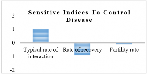
Sensitivity analysis helps pinpoint the factors contributing to variability in the model's hyperparameters, thus explaining differences in model results [5, 12]. It serves multiple purposes: identifying key input variables that have the most significant impact on the model's outcome, allowing for prioritization of these variables and reduction of simulation time; assessing the influence of relationships between input parameters; and discovering potential model simplifications. In our context, sensitivity analysis can determine the significance of each parameter in relation to disease spread, enabling us to focus on the variables that most significantly affect the basic reproduction number, $R_0$, and direct our intervention efforts accordingly. The normalized forward sensitive analysis is calculated by the formula $Y_p^{R_0}=\frac{\partial R_0}{\partial p} \times \frac{p}{\left|R_0\right|}$ where $p$ is the parameter in basic reproduction number. The sensitive indices for our model are shown in Figure 1.
Figure 1. Sensitive indices to control disease
$\begin{gathered}\frac{\partial R_0}{\partial \beta} \times \frac{\beta}{\left|R_0\right|}=+1 \\ \frac{\partial R_0}{\partial \gamma} \times \frac{\gamma}{\left|R_0\right|}=-0.9107 \\ \frac{\partial R_0}{\partial \pi} \times \frac{\pi}{\left|R_0\right|}=-0.08929\end{gathered}$
In SIR mathematical model, the bifurcation parameter is often related to basic reproduction number, which is a key determinant of disease transmission dynamics.it is a dimensionless number that integrates various biological environment and behavioural factors affecting the spread of infectious disease. The bifurcation parameter of our model is found to be $\beta^*=\frac{\gamma+\pi}{1-p}$.
5.1 Transcritical bifurcation
In the context of the basic SIR model used in epidemiology to describe the spread of infectious diseases, a transcritical bifurcation refers to a type of critical point where the stability of the disease-free equilibrium (DFE) and the endemic equilibrium swap as a parameter crosses a critical value.
Let us consider the set of equations Let us consider the set of equations $\frac{d S}{d t}=(1-\mathrm{p}) \pi-\beta \mathrm{SI}- \pi S$:
$\frac{d I}{d t}=\beta S I-(\gamma+\pi) I ; \frac{d R}{d t}=p \pi+\gamma I-\pi R$
The Jacobian of the above equation is found as
$J=\left[\begin{array}{ccc}-\beta \mathrm{I}-\pi & -\beta \mathrm{S} & 0 \\ \beta \mathrm{I} & \beta \mathrm{S}-(\gamma+\pi) & 0 \\ 0 & \gamma & -\pi\end{array}\right]$
Now we find the Jacobian at $\left(M_0, \beta^*\right)$
$J_{\left(M_0, \beta^*\right)}=\left[\begin{array}{ccc}-\pi & -\beta^*(1-\mathrm{p}) & 0 \\ 0 & 0 & 0 \\ 0 & \gamma & -\pi\end{array}\right]$
The characteristic equation is given by $|J-\lambda I|=0$
$\left|\begin{array}{ccc}-\pi-\lambda & -\beta^*(1-\mathrm{p}) & 0 \\ 0 & -\lambda & 0 \\ 0 & \gamma & -\pi-\lambda\end{array}\right|=0$
$(-\pi-\lambda)(-\lambda)(-\pi-\lambda)=0$
The eigen values are $0,-0.2,-0.2$.
Since it has one zero eigen value and 2 negative eigen value, hence our model does not have saddle point.
We can proceed further, let $\lambda_1=0, \lambda_2=\lambda_3=-0.2$, now we find the eigen vector $X=\left(x_1, x_2, x_3\right)^T$ corresponding to $\lambda_1$ which satisfy $J X=\lambda_1 X$.
$\left[\begin{array}{ccc}-\pi & -\beta^*(1-p) & 0 \\ 0 & 0 & 0 \\ 0 & \gamma & -\pi\end{array}\right]\left[\begin{array}{l}x_1 \\ x_2 \\ x_3\end{array}\right]=0$
$\begin{gathered}-\pi x_1-\beta^*(1-\mathrm{p}) x_2=0 \\ \gamma x_2-\pi x_3=0\end{gathered}$
Solving the above equations, we get $\pi x_1=-\beta^*(1-\mathrm{p}) x_2$.
Thus $x_1=\frac{-\beta^*(1-\mathrm{p})}{\pi} x_2$.
Also, $x_3=\frac{\gamma}{\pi} x_2$.
Let $A_1=\frac{-\beta^*(1-\mathrm{p})}{\pi}$ and $A_2=\frac{\gamma}{\pi}$.
Hence $x_1=A_1 x_2$ and $x_3=A_2 x_2$.
Thus $X=\left(\begin{array}{c}A_1 x_2 \\ x_2 \\ A_2 x_2\end{array}\right)$.
Now we find the eigen vector $Y=\left(y_1, y_2, y_3\right)^T$. corresponding to $\lambda_1$ which satisfy $J^T Y=\lambda_1 Y$.
$\left[\begin{array}{ccc}-\pi & 0 & 0 \\ -\beta^*(1-\mathrm{p}) & 0 & \gamma \\ 0 & 0 & -\pi\end{array}\right]\left[\begin{array}{l}y_1 \\ y_2 \\ y_3\end{array}\right]=0$
$-\pi y_1=0,-\beta^*(1-\mathrm{p}) y_1+\gamma y_3=0,-\pi y_3=0$
Solving the above equations, we get
$y_1=y_3=0 ; Y=\left(\begin{array}{c}0 \\ y_2 \\ 0\end{array}\right)$
Now we write system of equations in equations in the vector form as $\frac{d Y}{d t}=g(x)$, where
$Y=(S, I, R)^T ; g=\left(g_1, g_2, g_3\right)^T$
Now to calculate $\frac{d g}{d \beta}=g_\beta$.
$\begin{aligned} & \text { Let } g_1=(1-p) \pi-\beta S I-\pi S ; g_2=\beta S I-(\gamma+\pi) I ; g_3 = p \pi+\gamma I-\pi R ; \frac{d g_1}{d \beta}=-S I ; \frac{d g_2}{d \beta}=-S I ; \frac{d g_3}{d \beta}=0 ;g_\beta\left(M_0, \beta^*\right)=\left(\begin{array}{l}0 \\ 0 \\ 0\end{array}\right) .\end{aligned}$
Second condition to proceed Sotomayor theorem is also verified.
Now to check $Y^T\left[D g_\beta\left(M_0, \beta^*\right)\right] X \neq 0$,
$D g_\beta\left(M_0, \beta^*\right)=\left[\begin{array}{ccc}0 & -(1-\mathrm{p}) & 0 \\ 0 & 1-\mathrm{p} & 0 \\ 0 & 0 & 0\end{array}\right]$
Now,
$\begin{aligned} Y^T\left[D g_\beta\left(M_0, \beta^*\right)\right] X & =\left(y_1, y_2, y_3\right)\left[\begin{array}{ccc}0 & -(1-\mathrm{p}) & 0 \\ 0 & 1-\mathrm{p} & 0 \\ 0 & 0 & 0\end{array}\right]\left[\begin{array}{l}x_1 \\ x_2 \\ x_3\end{array}\right] = (1-p) x_2 y_2 \neq 0\end{aligned}$
According to Sotomayor theorem, when the parameter $\beta$ passing through $\beta^*$ then transcritical bifurcation occurs at measles free equilibrium point.
Damaturu is a Local Government Area (LGA) and the capital city of Yobe State in northern Nigeria. It is the headquarters of the Emirate. The Local Government Area has an area of 2,366 km2 and a population of 88,014 at the 2006 census. The Ministry’s Permanent Secretary, Isa Bukar, disclosed this, while briefing the State Deputy Governor, Idi Barde Gubana, who visited the State Specialist Hospital, Potiskum. A total of 836 suspected cases were reported from entire 17 LGAs of Yobe state with eight deaths; giving a CFR of 1.0%. Damaturu LGA accounted for the highest proportion 179(21.4%); also, more males 449 (53.7%) than females 387 (46.3%) were affected. About 727 (87%) of affected persons had not received any dose of Measles vaccine. Children 15 years or less accounted for 811 (97%) of all the cases. After giving vaccination by government in Yobe State Specialist Hospital, Continuous screening was done along with cluster mapping.
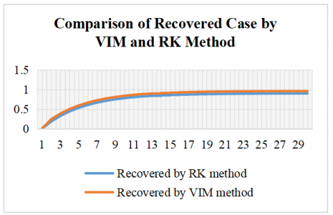
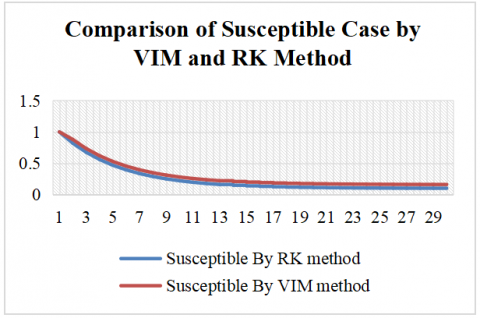
Numerical simulation is carried out by Variational Iteration Method (VIM) and Runge-Kutta (RK) methods: The initial conditions are S(0) = 1, I(0) = 0 and R(0) = 0.
The comparison between the RK and VIM for the SIR model reveals consistent differences in the estimated dynamics of the susceptible and recovered populations over a 30-day period are shown in Figures 2 and 3. With identical initial conditions (S(0) = 1, I(0) = 0, R(0) = 0), the RK method yields a faster decline in the susceptible population and a slower increase in the recovered population compared to VIM. Throughout the simulation, VIM consistently predicts higher values for the susceptible class and more rapid accumulation in the recovered class, indicating a relatively accelerated disease resolution.
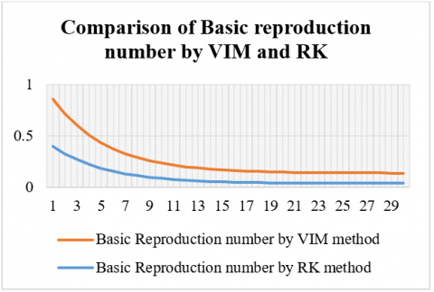
Figure 3. Comparison of basic reproduction number by VIM and RK
Table 2. Comparison of susceptible case by VIM and RK method
|
Days |
Susceptible By RK Method |
Susceptible By VIM Method |
|
1 |
1 |
1 |
|
2 |
0.82 |
0.88 |
|
3 |
0.676 |
0.736 |
|
4 |
0.5608 |
0.6208 |
|
5 |
0.46864 |
0.52864 |
|
6 |
0.394912 |
0.454912 |
|
7 |
0.3359296 |
0.3959296 |
|
8 |
0.28874368 |
0.34874368 |
|
9 |
0.250994944 |
0.310994944 |
|
10 |
0.220795955 |
0.280795955 |
|
11 |
0.196636764 |
0.256636764 |
|
12 |
0.177309411 |
0.237309411 |
|
13 |
0.161847529 |
0.221847529 |
|
14 |
0.149478023 |
0.209478023 |
|
15 |
0.139582419 |
0.199582419 |
|
16 |
0.131665935 |
0.191665935 |
|
17 |
0.125332748 |
0.185332748 |
|
18 |
0.120266198 |
0.180266198 |
|
19 |
0.116212959 |
0.176212959 |
|
20 |
0.112970367 |
0.172970367 |
|
21 |
0.110376294 |
0.170376294 |
|
22 |
0.108301035 |
0.168301035 |
|
23 |
0.106640828 |
0.166640828 |
|
24 |
0.105312662 |
0.165312662 |
|
25 |
0.10425013 |
0.16425013 |
|
26 |
0.103400104 |
0.163400104 |
|
27 |
0.102720083 |
0.162720083 |
|
28 |
0.102176066 |
0.162176066 |
|
29 |
0.101740853 |
0.161740853 |
|
30 |
0.101392683 |
0.161392683 |
Table 3. Comparison of recovered case by VIM and RK method
|
Recovered by RK Method |
Recovered by VIM Method |
|
0 |
0 |
|
0.18 |
0.24 |
|
0.324 |
0.384 |
|
0.4392 |
0.4992 |
|
0.53136 |
0.59136 |
|
0.605088 |
0.665088 |
|
0.6640704 |
0.7240704 |
|
0.71125632 |
0.77125632 |
|
0.749005056 |
0.809005056 |
|
0.779204045 |
0.839204045 |
|
0.803363236 |
0.863363236 |
|
0.822690589 |
0.882690589 |
|
0.838152471 |
0.898152471 |
|
0.850521977 |
0.910521977 |
|
0.860417581 |
0.920417581 |
|
0.868334065 |
0.928334065 |
|
0.874667252 |
0.934667252 |
|
0.879733802 |
0.939733802 |
|
0.883787041 |
0.943787041 |
|
0.887029633 |
0.947029633 |
|
0.889623706 |
0.949623706 |
|
0.891698965 |
0.951698965 |
|
0.893359172 |
0.953359172 |
|
0.894687338 |
0.954687338 |
|
0.89574987 |
0.95574987 |
|
0.896599896 |
0.956599896 |
|
0.897279917 |
0.957279917 |
|
0.897823934 |
0.957823934 |
|
0.898259147 |
0.958259147 |
|
0.898607317 |
0.958607317 |
Table 4. Comparison of basic reproduction number by VIM and RK
|
Basic Reproduction Number by RK Method |
Basic Reproduction Number by VIM Method |
|
0.401785714 |
0.461785714 |
|
0.329464286 |
0.389464286 |
|
0.271607143 |
0.331607143 |
|
0.225321429 |
0.285321429 |
|
0.188292857 |
0.248292857 |
|
0.15867 |
0.21867 |
|
0.134971714 |
0.194971714 |
|
0.116013086 |
0.176013086 |
|
0.100846183 |
0.160846183 |
|
0.088712661 |
0.148712661 |
|
0.079005843 |
0.139005843 |
|
0.071240388 |
0.131240388 |
|
0.065028025 |
0.125028025 |
|
0.060058134 |
0.120058134 |
|
0.056082222 |
0.116082222 |
|
0.052901492 |
0.112901492 |
|
0.050356908 |
0.110356908 |
|
0.04832124 |
0.10832124 |
|
0.046692707 |
0.106692707 |
|
0.04538988 |
0.10538988 |
|
0.044347618 |
0.104347618 |
|
0.043513809 |
0.103513809 |
|
0.042846761 |
0.102846761 |
|
0.042313123 |
0.102313123 |
|
0.041886213 |
0.101886213 |
|
0.041544685 |
0.101544685 |
|
0.041271462 |
0.101271462 |
|
0.041052884 |
0.101052884 |
|
0.040878021 |
0.100878021 |
|
0.040738131 |
0.100738131 |
Additionally, the basic reproduction number (R₀) obtained through both methods demonstrates a decreasing trend over time; however, values obtained via VIM are marginally higher than those from RK at each step, suggesting a slightly slower perceived reduction in transmission under VIM. These discrepancies highlight the influence of numerical technique on the simulation outcomes and suggest that VIM may offer a more conservative estimate of disease spread dynamics. Both methods effectively replicate the qualitative behavior of the epidemic, yet the variation in their outputs underscores the importance of method selection in epidemiological modeling. Simulations further show that increasing vaccination coverage significantly alters the trajectory of measles transmission. At low coverage levels, the model predicts large outbreaks, while increasing vaccination rates toward the critical threshold leads to a sharp decline in infection levels. At the critical vaccination threshold, the system exhibits a transcritical bifurcation, where the disease-free equilibrium becomes stable and the endemic equilibrium vanishes. For a basic reproduction number of 10, the estimated critical vaccination coverage is 90%, and simulations near this threshold show that even slight deviations (89.9%) can result in minor outbreaks. This demonstrates the importance of maintaining high vaccination coverage to eliminate disease persistence and prevent resurgence, emphasizing the sensitivity of measles control to precise vaccination rates (Tables 2-4).
This study developed and analyzed a mathematical model for measles transmission using the classical SIR framework, incorporating a vaccination term to evaluate the impact of immunization strategies on disease dynamics. Both analytical methods and numerical simulations were employed, including a comparative study using the RK and VIM. The results revealed consistent variations between the two numerical approaches. The RK method showed a more rapid decline in the susceptible population and a slower rise in the recovered population, while the VIM method produced slightly higher values for both susceptible and recovered classes, indicating a relatively accelerated disease resolution. Additionally, the basic reproduction number (R₀), which showed a declining trend in both methods, remained consistently higher under VIM, suggesting a more conservative projection of disease persistence. These differences emphasize the influence of numerical method selection on simulation outcomes and the interpretation of epidemiological dynamics. Quantitatively, the analysis confirmed that for a basic reproduction number of 10, at least 90% vaccination coverage is required to eliminate the disease. Simulations demonstrated that even marginal deviations from this threshold—such as a drop to 89.9%—can result in small but nontrivial outbreaks, affecting approximately 0.10% of the population. This behavior aligns with the predicted forward (transcritical) bifurcation, wherein the disease-free equilibrium becomes stable and the endemic state disappears once the critical vaccination threshold is surpassed. The narrow margin between control and resurgence underscores the necessity of sustaining high vaccination rates. While the model captures essential aspects of measles transmission, it operates under simplifying assumptions, including homogeneous mixing, perfect vaccine efficacy, and constant population size. These assumptions, though useful for analytical tractability, limit the applicability of the model in more complex real-world scenarios where factors such as age structure, spatial distribution, or waning immunity may significantly influence outcomes. Future work should address these limitations by extending the model to incorporate heterogeneities, stochastic effects, and spatial or age-structured compartments.
[1] Agusto, F.B. (2017). Mathematical model of Ebola transmission dynamics with relapse and reinfection. Mathematical Biosciences, 283: 48-59. https://doi.org/10.1016/j.mbs.2016.11.002
[2] Althaus, C.L., Low, N., Musa, E.O., Shuaib, F., Gsteiger, S. (2015). Ebola virus disease outbreak in Nigeria: Transmission dynamics and rapid control. Epidemics, 11: 80-84. https://doi.org/10.1016/j.epidem.2015.03.001
[3] Chowell, G., Nishiura, H. (2014). Transmission dynamics and control of Ebola virus disease: A review. BMC Medicine, 12: 1-16. https://doi.org/10.1186/s12916-014-0196-0
[4] D’Silva, J.P., Eisenberg, M.C. (2017). Modelling spatial invasion of Ebola in West Africa. Journal of Theoretical Biology, 428: 65-75. https://doi.org/10.1016/j.jtbi.2017.05.034
[5] Li, L. (2017). Transmission dynamics of Ebola virus disease with human mobility in Sierra Leone. Chaos. Solitons and Fractals, 104: 575-579. https://doi.org/10.1016/j.chaos.2017.09.022
[6] Njankou, S.D.D., Nyabadza, F. (2016). An optimal control model for Ebola virus disease. Journal of Biological Systems, 24(1): 29-49. https://doi.org/10.1142/S0218339016500029
[7] Rachab, A., Torres, D.F.M. (2014). Mathematical modeling, simulation and optimal control of the 2014 Ebola outbreak in West Africa. Discrete Dynamics in Nature and Society, 2015(1): 842792. https://doi.org/10.1155/2015/842792
[8] Dia, P., Constantine, P., Kalmbach, K., Jones, E., Pankavich, S. (2018). A modified SEIR model for the spread of Ebola in Western Africa and metrics for resource allocation. Applied Mathematics and Computation, 324: 141-155. https://doi.org/10.1016/j.amc.2017.11.039
[9] Sedelnikov, A.V. (2018). Mean of microaccelerations estimate in the small spacecraft internal environment with the use of fuzzy sets. Microgravity Science and Technology, 30: 503-509. https://doi.org/10.1007/s12217-018-9620-y
[10] Coltart, C.E., Lindsey, B., Ghinai, I., Johnson, A.M., Heymann, D.L. (2017). The Ebola outbreak, 2013-2016: Old lessons for new epidemics. Philosophical Transactions of the Royal Society B, 372: 20160297. https://doi.org/10.1098/rstb.2016.0297
[11] Barros, L.C.D.E., Leite, M.B.F., Bassanezi, R.C. (2003). The SI epidemiological models with a fuzzy transmission parameter. Computers & Mathematics with Applications, 45(10-11): 1619-1628. https://doi.org/10.1016/S0898-1221(03)00141-X
[12] Farahi, M.H., Barati, S. (2011). Fuzzy time-delay dynamical systems. Journal of Mathematics and Computer Science, 2(1): 44-53. https://doi.org/10.22436/jmcs.002.01.06
[13] Das, A., Pal, M. (2018). A mathematical study of an imprecise SIR epidemic model with treatment control. Journal of Applied Mathematics and Computing, 56: 477-500. https://doi.org/10.1007/s12190-017-1083-6
[14] Verma, R., Tiwari, S.P., Upadhyay, R.K. (2018). Fuzzy modeling for the spread of influenza virus and its possible control. Computational Ecology and Software, 8(1): 32-45.
[15] Sadhukhan, D., Sahoo, L.N., Mondal, B., Maitri, M. (2010). Food chain model with optimal harvesting in fuzzy environment. Journal of Applied Mathematics and Computing, 34: 1-18. https://doi.org/10.1007/s12190-009-0301-2
[16] Bhavithra, H.A., Sindu Devi, S. (2024). Feasibility and stability analysis for basic measles model using fuzzy parameter. Contemporary Mathematics, 5(1): 897-912. https://doi.org/10.37256/cm.5120242428
[17] Bhavithra, H.A., Sindu Devi, S. (2024). Sensitivity stability and feasibility analysis of epidemic Measles using mathematical SEIR model. OPSEARCH, 61: 1-30. https://doi.org/10.1007/s12597-024-00848-z
[18] Sedelnikov, A.V., Safronov. S.L, Khnyreva, E.S. (2019). Control of rotational motion of a partially inoperable small spacecraft using fuzzy sets. Journal of Physics: Conference Series, 1260: 032035. https://doi.org/10.1088/1742-6596/1260/3/032035
[19] Ahmad, I., Ali, Z., Khan, B., Shah, K., Abdeljawad, T. (2025). Exploring the dynamics of Gumboro-Salmonella co-infection with fractal fractional analysis. Alexandria Engineering Journal, 117: 472-489 https://doi.org/10.1016/j.aej.2024.12.119
[20] Yadav, A.K., Basavegowda, N., Shirin, S., Raju, S., Sekar, R., Somu, P., Uthappa, U.T., Abdi, G. (2025). Emerging trends of gold nanostructures for point-of-care biosensor-based detection of COVID-19. Molecular Biotechnology, 67: 1398-1422. https://doi.org/10.1007/s12033-024-01157-y
[21] Gurjar, S.P., Roy, A., Gupta, A., Khatana, K., Kumar, A., Raja, V., Raj, S., Verma, D. (2025). Computational studies of amla (Phyllanthus emblica) bioactive compounds against COVID-19 mutants (PDB ID: 7T9L and 7V8B). Letter in Applied NanoBioScience, 14(2): 1-11. https://doi.org/10.33263/LIANBS142.089
[22] Dwivedi, A., Keval, R., Baniya, V. (2022). A mathematical study of dynamical model for Japanese encephalitis-dengue co-infection using JE vaccine. International Journal of Mathematical Modelling and Numerical Optimisation, 12(4): 416-442. https://doi.org/10.1504/IJMMNO.2022.126564
[23] Bhavithra, H.A., Sindhuja, S., Ramalingam, N., Devi, S.S. (2025). Forward-backward transcritical bifurcation: Control and optimisation in a novel fuzzy SIR model. International Journal of Mathematical Modelling and Numerical Optimisation, 15(3): 246-269. https://doi.org/10.1504/IJMMNO.2025.147576