Abderrazek Menasri*![]() | Ahmed Seddiki
| Ahmed Seddiki![]()
© 2025 The authors. This article is published by IIETA and is licensed under the CC BY 4.0 license (http://creativecommons.org/licenses/by/4.0/).
OPEN ACCESS
This study employs an Autoregressive Moving Average (ARMA) statistical model to generate artificial seismograms, an innovative approach to address the lack of real-world data. The model is driven by white Gaussian noise and modulated by an amplitude envelope function, allowing it to faithfully reproduce the characteristics of seismic motion. This model proved particularly effective in simulating the non-stationary behavior of accelerograms from historical earthquakes in Algeria, including those in Boumerdès, Asnam, and Affroun. A comparative analysis of key parameters such as peak acceleration and shaking duration confirmed the validity of the simulations. Beyond simple reproduction, the generated seismograms made it possible to assess damage potential. The researchers measured crucial structural demand indicators, such as ductility demand and hysteretic energy, to assess potential damage. The response spectra of the simulations match well with those of the real recordings, which reinforces the reliability of the damage predictions. The quasi-linear correlation between the damage index and the initial structural period reinforces this observation. In summary, the ARMA(2,1) approach offers a practical and reliable framework for damage assessment and the design of earthquake-resistant structures.
Autoregressive Moving Average (ARMA) statistical model, simulation, ductility, hysteretic energy, response spectra, damage
The limited availability and inherent variability of natural accelerogram records often hinder a full analysis of structural response. Consequently, the generation of artificial ground motions has become an essential and widely accepted practice in earthquake engineering. These simulated accelerograms allow for a systematic evaluation of structures under both linear and nonlinear conditions, offering enhanced control over crucial parameters such as amplitude, duration, and frequency content. Response spectra play a central role in seismic design, particularly for single-degree-of-freedom (SDOF) systems [1]. When multiple records are used to develop design spectra, a significant degree of variability emerges [2]. To address this, records are frequently normalized with respect to peak parameters, such as acceleration or velocity [3]. This approach has been widely used, for example, in the seismic design of nuclear power plants [4].
This study aims to develop minimal stochastic models for earthquake ground motions to address these shortcomings. The objective is to create a simple yet descriptive modeling method that captures the damage-relevant characteristics of seismic input. To achieve this, we propose using a time-varying Auto Regressive Moving Average (ARMA) process, specifically a low-order ARMA(2,1) model. This model is driven by white noise and modulated by an envelope function, which allows it to effectively reproduce the non-stationary behavior of seismic events.
The methodology, applied to Algerian earthquakes recorded on dense soils, confirmed that the model generates ground motions closely matching actual seismic records. The study's results demonstrate that the model can accurately predict the mean values and variances of key spectral response ordinates. The simulations show a good correspondence for key damage indicators, including peak displacement, ductility demand, and hysteretic energy dissipation. These findings confirm the validity of our approach as a valuable tool for assessing damage potential in seismic design applications.
This study analyzes seismic ground motion in the time domain using ARMA models, a method initially introduced by Jebb and Tay [5], and later adapted for structural dynamics by Gao et al. [6]. The ARMA framework was chosen for its ability to create simplified stochastic models that accurately capture ground motion characteristics while maintaining a clear physical interpretation. This interpretability is highly beneficial for structural design, as it allows a direct correlation between model parameters and measurable quantities like acceleration or displacement.
The ARMA model at any time step, $k$, is represented by the following equation:
$\begin{aligned} & A_k-\varphi_1 A_{k-1}-\cdots-\varphi_p A_{k-p} = W_k-\theta_1 A_{k-1}-\cdots-\theta_p W_{k-p}\end{aligned}$ (1)
where, $\phi_i$, $\theta_j$ are constant coefficients.
The left-hand side of this equation is the autoregressive (AR) part of order $p$, while the right-hand side is the moving average (MA) part of order $q$. In this context, $Z_t$ represents the time series of measured data, and the sequence $a_t$ is a set of independent, identically distributed Gaussian random variables.
The constant coefficients, $\varphi_i$ and $\theta_j$, along with the model orders (p, q), are estimated from the data using a maximum likelihood approach. The seismic accelerograms from Table 1 were selected for this study.
Table 1. Real earthquakes characteristic
|
Event |
Boumerdes |
Asnam |
Affroun |
|
Magnitude |
6.8 |
5.8 |
6.8 |
|
Duration (second) |
25.96 |
21.7 |
80 |
|
Max Acceleration × (g) |
0.215 |
0.189 |
0.03 |
|
Number of points |
1299 |
1087 |
16001 |
In this research, the modeling process begins by normalizing the digitized seismic acceleration data to simplify the fitting of the model. For each time step, k, a moving window of 100 time steps centered at k is used to compute the root mean square Sk value.
This process generates a normalized time series, Zk = Ak/Sk, with a zero mean and unit variance. This series is then modeled as a second-order stationary process using the ARMA formulation Eq. (1).
The comprehensive procedure for fitting an ARMA model to a seismic acceleration record includes the following steps:
Normalization: Compute the experimental envelope function Sk and use it to normalize the raw acceleration data.
Envelope function: Define an analytical expression for Sk and estimate its parameters through least-squares analysis.
Stabilization: Remove any non-stationary trends from the original record using the envelope function to stabilize the signal.
Correlation analysis: Compute the autocorrelation and partial autocorrelation functions of the stabilized, normalized signal.
Order selection: Choose the appropriate order p for the AR component and order q for the MA component of the ARMA model (Eq. (1)).
Coefficient estimation: Estimate the coefficients φi and θj using maximum likelihood analysis.
Model validation: Validate the model by re-computing the autocorrelation and partial autocorrelation functions of the residuals to confirm that the selected orders are adequate and that the process is stationary.
Alternative model evaluation: Use the Akaike Information Criterion (AIC), denoted as AIC(p, q), to evaluate alternative model orders and select the one that minimizes the AIC value [7].
3.1 ARMA model and its parameters
From a parameter count perspective, the ARMA model offers a more efficient representation for simulating earthquake phenomena, particularly when data is affected by noise. A crucial step in evaluating ARMA parameters is analyzing the autocorrelation of the seismic trace. The relationship between autocorrelation and AR parameters highlights the primary importance of the AR part of the model as follows Eq. (4).
$\left[\begin{array}{cccc}1 & R_1 & \cdots & R_{k-1} \\ R_1 & \cdots & \cdots & R_{k-2} \\ \vdots & \cdots & \ddots & \vdots \\ R_{k-1} & 1 & \cdots & 1\end{array}\right]\left[\begin{array}{c}\emptyset_1 \\ \emptyset_2 \\ \vdots \\ \emptyset_k\end{array}\right]=\left[\begin{array}{c}R_1 \\ R_2 \\ \vdots \\ R_k\end{array}\right]$ (2)
Once the AR component is identified, the MA part can be constructed. For selecting the order of the ARMA(p, q) model, the minimum of the Akaike Information Criterion (AIC) is used, as investigated by Korte et al. [8]. For this purpose, the minimum of the AIC index:
$AIC\left( p,q \right)=N.ln\left( \sigma _{a}^{2} \right)+2\left( p+q \right)$ (3)
where, N is the sample size, and σa2 is the estimated variance from the residual maximum likelihood.
A comparison between several models for each earthquake: ARMA(1,1), ARMA(1,2), ARMA(2,1) and ARMA(2,2), using the AIC criterion described in Table 2.
Table 2. Application of AIC criteria to the different models
|
Parameter |
ARMA Model |
|||
|
(1,1) |
(1,2) |
(2,1) |
(2,2) |
|
|
Asnam |
-1145.4 |
-1157.9 |
-1158.3* |
-1155.0 |
|
Boumerdes |
-1170.3 |
-1185.5 |
-1190.2* |
-1186.5 |
|
Affroun |
-3.64068 |
-4.78432 |
-5.09023 |
-5.26325* |
* Indicates that the model has the minimum AIC.
The final model parameters for each earthquake are presented in Table 3.
Table 3. Parameters of the selected model
|
Parameter |
AR(1) |
AR(2) |
MA(1) |
σa |
|
Asnam |
0.359 |
-0.222 |
0.181 |
0.559 |
|
Boumerdes |
0.359 |
-0.869 |
-0.304 |
0.551 |
|
Affroun |
1.80244 |
-0.888599 |
-0.888599 |
-0.888599 |
This research selects an ARMA(2,1) model, which provided the best fit for the input accelerograms. This model can be represented by:
${{A}_{k}}-{{\varphi }_{1}}{{A}_{k-1}}-{{\varphi }_{2}}{{A}_{k-2}}={{W}_{k}}-{{\theta }_{1}}{{W}_{k-1}}$ (4)
For the simulation, the envelope function is given by the expression:
${{S}_{k}}=a.{{t}^{b}}.{{e}^{-ck}}$ (5)
The parameters a, b, and c are estimated through nonlinear regression analysis (Table 4).
The foundational assumption of this analysis is that an earthquake can be considered a single realization from a population of earthquakes characterized by an ARMA process.
Table 4. The parameters of the envelope function
|
Event |
Envelope Function Parameters |
||
|
A |
B |
C |
|
|
Boumerdes |
1.2198 |
1.1077 |
0.671 |
|
Asnam |
1.1567 |
0.8810 |
0.689 |
|
Affroun |
9.61e-9 |
10.91 |
0.6055 |
To simulate the acceleration time series using this approach, we first generate a white noise signal with a zero mean and a variance equal to the estimated variance. This white noise is then used as input to the ARMA model to produce a stationary time series. Finally, this stationary series is multiplied by the envelope function, S(k), to obtain the non-stationary simulated acceleration series.
Since the ARMA model is a linear combination of previous values and Gaussian random variables, simulated earthquakes can be generated inductively. For the ARMA(2,1) model, the recursive equation is used. To initiate the calculations, the first p values of Ak (in this case, A0 and A−1) are assumed to be zero. Gaussian random variables (Wk) with variance σa2 are generated as the white noise input.
Early simulations indicated that the Fourier spectra and responses derived from the simulated earthquakes had large values at low frequencies, which the original filtered earthquakes did not exhibit. This common issue is addressed by applying a low-pass filter to the simulated data to eliminate these low-frequency components.
The ARMA coefficients and the white noise standard deviation (σw) are detailed in Table 5.
Table 5. ARMA coefficients and white noise standard deviation
|
Event |
ARMA Parameters |
|||
|
$\phi_1$ |
$\phi_2$ |
$\phi_3$ |
$\sigma_{\mathrm{W}}$ |
|
|
Boumerdes |
0.6626 |
-0.0738 |
-0.521 |
0.555 |
|
Asnam |
0.4244 |
0.2411 |
-0.613 |
0.560 |
|
Affroun |
1.8635 |
-0.922845 |
-1.28836 |
0.0407843 |
For the estimator used, we provide the SSE, R-squared, adjusted R-squared, and RMSE in Table 6.
Table 6. Summary of fit metrics for the envelope function
|
Event |
SSE |
R² |
Adjusted R² |
RMSE |
|
Affroun |
2.674e + 04 |
0.6978 |
0.6978 |
1.293 |
A comparison of the key characteristics of real and simulated earthquakes (Table 7) shows that the events are well-characterized by the ARMA(2,1) process and the defined envelope function parameters.
Table 7. Characteristics earthquakes and simulated ones
|
Header |
Earthquakes |
|||
|
Characteristics |
Boumerdes |
Asnam |
Affroun |
|
|
Real |
Maximal acceleration × (g) |
0.152 |
0.189 |
0.030 |
|
Duration (sec) |
25.96 |
21.7 |
80 |
|
|
Simulated |
Maximal acceleration × (g) |
0.141 |
0.107 |
0.022 |
|
Duration (sec) |
20 |
20 |
80 |
|
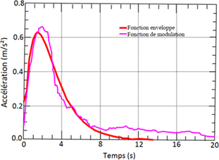
Figure 1. Modulation functions and envelope Boumerdes
Figure 2. Modulation functions and envelope Asnam
Figure 3. Modulation functions and envelope Affroun
Figures 1-3 show the appearance of the modulation functions and envelope functions corresponding to the Boumerdes, Asnam and Affroun earthquakes.
A range of damage measures has been developed to quantify the effects of seismic excitation on both linear and nonlinear structural systems [9-13]. Researchers have explored diverse approaches, as highlighted by Grigoriu's comparative evaluation [14]. While frequency spectra are a common way to present structural response data, any single measure is acknowledged to be an imperfect predictor of damage due to the variety of potential failure modes. Consequently, this study evaluates damage potential using a set of general and composite criteria, referred to as damage indices.
One such index, proposed by Park [15] is based on the ratio of structural demand to capacity. This index is a linear combination of the maximum relative deformation and the relative energy dissipation. The general form of the Park-Ang damage index is the frequency, damping and the yield force of a structure.
$DI=\frac{{{U}_{max}}\left( t \right)}{{{U}_{max}}}+\frac{\beta .\left[ {{E}_{H}} \right]}{{{R}_{Y}}.{{U}_{max}}}$ (6)
where, Umax(t) is the maximum displacement under seismic loading. Uu is the ultimate deformation capacity under monotonic loading. RY is the yield force. EH is the hysteretic energy dissipated through inelastic deformation. β is a non-negative parameter that represents the structure's energy absorption capacity.
To calculate a spectrum of damage indices, it is necessary to specify the value of β and the structural parameters, including natural frequency, damping ratio, and yield force.
The structural responses (Umax(t)) were calculated through numerical integration of the equations of motion, assuming a linear acceleration within each time step [16-21]. To accurately model the energy absorption of structures, a bilinear hysteretic model was adopted.
This model is defined by three key parameters:
uy: initial yield displacement,
k1: initial elastic stiffness,
ky: post-yield stiffness.
During monotonic loading, the restoring force R(u, t) follows:
R(u, t) = K1.u(t); u(t) ≤ uy (7)
R(u, t) = Ky.(u(t)-uz); u(t) > uy (8)
During unloading, the stiffness reverts to the initial elastic stiffness until the displacement again intersects the yield envelope. This elastoplastic behavior is captured by setting Ky = 0 and R(u, t) = Ky.uy for u(t) > uy.
This simplified yet effective model is widely used in seismic analysis to estimate damage potential.
The dataset for this study includes two recorded earthquake ground motions:
•The 2003 Boumerdes (NS) earthquake, with a moment magnitude M = 6.8, yielding 1299 data points at 0.02-second intervals.
•The 1980 Asnam (NE) earthquake, with a moment magnitude M = 5.8, providing 1087 data points at 0.02-second intervals.
•The 1988 Affroun earthquake, with a moment magnitude M = 6.8, yielding 1601 points.
Various ARMA models were fitted to these records. For each earthquake, 20 synthetic acceleration records were generated using the identified ARMA models. These synthetic records were then used as input for elastoplastic SDOF systems, which were modeled with a bilinear hysteresis law (Figure 4).
Figure 4. Response of SDOF system
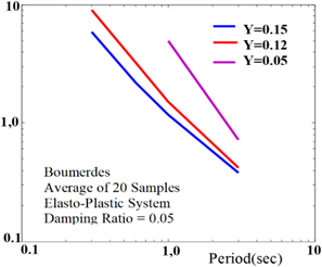
The analyses were performed with damping ratios of 0.02 and 0.05, and yield strength ratios (Y = RY/M⋅g) of 0.05, 0.10, and 0.15 to represent different levels of structural ductility. For the damage index calculations, the β parameter in the Park-Ang index was set to 0.05, which is a value reflecting the average energy dissipation capacity of typical steel structures.
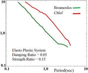
The resulting damage index spectra (Figures 5-7) were obtained by evaluating the Park-Ang index across a range of natural frequencies. These spectra are a combination of two fundamental response measures: the ductility demand spectrum and the hysteretic energy demand spectrum.
As shown in Figure 2, the damage index spectra for individual earthquakes display notable irregularities due to the inherent randomness of ground motion characteristics. This highlights the importance of using ensemble averages or statistically representative simulations for damage assessment.
Figure 5. Seismic damage spectra for the 1980 Asnam and 2003 Boumerdes events
Figure 6. Average spectral damage from synthetic motions for the 1980 Asnam and 2003 Boumerdes events
Figure 7. Average spectral damage vs strength reduction factor for the 2003 Boumerdes events
This study confirms that ARMA(2,1) time-domain models are a compact and effective tool for simulating earthquake ground motions. Despite the model’s simplicity, the simulated response spectra show good agreement with real records. However, some discrepancies were noted for long-period motions, likely due to residual low-frequency components from filtering. The envelope function successfully controls the amplitude and duration of the synthetic motions, which are key characteristics of seismic inputs.
The results also emphasize the significant influence of the soil behavior model on seismic response, underscoring the need to incorporate realistic, and potentially nonlinear, site effects into simulations. The ARMA(2,1) based approach therefore provides a practical framework for generating site-specific synthetic records for performance-based seismic design.
Furthermore, the irregularities in the damage index spectra of individual records appear to be the result of stochastic variability rather than intrinsic features of the seismic source. A nearly linear correlation was observed between the logarithm of the average damage index and the logarithm of the initial structural period. If validated with larger datasets, this trend could greatly improve the predictive power of structural damage models and lead to more accurate seismic hazard assessments. The observed decrease in the average damage index as the structural period increases supports the established understanding that long-period structures are generally less vulnerable.
In summary, these findings advocate for a combined approach using ARMA-based modeling and period-dependent damage assessment to develop next-generation, performance-oriented methodologies for earthquake-resistant design.
This work is supported by the Geomaterials Development Laboratory, Med Boudiaf University of M’sila, Algeria.
|
Zt |
time series of measured data |
|
at, Wk |
Gaussian random variables |
|
Sk |
root mean square value |
|
Zk |
normalized time series |
|
AIC |
Akaike Information Criterion |
|
N |
sample size |
|
a, b, c |
parameters of the envelope function |
|
S(k) |
envelope function |
|
DI |
damage index |
|
uy |
initial yield displacement |
|
k1 |
initial elastic stiffness |
|
ky |
post-yield stiffness |
|
SDOF |
single-degree-of-freedom |
|
$\phi$, Ɵ |
ARMA constant coefficients |
|
σa2 |
estimated variance |
|
σw |
standard deviation |
|
(p, q) |
model orders |
[1] Laseima, S.Y., Mutalib, A.A., Osman, S.A., Hamid, N.H. (2020). Seismic behavior of exterior RC beam-column joints retrofitted using CFRP sheets. Latin American Journal of Solids and Structures, 17(5): e263. https://doi.org/10.1590/1679-78255910
[2] Yaghmaei-Sabegh, S., Safari, S., Abdolmohammad-Ghayouri, K. (2019). Characterization of ductility and inelastic displacement demand in base-isolated structures considering cyclic degradation. Journal of Earthquake Engineering, 23(4): 557-591. https://doi.org/10.1080/13632469.2017.1326415
[3] Kubo, T., Yamamoto, T., Sato, K., Jimbo, M., Imaoka, T., Umeki, Y. (2014). A seismic design of nuclear reactor building structures applying seismic isolation system in a high seismicity region–A feasibility case study in Japan. Nuclear Engineering and Technology, 46(5): 581-594. https://doi.org/10.5516/NET.09.2014.716
[4] Yu, C.C., Whittaker, A.S. (2024). Generating seismic design basis spectra for us nuclear energy facilities. Nuclear Engineering and Design, 426: 113333. https://doi.org/10.1016/j.nucengdes.2024.113333
[5] Jebb, A.T., Tay, L. (2017). Introduction to time series analysis for organizational research: Methods for longitudinal analyses. Organizational Research Methods, 20(1): 61-94. https://doi.org/10.1177/1094428116668035
[6] Gao, Y., Mosalam, K.M., Chen, Y., Wang, W., Chen, Y. (2021). Auto-regressive integrated moving-average machine learning for damage identification of steel frames. Applied Sciences, 11(13): 6084. https://doi.org/10.3390/app11136084
[7] Vrieze, S.I. (2012). Model selection and psychological theory: A discussion of the differences between the Akaike information criterion (AIC) and the Bayesian information criterion (BIC). Psychological Methods, 17(2): 228. https://doi.org/10.1037/a0027127
[8] Korte, J., Brockmann, J.M., Schuh, W.D. (2023). A comparison between successive estimate of TVAR (1) and TVAR (2) and the estimate of a TVAR (3) process. Engineering Proceedings, 39(1): 90. https://doi.org/10.3390/engproc2023039090
[9] Sarwar, W., Sarwar, R. (2019). Vibration control devices for building structures and installation approach: A review. Civil and Environmental Engineering Reports, 29(2): 74-100. https://doi.org/10.2478/ceer-2019-0018
[10] Bao, Y., Becker, T.C. (2018). Inelastic response of base-isolated structures subjected to impact. Engineering Structures, 171: 86-93. https://doi.org/10.1016/j.engstruct.2018.05.091
[11] Gurbuz, T., Cengiz, A. (2025). Structural damages during the February 06, 2023 Kahramanmaraş earthquakes in Turkey. Soil Dynamics and Earthquake Engineering, 191: 109214. https://doi.org/10.1016/j.soildyn.2025.109214
[12] Zhu, L., Elwood, K.J., Haukaas, T. (2007). Classification and seismic safety evaluation of existing reinforced concrete columns. Journal of Structural Engineering, 133(9): 1316-1330. https://doi.org/10.1061/(ASCE)0733-9445(2007)133:9(1316)
[13] Giannini, R., Paolacci, F., Phan, H.N., Corritore, D., Quinci, G. (2022). A novel framework for seismic risk assessment of structures. Earthquake Engineering & Structural Dynamics, 51(14): 3416-3433. https://doi.org/10.1002/eqe.3729
[14] Aghababaei, M., Mahsuli, M. (2019). Component damage models for detailed seismic risk analysis using structural reliability methods. Structural Safety, 76: 108-122. https://doi.org/10.1016/j.strusafe.2018.08.004
[15] Park, R. (1989). Evaluation of ductility of structures and structural assemblages from laboratory testing. Bulletin of the New Zealand Society for Earthquake Engineering, 22(3): 155-166. https://doi.org/10.5459/bnzsee.22.3.155-166
[16] Nayfeh, A.H. (2024). Linear and Nonlinear Structural Mechanics. John Wiley & Sons. https://doi.org/10.1002/9783527617562
[17] Brahimi, M., Berri, S. (2006). The use of ARMA models in earthquake response spectra. International Conference on Nuclear Engineering, 42444: 7-13. https://doi.org/10.1115/ICONE14-89023
[18] Armanini, C., Dal Corso, F., Misseroni, D., Bigoni, D. (2019). Configurational forces and nonlinear structural dynamics. Journal of the Mechanics and Physics of Solids, 130: 82-100. https://doi.org/10.1016/j.jmps.2019.05.009
[19] Han, S., Bauchau, O.A. (2023). Configurational forces in variable-length beams for flexible multibody dynamics. Multibody System Dynamics, 58(3): 275-298. https://doi.org/10.1007/s11044-022-09866-5
[20] Lacarbonara, W. (2013). Nonlinear Structural Mechanics: Theory, Dynamical Phenomena and Modeling. Springer Science & Business Media. https://doi.org/10.1007/978-1-4419-1276-3
[21] Mallett, R.H., Marcal, P.V. (1968). Finite element analysis of nonlinear structures. Journal of the Structural Division, 94(9): 2081-2106. https://doi.org/10.1061/JSDEAG.0002066