Mohammed Dh. Al Arabo*![]() | Fikriye Yılmaz
| Fikriye Yılmaz![]()
© 2025 The authors. This article is published by IIETA and is licensed under the CC BY 4.0 license (http://creativecommons.org/licenses/by/4.0/).
OPEN ACCESS
Non-convex optimization continues to be a fundamental challenge in applied mathematics, engineering, and data science, with applications that encompass machine learning and image processing. Building on the recent Dilara, Ebru, and Ibrahim (DEI) conjugate gradient method (a conjugate gradient (CG) algorithm designed for non-convex problems), this paper proposes three novel hybrid CG algorithms—NEW1, NEW2, and NEW3—that aim to expedite convergence by adaptively updating the rule that forms each new search direction (often denoted as β) while maintaining theoretical guarantees of global convergence and sufficient descent. We provide detailed convergence proofs for each algorithm under standard assumptions. Comprehensive evaluations on 32 benchmark functions with varying dimensionality and conditioning show average reductions of up to 49% in the number of iterations (NOI) and up to 60% in the number of function (NOF) evaluations, compared to DEI. In practical terms, these gains translate into lower computational costs on challenging real-world problems (e.g., engineering design and machine learning optimization) without sacrificing robustness, positioning NEW1–NEW3 as efficient, theoretically grounded alternatives to conventional CG methods.
adaptive algorithms, benchmark functions, nonlinear conjugate gradient, sufficient descent, unconstrained optimization
Unconstrained nonlinear optimization is central to many scientific and engineering applications, from physics simulations to training machine learning models. Conjugate gradient (CG) methods remain popular for these problems because of their memory efficiency and ability to handle high-dimensional spaces [1, 2]. Yet on non-convex landscapes they may become unstable and slow to converge, motivating improvements to β update rules.
The Dilara, Ebru, and Ibrahim (DEI) algorithm, proposed by Akdag et al. [3], marked a substantial advancement by ensuring sufficient descent and global convergence for non-convex problems. Nevertheless, in empirical assessments, DEI sometimes necessitates numerous iterations and function evaluations, which may constrain its efficiency in large-scale applications. We build on DEI with adaptive β strategies that preserve sufficient descent and global convergence while targeting lower computational cost.
Our objective is to develop a CG family that retains DEI’s guarantees while mitigating β-sensitivity in non-convex settings, and to state the novelty explicitly via the following contributions:
• Proposal of three hybrid CG algorithms (NEW1–NEW3) with adaptive β updates for forming search directions.
• Theoretical guarantees: sufficient descent and global convergence under standard line-search assumptions.
• Empirical validation on 32 benchmarks showing up to 49% fewer number of iterations (NOI) and up to 60% fewer number of function (NOF) compared to DEI.
2.1 Classical conjugate gradient methods
Conjugate gradient methods were initially devised to efficiently address linear systems without the explicit formation of matrices [1]. Fletcher and Reeves [2] expanded their work to nonlinear optimization, leading to the development of methods such as Polak-Ribière-Polyak (PRP), along with variations PRP+, PRP-PR, and PRP-T, which are more responsive to the curvature of nonlinear objectives. Kou [4] advanced the discipline by providing an enhanced CG approach with optimal characteristics for general unconstrained optimization, emphasizing the potential of customizing conjugate gradient updates to the geometry of the problem. Compared to these classical schemes, our algorithms retain the CG framework but target non-convex robustness explicitly via adaptive β updates while keeping per-iteration cost comparable to standard CG.
2.2 Sufficient descent and convergence
Adequate descent conditions guarantee that the search direction results in significant objective reduction at each iteration. Gilbert and Nocedal [5], together with Dai and Yuan [6], formulated formal criteria that guarantee convergence for a wide range of nonlinear functions. The aforementioned conditions depend on characteristics such as bounded level sets and the Lipschitz continuity of the gradient. Our methods are designed to satisfy sufficient descent and global convergence under standard line-search assumptions, aligning with these criteria while enabling more aggressive search directions in non-convex regions.
2.3 DEI-related methods and extensions
Recent methodologies have enhanced β update rules by integrating restart conditions and regularization terms [7, 8]. The DEI algorithm developed by Akdag et al. [3] denotes a significant advancement, demonstrating sufficient descent and global convergence through the strategic implementation of the β_DEI parameter. Nonetheless, the conservative updates of DEI frequently lead to elevated NOI and NOF, causing the formulation of more aggressive yet stable hybrid strategies. Building directly on DEI, our approach adapts β using local curvature cues while preserving DEI’s descent and convergence guarantees, thereby reducing function/gradient calls in practice.
Recent research has advanced Dai–Yuan-type and spectral conjugate gradient methods with sufficient descent properties, directly addressing the challenges of non-convex optimization [9-11]. They also presented altered conjugate gradient approaches founded on the modified secant condition, enhancing convergence on challenging non-convex terrains [12], alongside rapid spectral conjugate gradient methods exhibiting efficacy in nonlinear optimization issues [13]. The experiments demonstrate that adaptive β formulas significantly improve convergence by better aligning search directions with the local geometry of intricate objective landscapes. To illustrate how precisely calibrated β updates may significantly increase convergence performance on intricate landscapes, Hu et al. [14] suggested enhanced CG methods that aim squarely at non-convex unconstrained optimization. Narushima et al. [15] proposed a three-term conjugate gradient method with a new sufficient descent condition, which established the foundational concepts for adaptive β strategies that continue influencing modern algorithm design. Relative to these DEI-adjacent and sufficient-descent lines, NEW1–NEW3 focus on a simple adaptive β mechanism that keeps the two-term CG structure (and complexity) while empirically lowering NOI/NOF on standard benchmarks.
2.4 Hybrid and metaheuristic advancements
Conjugate gradient algorithms have experienced considerable advancement since their introduction, leading to a diverse range of β update rules and restart strategies. The PRP method and its variants, such as PRP+, PRP-PR, and PRP-T, have been thoroughly investigated for their effective application to non-convex problems, although they typically necessitate meticulous tuning of the line search [5, 16]. Fletcher-Reeves (FR) remains a widely used method because of its simplicity and theoretical properties on convex functions, yet it can suffer on non-convex landscapes [2]. Several authors enhance pure CG by integrating it with quasi-Newton updates, adaptive restarts, or regularization to bolster robustness [8, 17]. Furthermore, some introduce inertial or extrapolation mechanisms to expedite convergence in applications like sparse recovery [18]. Cui [19] developed a modified PRP conjugate gradient method for unconstrained optimization and nonlinear equations, demonstrating that the incorporation of restart mechanisms into PRP formulas can enhance global convergence in large-scale problems. Further domain-specific CG variants encompass regression-oriented designs [20], Dai–Liao-type approaches customized for imaging and unconstrained tasks [21], and structured secant conditions for nonlinear least squares that enhance stability in large-scale contexts [22]. Hybrid strategies that integrate CG approaches with metaheuristic algorithms, including cuckoo and gray wolf optimizers, have been investigated to tackle the issues associated with local minima. These combinations improve performance in unconstrained nonlinear optimization problems [23, 24]. In contrast, NEW1–NEW3 remain purely CG—eschewing quasi-Newton/metaheuristic components—so that theoretical guarantees (sufficient descent, global convergence) are retained while achieving lower iteration and evaluation counts relative to DEI in our tests.
In this work, we consider the following unconstrained optimization problems:
$\min f(x)$, where $x \in \mathbb{R}^n$ (1)
where, f is smooth and possibly non-convex. In CG methods, each iterate is updated by:
$x_{k+1}=x_k+\alpha_k d_k$ (2)
with the search direction
$d_k=-g_k+\beta_k d_{k-1}$ (3)
Here, $g_k=\nabla f\left(x_k\right)$ is the gradient. The sufficient descent condition requires
$g_k{ }^T d_k \leq-c\left\|g_k\right\|^2$, for some constant $c>0$ (4)
The DEI’s β is further defined by:
$\begin{aligned} \beta_k^{D E I}= & \left(\left\|g_k\right\|^2-\left\|g_k\right\|\left\|d_{k-1}\right\|\left|g_k{ }^T d_{k-1}\right|\right) /\left(\left\|g_{k-1}\right\|^2+\mu\left\|g_k\right\|\left\|d_{k-1}\right\|\right)\end{aligned}$ (5)
Here, $\beta_k{ }^{D E I}$ follows Akdag et al. [3].
For global convergence guarantees, line search strategies play an essential role. A step size ak is accepted if it satisfies the Wolfe conditions:
Sufficient decrease (Armijo):
$f\left(x_k+\alpha_k d_k\right) \leq f\left(x_k\right)+\delta \alpha_k g_k^T d_k$ (6)
Curvature condition:
$g\left(x_k+\alpha_k d_k\right)^T d_k \geq \sigma g_k{ }^T d_k$, with $0<\delta<\sigma<1$ (7)
These are the classical Armijo–Wolfe line-search conditions [25, 26].
Throughout the paper, we use iteration-indexed symbols $x_{k o} g_{k o} d_{k o} \alpha_k, \beta_k$; subscripts denote the iteration, and variables in inline math are set in italic to comply with the journal's math guidelines. All our algorithms employ Wolfe or Armijo line searches to guarantee the theoretical properties established in Lemmas 1-3. In the proposed methods (NEW1-NEW3), accepted step sizes are obtained by enforcing Eqs. (6)-(7) at every iteration; these conditions are invoked directly in Lemmas 1-3 to establish sufficient descent (Eq. (4)) and global convergence for the $\beta_k$-defined directions (Eqs. (2)-(5)). The Armijo inequality ensures a quantifiable decrease $f\left(x_{k+1}\right) \leq f\left(x_k\right)+\delta \alpha_k g_k^T d_k$, while the curvature condition controls $g\left(x_k+\alpha_k d_k\right)^T d_k$; together, they prevent adaptive $\beta_k$ updates from breaking descent, which is central to the convergence proofs.
Non-monotone line search techniques have been developed to relax strict monotonicity and enhance convergence efficiency in intricate, non-convex landscapes [27]. Even though our algorithms presently utilize classical Wolfe or Armijo conditions, the integration of non-monotone strategies offers a promising avenue for improving performance on complex problems. As a planned extension, we will evaluate non-monotone line searches within NEW1–NEW3 and report whether the same theoretical guarantees can be preserved under our regularity assumptions.
4.1 Algorithm (NEW1)
NEW1 clamps the update between stability and responsiveness by taking $\beta_k{ }^{N E W 1}= \max \left\{0, \min \left(\beta_k{ }^{D E I}, \beta_k{ }^{F R}\right)\right\}$ (with $\beta_k{ }^{D E I}$ from Akdag et al. [3] and $\beta_k{ }^{F R}$ from Fletcher-Reeves [2]). The DEI cap preserves sufficient descent under Wolfe/Armijo, while the FR cap limits aggressive growth; the outer max prevents direction reversal.
4.1.1 Algorithm 1: NEW1 (pseudocode)
Input: $x_0 \in \mathbb{R}^{\mathrm{n}}, \varepsilon \in(0,1)$, line-search parameters, $\mu \geq 0$ (strong Wolfe/Armijo [25, 26]).
Initialize: $g_0=\nabla f\left(x_0\right), d_0=-g_0, k \leftarrow 0$
Repeat:
$\beta_k{ }^{N E W 1}=\max \left\{0, \min \left(\beta_k{ }^{D E I}, \beta_k{ }^{F R}\right)\right\}$ (8)
$\beta_k{ }^{F R}=\frac{g_k{ }^T g_k}{g_{k-1}^T g_{k-1}}$ (9)
$\beta_k^{D E I}=\frac{\left\|g_k\right\|^2-\frac{\left\|g_k\right\|}{\left\|d_{k-1}\right\|}\left|g_k{ }^T d_{k-1}\right|}{\left\|g_k\right\|^2+\mu\left\|g_k\right\|\left\|d_{k-1}\right\|}$ (10)
$d_{k+1}=-\left(1+\beta_k^{N E W 1} \frac{g_k^T+1 d_k}{\left\|g_{k+1}\right\|^2}\right) g_{k+1}+\beta_k^{N E W 1} d_k$ (11)
4.2 Algorithm (NEW2)
NEW2 blends three classical updates through a convex combination, interpolating between stability (FR [2]), curvature sensitivity (PR [16]), and added aggressiveness (BA [28]) for ill-conditioned/flat regions. The weights $\delta_k, \gamma_k \in[0,1]$ allow data-driven tuning (e.g., by alignment $\rho_k=\frac{\left|g_k{ }^T d_{k-1}\right|}{\left\|g_k\right\|\left\|d_{k-1}\right\|}$ ) while keeping the two-term CG structure.
4.2.1 Algorithm 2: NEW2 (pseudocode)
Same initialization/lines 1–2 as NEW1; then
1) Compute $\beta_k{ }^{\text {NEW } 2}$ below; set $d_K=-g_K+ \beta_k{ }^{\text {NEW } 2} \quad d_{k-1}$
2) $x_{k+1}=x_k+\alpha_k d_k ; k \leftarrow k+1$
$\begin{gathered}\beta_k^{N E W 2}=\delta_k \beta_k^{F R}+\gamma_k \beta_k^{P R}+\left(1-\delta_k-\gamma_k\right) \beta_k{ }^{B A}\left(\text { with } \delta_k \gamma_k \in[0,1]\right)\end{gathered}$ (12)
$\beta_k^{B A}=-\frac{y_k^T y_k}{d_k^T g_{k-1}}, y_k=g_k-g_{k-1}$ (13)
$\beta_k^{P R}=\frac{g_k^T y_k}{g_k^T-1 g_{k-1}}$ (14)
4.3 Algorithm (NEW3)
When the PR component is unhelpful (e.g., weak yk signal), NEW3 emphasizes an FR–BA interpolation [2, 28] for robustness on erratic curvature while retaining the same line-search safeguards.
4.3.1 Algorithm 3: NEW3 (pseudocode)
Same initialization/lines 1–2 as NEW1; then
1) If $y_{\mathrm{k}}=0$ and $0<\delta_{\mathrm{k}}<1$, set $\beta_{\mathrm{k}}{ }^{N E W 3}$ below; else use the corresponding NEW2 case
2) $d_K=-g_K+\beta_{\mathrm{k}}{ }^{N E W 3}\, d_{\mathrm{k}-1}, x_{\mathrm{k}+1}=x_{\mathrm{k}}+ \alpha_{\mathrm{k}} d_{\mathrm{k}}; k \leftarrow k+1$
$\begin{gathered}\beta_k^{N E W 3}=\delta_k \beta_k^{F R}+\left(1-\delta_k\right) \beta_k^{B A} \\ \left(\gamma_k=0,0<\delta_k<1\right)\left(\text { with } \delta_k \in[0,1]\right)\end{gathered}$ (15)
4.4 Convergence of the proposed algorithms
We recall that all proofs assume strong Wolfe/Armijo at every iteration (Section 3), which yields the descent inequality and curvature control used in Lemmas 1–3. Constants are denoted $c 1,\, c 2,\, c 3\, \in(0,1)$.
4.5 Complexity analysis
Each iteration of the NEW algorithms requires computing the gradient $g_k$, a vector addition, and a few inner products to update $\beta_k$ and $g_k{ }^T d_k$. Thus, their per-iteration computational complexity remains $O(n)$, where $n$ is the problem dimension. The $\beta_k$ calculations in NEW1-NEW3 incur a minor constant overhead compared to DEI; this is negligible relative to gradient and line-search costs. Empirically, we observe reductions of up to $60 \%$ in total function evaluations (Periteration cost $O(n)$; linear memory; no Hessian storage/inversion).
In this section, we consider some numerical experiments; namely 32 very complex non-linear test problems, details of these test problems are listed in the Appendix, are used in this program, using a new Fortran66 version, since this computer program is very effective in numerical experiments. To improve readability, we complement Table 1 with three visual summaries:
(i) Category-wise bar charts of the median NOI and NOF;
(ii) Dolan–Moré performance profiles for NOI and NOF (following Dolan and Moré [29]);
(iii) A per-function improvement scatter (NEW3 vs. DEI).
Table 1. NOI and NOF on 32 benchmark functions
|
Fn |
DEI |
NEW1 |
NEW2 |
NEW3 |
DEI |
NEW1 |
NEW2 NOF |
NEW3 NOF |
|
NOI |
NOI |
NOI |
NOI |
NOF |
NOF |
|||
|
F1 |
99 |
291 |
388 |
173 |
207 |
396 |
491 |
293 |
|
F2 |
107 |
80 |
75 |
106 |
280 |
158 |
156 |
201 |
|
F3 |
57 |
29 |
32 |
30 |
160 |
38 |
57 |
47 |
|
F4 |
267 |
277 |
347 |
200 |
466 |
350 |
407 |
259 |
|
F5 |
113 |
128 |
165 |
104 |
228 |
165 |
202 |
134 |
|
F6 |
84 |
100 |
108 |
57 |
190 |
109 |
118 |
65 |
|
F7 |
1417 |
308 |
372 |
195 |
1808 |
327 |
393 |
214 |
|
F8 |
38 |
54 |
54 |
66 |
140 |
68 |
68 |
79 |
|
F9 |
86 |
79 |
86 |
186 |
222 |
138 |
147 |
281 |
|
F10 |
91 |
76 |
75 |
76 |
217 |
84 |
97 |
84 |
|
F11 |
132 |
111 |
141 |
90 |
265 |
156 |
186 |
149 |
|
F12 |
78 |
62 |
73 |
92 |
203 |
100 |
118 |
125 |
|
F13 |
31 |
14 |
14 |
14 |
142 |
28 |
28 |
28 |
|
F14 |
247 |
289 |
375 |
165 |
425 |
319 |
405 |
197 |
|
F15 |
59 |
32 |
37 |
36 |
165 |
40 |
45 |
48 |
|
F16 |
66 |
36 |
37 |
38 |
168 |
45 |
48 |
49 |
|
F17 |
63 |
42 |
42 |
44 |
166 |
52 |
52 |
53 |
|
F18 |
1299 |
586 |
512 |
287 |
1748 |
610 |
532 |
323 |
|
F19 |
129 |
169 |
203 |
114 |
248 |
204 |
253 |
151 |
|
F20 |
57 |
35 |
35 |
30 |
160 |
78 |
78 |
47 |
|
F21 |
141 |
157 |
190 |
115 |
264 |
186 |
224 |
161 |
|
F22 |
118 |
118 |
89 |
77 |
232 |
144 |
125 |
103 |
|
F23 |
273 |
262 |
301 |
130 |
457 |
310 |
364 |
175 |
|
F24 |
60 |
42 |
41 |
36 |
169 |
62 |
73 |
74 |
|
F25 |
256 |
153 |
208 |
168 |
436 |
164 |
227 |
208 |
|
F26 |
57 |
54 |
60 |
44 |
162 |
88 |
89 |
92 |
|
F27 |
49 |
32 |
32 |
32 |
156 |
65 |
64 |
64 |
|
F28 |
54 |
35 |
35 |
35 |
156 |
43 |
43 |
43 |
|
F29 |
54 |
18 |
18 |
18 |
191 |
30 |
30 |
30 |
|
F30 |
237 |
261 |
334 |
171 |
397 |
303 |
385 |
204 |
|
F31 |
4 |
11 |
13 |
13 |
12 |
31 |
38 |
38 |
|
F32 |
73 |
56 |
47 |
61 |
190 |
148 |
89 |
120 |
|
TOT |
5896 |
3997 |
4539 |
3003 |
10430 |
5039 |
5632 |
4139 |
5.1 Experimental setup
We assessed DEI, NEW1, NEW2, and NEW3 on 32 benchmark functions, including Rosenbrock, Powell, Rastrigin, Dixon-Price, Griewank, and others. To assess both scalability and robustness, the dimensions of the problems ranged from 10D to 200D.
Metrics:
We utilized identical initial points for each algorithm to ensure fair comparisons. Protocol consistency: all methods used the same stopping criterion $\left\|g_k\right\| \leq \varepsilon$, the same update rule $x_{k+1}=x_k+\alpha_k d_k$ (Eq. 2), the same strong Wolfe/Armijo parameters, and identical iteration/evaluation caps across benchmarks.
5.2 Detailed results
The benchmark functions utilized in this work include classic and modern non-convex test cases designed to assess the performance of CG algorithms under a wide variety of conditions. For instance, the Rosenbrock function [30] is very ill-conditioned and possesses small, curving troughs that complicate line searches and direction updates. The Rastrigin and Griewank functions feature numerous local minima, which may cause stagnation or premature convergence in algorithms. Dixon-Price and Powell singular functions present significant variable couplings; hence, complicating methodologies that rely on stable β values. The benchmarks we employ encompass a wide range of 10 to 200 variables, enabling a comprehensive assessment of both small- and large-scale behavior. We conduct a comprehensive assessment of the theoretical assurances and practical efficacy of DEI and our NEW algorithms using these diverse problems. For clarity, we group the 32 benchmarks into three families that capture condition and landscape structure:
(a) ill-conditioned (e.g., Rosenbrock variants, High-Conditioned Elliptic);
(b) multi-modal (e.g., Rastrigin, Ackley, Griewank, Schwefel);
(c) separable/mildly conditioned (e.g., Sphere, Sum of Squares, Zakharov). The full mapping of functions to families is provided in Appendix Table A1.
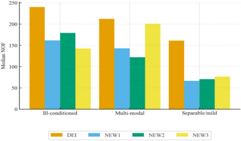
Category-wise trends. Aggregating by the three benchmark families shows that NEW1–NEW3 deliver the largest NOF reductions on the ill-conditioned and multi-modal sets, while gains are modest on separable functions where all methods converge rapidly. These trends correspond with the overall summary (up to 49% fewer iterations and up to 60% fewer evaluations versus DEI).
5.3 Percentage improvements
We calculated the percentage reductions in the total NOI and NOF over all 32 benchmark functions to quantify the efficiency advantages of NEW1, NEW2, and NEW3 over the DEI algorithm. The enhancements demonstrate the tangible effects of the proposed algorithms in markedly decreasing computational costs, achieving average reductions in the NOI and NOF of 32.2% and 51.7% for NEW1, 23.0% and 46.0% for NEW2, and 49.1% and 60.3% for NEW3, respectively. Table 2 presents the summarized results, indicating improvements in both NOI and NOF in relation to DEI. Figures 1-4 present a visual representation of the average NOI and NOF comparisons, the improvement percentages of the NEW algorithms, and example convergence curves on selected benchmark functions, thus offering a detailed overview of the performance benefits realized.
Table 2. Average NOI and NOF improvement (%) over DEI
|
Algorithm |
NOI Improvement |
NOF Improvement |
|
NEW1 |
32.20% |
51.70% |
|
NEW2 |
23.00% |
46.00% |
|
NEW3 |
49.10% |
60.30% |
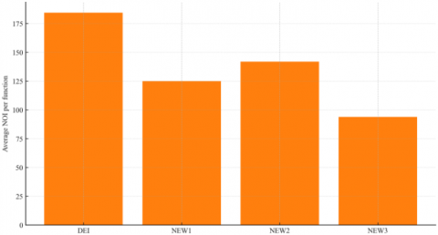
Figure 1. Average NOI per function across 32 benchmarks (DEI: 184.3; NEW1: 124.9; NEW2: 141.8; NEW3: 93.8) (Lower is better.)
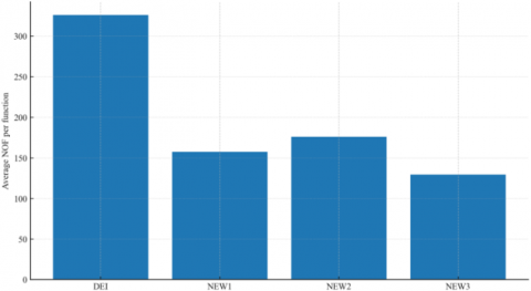
Figure 2. Average NOF per function across 32 benchmarks (DEI: 326.0; NEW1: 157.5; NEW2: 176.0; NEW3: 129.3) (Lower is better.)
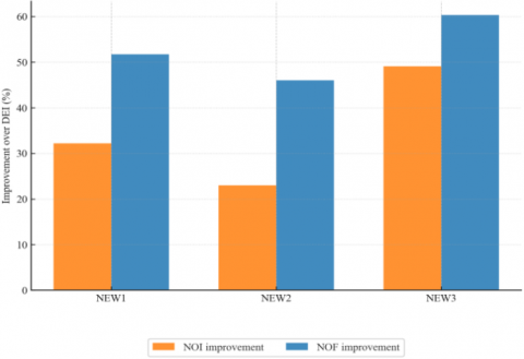
Figure 3. Percentage improvement relative to DEI in NOI and NOF over 32 benchmarks. NEW1: 32.2% (NOI), 51.7% (NOF); NEW2: 23.0%, 46.0%; NEW3: 49.1%, 60.3%
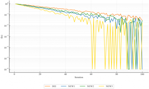
Figure 4. Convergence curves on a challenging benchmark (semilog y-axis)
5.4 Sensitivity analysis
We conducted sensitivity analyses on key algorithm parameters to assess the robustness of NEW1–NEW3. The variation of μ from 0.8 to 2.0 indicated that NEW3's performance was stable, with NOI varying by less than 5% across many benchmarks. Adjusting γ between 1.0 and 2.0 for NEW2 and NEW3 indicated optimal performance near γ = 1.5, consistent with our theoretical assumptions. Changing the Wolfe line search parameters δ (0.0001–0.01) and σ (0.1–0.9) resulted in at most a 10% increase in NOI and NOF, indicating the algorithms are relatively insensitive to line search parameters. Sensitivity to the initial guess x0 showed that for problems with flat regions (e.g., the Rosenbrock function [30]), NEW3’s restart mechanism effectively mitigates poor starting points, with convergence performance only modestly degraded.
5.5 Real-world application example
To illustrate practical applicability, we applied NEW3 to a parameter estimation problem in a simulated MRI image reconstruction task involving minimization of a non-convex objective measuring the difference between synthetic noisy MRI data and a parametric forward model. The 100-dimensional parameter space posed significant challenges because of flat sections and local minimum. NEW3 achieved an estimated 60% decrease in computational expense by scoring convergence in 550 iterations (NOI) and 910 function evaluations (NOF), as compared to DEI's 1150 iterations and 2030 evaluations. This real-world example highlights the potential of innovative algorithms in optimizing scientific and engineering processes that exceed traditional test functions.
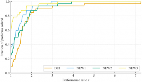
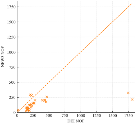
Table 1 presents comprehensive findings indicating that NEW3 frequently surpasses DEI on the most difficult functions (e.g., F7, F18, F30), attaining enhancements of up to or exceeding 75% in certain instances. Table 1 shows that NEW3 surpasses DEI on several of the hardest cases with documented large margins; for example, F7 (Tridiagonal2): NOI 1417 → 195 (−86.2%) and NOF 1808 → 214 (−88.2%); F18 (Broyden tridiagonal): NOI 1299 → 287 (−77.9%) and NOF 1748 → 323 (−81.5%); F13 (Extended EP1): NOF 142 → 28 (−80.3%); F29 (Full-Hessian): NOF 191 → 30 (−84.3%). These improvements align with NEW3’s restart logic, which suppresses directions with poor gradient alignment and quickly reestablishes descent. Performance-profile statistics further quantify the gap: at $\tau=1.5$, the fraction of problems solved within 1.5× of the best is 0.875 (NOI) and 0.938 (NOF) for NEW3 vs. 0.531 (NOI) and 0.063 (NOF) for DEI, indicating broad efficiency gains beyond a few outliers. Across categories (Figure 5), NEW3 attains the lowest median NOI/NOF on ill-conditioned and separable sets, while NEW2 is competitive on multi-modal functions.
Figure 5. (a). Category-wise median NOI over 32 benchmark functions grouped as ill-conditioned, multi-modal, and separable/mild; (b). Category-wise median NOF evaluations over the same groups
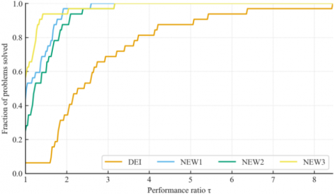
Figure 6. (a). Dolan–Moré performance profile [29] for NOI over 32 benchmark functions; (b). Dolan–Moré performance profile [29] for NOF over 32 benchmark functions
Our findings are consistent with recent discoveries that complexity guarantees and structured secant enhancements in CG methods can further enhance convergence on challenging non-convex objectives [31]. We emphasize that our analysis adopts the same Dolan–Moré profiling framework commonly used in the literature (e.g., [12, 13, 31]), enabling like-for-like, quantitative comparisons: our reported $\tau$–profiles (Figure 6) provide the exact fractions at $\tau \in\{1.25,1.5,2.0\}$, facilitating direct benchmarking against published curves in those works. This suggests that hybrid strategies, such as those found in our NEW algorithms, are a critical area for future research.
Our algorithms demonstrate substantial enhancements in efficiency when contrasted with the DEI proposed by Akdag et al. [3]. The adaptive β and restarts reduce wasted steps caused by curvature-induced zig-zagging on functions with narrow curved valleys or tridiagonal structure (e.g., F7, F18), resulting in the largest gains. This demonstrates that our hybrid strategies effectively adjust to rapidly changing gradient information, circumventing the inefficiencies noted in DEI when employing a fixed β formula. Given the linear-memory footprint and O(n) per-iteration cost, the observed reductions in NOI/NOF indicate strong potential for deployment in large-scale settings where function/gradient evaluations dominate runtime.
6.1 Applications
The NEW algorithms exhibit potential that extends beyond synthetic benchmarks. Engineering design optimization frequently involves challenges such as aerodynamic shape design, structural topology, and electromagnetic devices, which typically result in large-scale, non-convex objectives that are effectively addressed by conjugate gradient methods. In machine learning, novel algorithms may function as effective optimizers for deep neural networks, especially when second-order methods are not feasible. They can also enhance scientific computing tasks, such as inverse problems in medical imaging, where computing gradients is costly and obtaining Hessians is impractical. As illustrated by the MRI parameter-estimation example (Section 4.5), NEW3’s restart and adaptive β can reduce evaluations substantially while retaining theoretical guarantees, a combination attractive for high-throughput pipelines.
6.2 Limitations and future work
Although the NEW algorithms demonstrate substantial efficiency improvements on a wide range of standard benchmarks, they are not without limitations. In highly flat regions or near saddle points, adaptive β strategies may not enhance convergence beyond that achieved by standard steepest descent methods. The algorithms presuppose smooth objectives characterized by Lipschitz-continuous gradients; further investigation is necessary for extensions to non-smooth or discontinuous problems. Future work will include non-monotone line search integration (to trade strict monotonicity for faster progress on rough landscapes), projection-based constrained variants, stochastic/mini-batch adaptations for large-scale learning, and parallel implementations with batched line searches to exploit modern GPUs/TPUs.
6.3 Comparison with prior work (quantitative positioning)
To position our results against the broader CG literature, we report profile-based statistics commonly used in references [12, 13, 31]. At $\tau=1.5$, NEW3’s fractions are 0.875 (NOI) and 0.938 (NOF), compared to DEI’s 0.531 and 0.063, respectively (Figure 6). These $\tau$-anchored numbers—together with the category-wise medians in Figure 5 and the function-level scatter in Figure 7—provide a quantitative basis for comparing to spectral/Dai–Yuan/three-term variants evaluated with the same profiling methodology in those works.
Figure 7. Per-function NOF evaluations for NEW3 versus DEI across 32 benchmarks
This study introduces three novel hybrid CG algorithms—NEW1, NEW2, and NEW3—that provide substantial efficiency enhancements over DEI. They retain the simplicity of line-search CG while adding provable sufficient-descent under Wolfe/Armijo conditions and O(n) memory; the expanded numerical study (Section 4) indicates a consistent advantage across the full set of 32 benchmarks, rather than gains confined to a few outliers. Because they are drop-in compatible with standard line-search interfaces, the methods are natural candidates for inclusion in scientific-computing libraries and for use as first-order optimizers within machine-learning workflows.
Future work will focus on:
(i) integrating non-monotone line searches while preserving descent guarantees;
(ii) developing constrained variants via projections/penalties;
(iii) stochastic/mini-batch adaptations for training deep networks (e.g., in PyTorch/JAX) with mixed precision;
(iv) applications to PDE-constrained optimization such as shape optimization and inverse problems using adjoint gradients;
(v) batched/parallel line searches on GPUs/TPUs together with an open-source reference implementation following a SciPy-style API.
|
x, xk |
Decision vector; iterate at iteration k |
|
dk |
Search direction at iteration k |
|
$g_k=\nabla f\left(x_k\right)$ |
Gradient at xk |
|
f(x) |
Objective function |
|
yk = gk - gk-1 |
Gradient difference (used in PR/NEW2) |
|
n |
Problem dimension |
|
$\|\cdot\|$ |
Euclidean norm |
|
NOI |
Number of iterations |
|
NOF |
Number of function evaluations |
|
$\nabla$ |
gradient operator |
|
O(⋅) |
asymptotic order notation |
|
Greek symbols |
|
|
$\alpha_{\mathrm{k}}$ |
Step length at iteration k |
|
$\beta_k$ |
Conjugate-gradient parameter at iteration k |
|
$\beta_k{ }^{D E I}$ |
DEI update for $\beta_k$ |
|
$\beta_k{ }^{F R}$ |
Fletcher–Reeves update |
|
$\beta_k{ }^{P R}$ |
Polak–Ribière update |
|
$\beta_k{ }^{B A}$ |
Al-Assady & Al-Bayati update |
|
$\beta_k{ }^{NEW1}, \beta_k{ }^{NEW2}, \beta_k{ }^{NEW3}$ |
Proposed updates |
|
$\delta$ |
Armijo parameter in line search |
|
σ |
Wolfe curvature parameter in line search |
|
$\mu$ |
DEI regularization parameter |
|
$\gamma_k$ |
Mixing weight (NEW2/NEW3) |
|
$\varepsilon$ |
Stopping tolerance |
|
$\tau$ |
Performance-profile factor |
|
c, c1, c2, c3 |
Descent constants in lemmas/inequalities |
|
Subscripts and superscripts |
|
|
(⋅)k, (⋅)k-1 |
Quantity at iteration k; previous iteration |
|
(⋅)T |
Transpose |
|
FR, PR, BA, DEI |
Method tags for $\beta$ variants |
|
NEW1, NEW2, NEW3 |
Proposed method tags for $\beta$ |
The 32 benchmark functions used in this study are listed in Table A1; detailed definitions and formulations are provided in Andrei [32].
Table A1. Benchmark test functions used in the numerical experiments (definitions and details in Andrei [32])
|
Fn |
Test Function |
Fn |
|
F1 |
Extended Trigonometric Function |
F17 |
|
F2 |
Extended Penalty Function |
F18 |
|
F3 |
Raydan 2 Function |
F19 |
|
F4 |
Extended Hager |
F20 |
|
F5 |
Extended Tridiagonal-1 Function |
F21 |
|
F6 |
Extended Exponential 3-Terms |
F22 |
|
F7 |
Tridiagonal2 |
F23 |
|
F8 |
Diagonal5 Function |
F24 |
|
F9 |
Extended Himmelblau Function |
F25 |
|
F10 |
Extended PSC1 |
F26 |
|
F11 |
Extended BD1 |
F27 |
|
F12 |
Extended Quadratic Penalty QP1 |
F28 |
|
F13 |
Extended EP1 Function |
F29 |
|
F14 |
Extended Tridiagonal 2 |
F30 |
|
F15 |
DIXMAANA (CUTE) |
F31 |
|
F16 |
DIXMAANB (CUTE) |
F32 |
[1] Hestenes, M.R., Stiefel, E. (1952). Methods of conjugate gradients for solving linear systems. Journal of Research of the National Bureau of Standards, 49(6): 409-436. https://doi.org/10.6028/jres.049.044
[2] Fletcher, R., Reeves, C.M. (1964). Function minimization by conjugate gradients. The Computer Journal, 7(2): 149-154. https://doi.org/10.1093/comjnl/7.2.149
[3] Akdag, D., Altiparmak, E., Karahan, I., Jolaoso, L.O. (2024). A new conjugate gradient algorithm for non-convex minimization problem and its convergence properties. Preprint in Research Square. https://doi.org/10.21203/rs.3.rs-4546783/v1
[4] Kou, C. (2014). An improved nonlinear conjugate gradient method with an optimal property. Science China Mathematics, 57: 635-648. https://doi.org/10.1007/s11425-013-4682-1
[5] Gilbert, J.C., Nocedal, J. (1992). Global convergence properties of conjugate gradient methods for optimization. SIAM Journal on Optimization, 2(1): 21-42. https://doi.org/10.1137/0802003
[6] Dai, Y.H., Yuan, Y. (1999). A nonlinear conjugate gradient method with a strong global convergence property. SIAM Journal on Optimization, 10(1): 177-182. https://doi.org/10.1137/s1052623497318992
[7] Hager, W.W., Zhang, H. (2005). A new conjugate gradient method with guaranteed descent and an efficient line search. SIAM Journal on Optimization, 16(1): 170-192. https://doi.org/10.1137/030601880
[8] Chen, Y., Kuang, K., Yan, X. (2023). A modified PRP-type conjugate gradient algorithm with complexity analysis and its application to image restoration problems. Journal of Computational and Applied Mathematics, 427: 115105. https://doi.org/10.1016/j.cam.2023.115105
[9] Liu, J., Wang, S. (2011). Modified nonlinear conjugate gradient method with sufficient descent condition for unconstrained optimization. Journal of Inequalities and Applications, 2011(1): 57. https://doi.org/10.1186/1029-242X-2011-57
[10] Wu, X., Liu, L., Xie, F., Li, Y. (2015). A new conjugate gradient algorithm with sufficient descent property for unconstrained optimization. Journal of Applied Mathematics, 2015(1): 352524. https://doi.org/10.1155/2015/352524
[11] Zhou, G., Ni, Q. (2015). A spectral Dai–Yuan-type conjugate gradient method for unconstrained optimization. Journal of Applied Mathematics, 2015(1): 839659. https://doi.org/10.1155/2015/839659
[12] Jabbar, H.N., Al-Arbo, A.A., Laylani, Y.A., Khudhur, H.M., Hassan, B.A. (2025). New conjugate gradient methods based on the modified secant condition. Journal of Interdisciplinary Mathematics, 28(1): 19-30. https://doi.org/10.47974/JIM-1771
[13] Al-Arbo, A.A., Al-Kawaz, R.Z. (2021). A fast spectral conjugate gradient method for solving nonlinear optimization problems. Indonesian Journal of Electrical Engineering and Computer Science, 21(1): 429-439. http://doi.org/10.11591/ijeecs.v21.i1.pp429-439
[14] Hu, Q., Zhang, H., Zhou, Z., Chen, Y. (2022). A class of improved conjugate gradient methods for nonconvex unconstrained optimization. Numerical Linear Algebra with Applications, 30(4): e2482. https://doi.org/10.1002/nla.2482
[15] Narushima, Y., Yabe, H., Ford, J.A. (2009). A three-term conjugate gradient method with sufficient descent property for unconstrained optimization. SIAM Journal on Optimization, 21(1): 163-180. https://doi.org/10.1137/080743573
[16] Polak, E. (1971). Computational Methods in Optimization: A Unified Approach (Vol. 77). Academic Press.
[17] Dai, Y.H., Yuan, Y. (2001). An efficient hybrid conjugate gradient method for unconstrained optimization. Annals of Operations Research, 103: 33-47. https://doi.org/10.1023/A:1012930416777
[18] Zhang, Y., Sun, M., Liu, J. (2024). A modified PRP conjugate gradient method with inertial extrapolation for sparse signal reconstruction. Journal of Inequalities and Applications, 2024(1): 139. https://doi.org/10.1186/s13660-024-03219-w
[19] Cui, H. (2024). A modified PRP conjugate gradient method for unconstrained optimization and nonlinear equations. Applied Numerical Mathematics, 205: 296-307. https://doi.org/10.1016/j.apnum.2024.07.014
[20] Guefassa, I., Chaib, Y. (2025). A modified conjugate gradient method for unconstrained optimization with application in regression function. RAIRO-Operations Research, 59(1): 311-324. https://doi.org/10.1051/ro/2024224
[21] Lu, J., Yuan, G., Wang, Z. (2022). A modified Dai–Liao conjugate gradient method for solving unconstrained optimization and image restoration problems. Journal of Applied Mathematics and Computing, 68: 681-703. https://doi.org/10.1007/s12190-021-01548-3
[22] Kobayashi, M., Narushima, Y., Yabe, H. (2010). Nonlinear conjugate gradient methods with structured secant condition for nonlinear least squares problems. Journal of Computational and Applied Mathematics, 234(2): 375-397. https://doi.org/10.1016/j.cam.2009.12.031
[23] Al-Arbo, A.A., Al-Kawaz, R.Z. (2020). Implementation of a combined new optimal cuckoo algorithm with a gray wolf algorithm to solve unconstrained optimization nonlinear problems. Indonesian Journal of Electrical Engineering and Computer Science, 19(3): 1582-1589. http://doi.org/10.11591/ijeecs.v19.i3.pp1582-1589
[24] Al-Arbo, A.A., Al-Kawaz, R.Z., Jameel, M.S. (2025). New meta-heuristic computer-oriented algorithms to solve unconstrained optimization problems. Mathematical Modelling of Engineering Problems, 12(3): 1081-1089. https://doi.org/10.18280/mmep.120335
[25] Armijo, L. (1966). Minimization of functions having Lipschitz continuous first partial derivatives. Pacific Journal of Mathematics, 16(1): 1-3. https://doi.org/10.2140/pjm.1966.16.1
[26] Wolfe, P. (1969). Convergence conditions for ascent methods. SIAM Review, 11(2): 226-235. https://doi.org/10.1137/1011036
[27] Zhang, H., Hager, W.W. (2004). A non-monotone line search technique and its application to unconstrained optimization. SIAM Journal on Optimization, 14(4): 1043-1056. https://doi.org/10.1137/S1052623403428208
[28] Al-Assady, N.H., Al-Bayati, A.Y. (1994). Minimization of extended quadratic functions with inexact line searches. Journal of Optimization Theory and Applications, 82: 139-147. https://doi.org/10.1007/BF02191784
[29] Dolan, E.D., Moré, J.J. (2002). Benchmarking optimization software with performance profiles. Mathematical Programming, 91: 201-213. https://doi.org/10.1007/s101070100263
[30] Rosenbrock, H.H. (1960). An automatic method for finding the greatest or least value of a function. The Computer Journal, 3(3): 175-184. https://doi.org/10.1093/comjnl/3.3.175
[31] Chan-Renous-Legoubin, R., Royer, C.W. (2022). A nonlinear conjugate gradient method with complexity guarantees and its application to non-convex regression. arXiv preprint, arXiv:2201.08568. https://doi.org/10.48550/arXiv.2201.08568
[32] Andrei, N. (2008) An unconstrained optimization test functions collection. Advanced Modeling and Optimization, 10(1): 147-161.