Siva Tejaswi Jonna![]() | Karthika Natarajan*
| Karthika Natarajan*![]()
© 2025 The authors. This article is published by IIETA and is licensed under the CC BY 4.0 license (http://creativecommons.org/licenses/by/4.0/).
OPEN ACCESS
Epileptic seizures affect over 50 million people globally, posing significant diagnostic and safety challenges due to their sudden and unpredictable nature. This study proposes a hybrid deep learning model that combining Discrete Wavelet Transform (DWT), Convolutional Neural Networks (CNN), and Long Short-Term Memory (LSTM) networks to predict seizures using EEG signals. SHapley Additive exPlanations (SHAP) are integrated to provide interpretability at both global and local levels. The model is trained and evaluated on the Bonn EEG dataset and achieving 98% accuracy, 98% recall, and 98.7% precision. SMOTE is applied to address class imbalance, which improving recall and F1-score. Min-Max normalization preserves amplitude dynamics essential for EEG analysis. While the Bonn dataset provides clean, balanced signals suitable for benchmarking, further validation on real-world datasets is recommended to enhance clinical applicability. The proposed framework demonstrates strong potential for real-time seizure prediction with interpretable insights to support personalized epilepsy care.
electroencephalography, epileptic seizures, long short-term memory (LSTM), SHapley Additive exPlanations, wavelet convolutional neural network (CNN)
Epilepsy, a neurological disorder affecting approximately 50 million people worldwide, is characterized by recurrent, unprovoked seizures resulting from abnormal electrical activity in the brain [1]. Early and accurate seizure prediction is crucial, especially for patients with drug-resistant epilepsy, to enhance safety and quality of life. Electroencephalogram (EEG) signals offer a non-invasive, real-time method for monitoring brain activity and detecting epileptic events. However, manual interpretation of EEG is time-intensive and subject to inter-observer variability, prompting the adoption of artificial intelligence (AI) techniques for automated seizure prediction [2, 3].
Machine learning (ML) and deep learning (DL) approaches have demonstrated potential in analyzing complex EEG patterns, yet they often struggle with capturing intricate spatiotemporal features and providing transparent decision-making processes [4, 5]. To overcome these challenges, recent works have proposed hybrid architectures—combining convolutional neural networks (CNNs) for spatial feature extraction and long short-term memory (LSTM) networks for temporal modeling [6, 7]. Although effective, these models typically function as "black boxes," limiting clinical trust due to their lack of interpretability.
To improve transparency, explainable AI (XAI) methods such as SHapley Additive exPlanations (SHAP) have been introduced to interpret model outputs. Nonetheless, most current applications remain at a preliminary stage and have yet to demonstrate consistent clinical relevance [8, 9]. Complementing these developments, recent studies underscore the broader role of ML and DL in EEG-based neurological disorder analysis, enhancing predictive power and interpretability [10].
Despite these advances, many studies emphasize accuracy while relying on idealized datasets that lack real-world clinical complexity. Moreover, they often neglect computational efficiency and clinical interpretability. Addressing these gaps, this study proposes a novel Wavelet CNN-LSTM model with SHAP-based interpretability for early epileptic seizure prediction. Key contributions include: the use of Discrete Wavelet Transform (DWT) for noise-resilient, time-frequency feature extraction; a CNN-LSTM hybrid for robust spatial-temporal learning; and SHAP integration to facilitate transparent, clinically meaningful model interpretation.
Epilepsy affects nearly 50 million people worldwide, with seizures that are often unpredictable and disruptive. To improve detection and prediction, various ML and DL techniques have been applied to EEG signals. Vieira et al. [11] proposed an explainable AI model using simple classifiers and selected EEG features, achieving over 95% accuracy, but lacking temporal modeling due to the absence of deep learning. Chowdhury and Chowdhury [12] used a quantum machine learning model with MRI and Layer-wise Relevance Propagation (LRP), showing strong performance but limited real-time usability due to high computational cost. Our proposed CNN-LSTM model with SHAP improves both accuracy and interpretability using EEG, optimized for real-time clinical application.
Zhang et al. [13] introduced a DNN with adversarial training and attention mechanisms to improve generalization, though it increased model complexity. Our method achieves similar robustness without adversarial overhead by combining wavelet-based spatial and LSTM-based temporal features. Lo Giudice et al. [14] developed a CNN to differentiate epileptic and psychogenic seizures, but limited data and lack of temporal analysis reduced generalizability. We address this through LSTM layers and larger dataset validation. Al-Hussaini and Mitchell [15] presented SeizFt using wearable EEG, data augmentation, and CatBoost, improving sensitivity but struggling with diverse seizure types. Our model enhances robustness by integrating DWT, CNN, and LSTM for more comprehensive and interpretable predictions.
Although considerable progress has been made in epileptic seizure detection, key challenges remain. Many existing models inadequately capture both the frequency and temporal features of EEG signals, resulting in reduced accuracy and poor generalizability across patient datasets [11, 16]. Additionally, high computational complexity and limited scalability hinder their integration into real-time clinical applications [12]. A further limitation is the lack of interpretability in deep learning models, which often operate as black boxes, thereby limiting trust in clinical decision-making processes [17, 18].
To address these limitations, we propose a hybrid deep learning framework that combines DWT for multi-resolution frequency feature extraction, CNN for learning spatial patterns, and LSTM networks for capturing temporal dependencies. Furthermore, SHAP is employed to provide both global and local interpretability of model predictions [6, 18].
This integrated approach leverages the strengths of DWT, CNN, and LSTM to improve the detection of seizure-related EEG patterns. The incorporation of SHAP enhances transparency, providing insights into the contribution of individual features. As a result, the model achieves better prediction accuracy, supports real-time implementation, and fosters clinical trust, offering a comprehensive solution for early seizure prediction and intervention planning [19, 20].
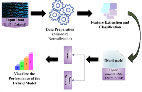
To capture spatial, frequency, and temporal EEG dynamics, a hybrid model was developed using DWT, CNN, LSTM networks, and SHAP. DWT decomposes EEG signals into sub-bands for frequency-domain features [21], which are processed by CNN layers for spatial learning and LSTM layers for temporal pattern recognition [22]. A dense layer handles binary classification, using ReLU activation, max-pooling, and residual connections for deeper learning [23]. SHAP provides global and local interpretability, revealing feature contributions to predictions (Figure 1).
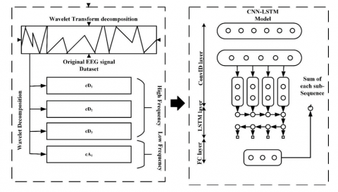
While the model performed well on the clean Bonn EEG dataset, its limited complexity restricts generalizability [24]. The early plateau in validation loss suggests overfitting. Future work includes testing on more diverse datasets like CHB-MIT [25] and UBMC [17], and applying regularization (e.g., dropout, early stopping). The workflow (Figure 1) includes EEG acquisition, normalization, model training, evaluation, and SHAP analysis. As illustrated in Figure 2, the architecture starts with wavelet decomposition (cA1, cD1–cD3), followed by CNN-LSTM feature extraction, classification, and interpretability. This integrated design boosts predictive accuracy, transparency, and clinical relevance for early seizure prediction.
Figure 1. Proposed methodology for Hybrid Wavelet CNN-LSTM-SHAP
Figure 2. Architecture of the proposed Hybrid Wavelet CNN-LSTM model
4.1 Data collection
The EEG dataset used in this study consists of 500 recordings, grouped into five subsets of 100 files each, where each file captures 23.6 seconds of brain activity, represented by 4,097 time-series data points [24]. These recordings were segmented into 23 segments per file, each with 178 data points corresponding to one-second EEG intervals. This results in a matrix of 11,500 rows (segments) and 178 columns (features), with the 179th column representing the class label $y \in \{1.2 .3 .4 .5\}$. The class labels denote specific brain states: Class 1 (epileptic seizure), Class 2 (tumor region), Class 3 (healthy region in tumor patients), Class 4 (eyes closed), and Class 5 (eyes open). Classes 2 to 5 represent non-epileptic activity, and many studies treat the dataset as a binary classification task: seizure (Class 1) vs. non-seizure (Classes 2–5).
The dataset was split randomly into training (70–80%), validation (10–15%), and testing (10–15%) sets. This stratification ensured fair evaluation of model generalization. The training set was used for model learning, the validation set for tuning hyperparameters, and the testing set for final performance assessment on unseen data.
4.2 Data pre-processing and balancing
Data pre-processing enhances learning efficiency by modifying input features to a standardized scale. In this study, Min-Max normalization was applied to rescale EEG signals to a range of 0 to 1. This approach reduces computational complexity, accelerates convergence, and preserves relative amplitude variations critical for detecting seizure-related anomalies. Unlike Z-score normalization, which may obscure these patterns, Min-Max scaling ensures that all features contribute proportionally to the model [5, 11]. The normalization is defined by:
$\begin{aligned} u_0=\left(\left(y_0-y_{0_{\text {min}}}\right)\right. & (\max -\min)) /\left(\left(y_{0_{\text {max}}}-y_{0_{\text {min}}}\right)+\min \right)\end{aligned}$ (1)
where, u₀ is the normalized value, y₀ is the original input, and (min, max) represent the target range.
Although the CHB-MIT dataset is commonly used for real-world clinical evaluations, we employed the Bonn EEG dataset due to its clean, balanced structure and high signal quality, which make it suitable for benchmarking deep learning models. To address class imbalance—especially the underrepresentation of seizure cases (Class 1)—the Synthetic Minority Over-sampling Technique (SMOTE) was applied. As shown in Table 1 (before SMOTE and after SMOTE), this technique balanced the class distribution, enhancing recall and F1-score for seizure detection while maintaining high precision across all classes. This data preparation pipeline supports the robustness and generalizability of the proposed Wavelet CNN-LSTM-SHAP model and establishes a foundation for future testing on more complex datasets like CHB-MIT [26, 27].
SMOTE (Synthetic Minority Over-sampling Technique) is a popular technique for balancing imbalanced data by creating synthetic samples for minority classes. In the pre-processing step, SMOTE selects a sample from a minority class and works to find its k-nearest neighbours. For each selected model, an artificial model is generated by interpolation between the model and its neighbours. For each selected model, an artificial model is generated by interpolation between the model and its neighbours. The equation for the artificial sample xn is given by:
$x_n=x_i+\lambda \times\left(x_{n n}-x_i\right)$
where, $x_i$ is a subclass sample, $x_n$ is one of its nearest neighbours k, and λ is a random number ranging from 0 to 1. This process is repeated until equilibrium is reached, contributing to machine learning modelling variety is effective. More classes are adequately represented during training.
The Bonn EEG dataset was selected for its clean signals, balanced class labels, and controlled conditions—ideal for validating deep learning models. In contrast, the CHB-MIT dataset offers more clinical realism but includes high noise, patient variability, and temporal imbalance, requiring extensive preprocessing and personalized models [24, 25]. Thus, the proposed method establishes a strong baseline for future application to more complex EEG datasets.
Table 1. Comparison of model performance before and after SMOTE balancing
|
Metric |
Before SMOTE |
After SMOTE |
|
Accuracy |
96.3% |
98.0% |
|
Precision |
94.5% |
98.5% |
|
Recall |
91.2% |
98.0% |
|
F1-Score |
92.8% |
98.0% |
|
Minority Class Sensitivity (Class 1) |
88.4% |
97.8% |
4.3 Feature extraction and classification using Hybrid Wavelet CNN-LSTM-SHAP
The DWT is a mathematical technique that decomposes signals into time-frequency components, offering advantages over traditional Fourier transforms by capturing both frequency and location information. DWT is particularly effective for multi-scale analysis of complex sequences, making it suitable for EEG signal processing.
Using wavelet decomposition, the EEG signal is split into two parts: approximation coefficients (low-frequency components) and detail coefficients (high-frequency components). The approximation captures the primary structure of the signal, while the detail contains transient or noisy information. This allows for effective noise reduction by isolating and discarding high-frequency fluctuations, improving feature quality for downstream analysis using the hybrid CNN-LSTM-SHAP model.
To compute a set of wavelets $\psi^{\prime}{ }_{j, k}(t)$ and binary scalefunctions $\varphi^{\prime}{ }_{j, k}(t)$ for a given wavelet's mother function $\psi^{\prime}(t)$ and its associated scaling function $\phi^{\prime}(t)$, use the Eqs. (2) and (3):
$\psi_{j, k}^{\prime}(t)=2^{\frac{j}{2}} \psi^{\prime}\left(2^j t-k\right)$ (2)
$\varphi_{j, k}^{\prime}(t)=2^{\frac{j}{2}} \varphi^{\prime}\left(2^j t-k\right)$ (3)
in where $t, j$, and $k$ signify the time indices, scaling variables, and translating variables. The initial sequences $o s^{\prime}(t)$ may be represented as shown in Eq. (4):
$\begin{gathered}o s^{\prime}(t)=\sum_{k=1}^n c_{j, k}^{\prime} \varphi_{j, k}^{\prime}(t)+ \sum_{j=1}^J \sum_{k=1}^n d_{j, k}^{\prime} \psi_{j, k}^{\prime}(t)\end{gathered}$ (4)
In this equation, $c^{\prime}{ }_{j, k}$ represents the approximate coefficient for scale $j$ and location $k, d^{\prime}{ }_{j, k}$ represents the comprehensive coefficients at scale $j$ and locations $k, n$ is the initial sequence size, and $J$ is the breakdown levels. According to the rapid DWT, the approximation sequence and the complete sequence within a specific WD level may be derived using numerous low and high-pass filters.
The proposed Hybrid Wavelet CNN-LSTM model (Figure 2) combines DWT, CNN, and LSTM to extract spatial, spectral, and temporal features from EEG signals for early seizure prediction. DWT, using the Daubechies 4 (db4) wavelet, is selected for its effective time-frequency localization and proven utility in biomedical signal analysis [21, 22]. The EEG signals are decomposed into three levels, yielding one approximation (cA3) and three detail coefficients (cD3, cD2, cD1) that preserve essential signal characteristics linked to seizure onset. These coefficients are then passed into a CNN with two convolutional layers (32 and 64 filters, 3×3 kernels), followed by ReLU activations, batch normalization, dropout (rate = 0.25), and 2×2 max-pooling. Residual connections are added to retain low-level spatial features and improve training stability [23].
The CNN output is flattened and passed to a stacked LSTM network for modeling temporal dependencies. The first LSTM layer (128 units, return_sequences=True) and the second (64 units) capture sequential patterns in the EEG. A final dense layer with a sigmoid activation performs binary classification (seizure vs. non-seizure). The model is trained using the Adam optimizer (learning rate = 0.001), binary cross-entropy loss, batch size of 64, and 100 epochs. Performance is measured using accuracy, precision, recall, and F1-score. Compared to Short-Time Fourier Transform (STFT), DWT offers adaptive resolution and improved localization of transient seizure activity [11]. For interpretability, SHAP quantifies each feature’s influence on predictions, providing both global and local insights to support clinical transparency and trust [18].
4.3.1 Convolutional layer
The process of convolution is characterized as a particular linear approach for extracting local patterns in temporal domains and identifying local correlations in the input sequence. Eqs. (5) and (6) define the fundamental sequence input S as well as the filter sequences FS. Vectors are shown in bold according to the standard.
$S^{\prime}=\left[s_1^{\prime}, s_2^{\prime}, s_3^{\prime}, \ldots s_L^{\prime}\right]$ (5)
$F S^{\prime}=\left[\omega_1^{\prime}, \omega_2^{\prime}, \omega_3^{\prime}, \ldots \omega_K^{\prime}\right]$ (6)
In this example, $s_i^{\prime} \in R$ represents a sequence of data points arranged by time, while $\omega_j^{\prime} \in R^{\prime(m \times 1)}$ represents the filtering vectors. $L$ the lengths of initial sequence inputs $S$, whereas $K$ is the total amount of filtering in the convolutional layers. Eq. (7) defines the convolution process as a product of a filter vector $\omega_j^{\prime}$ and a combination of vectors $s_{i: i+m-1}^{\prime}$.
$s_{i: i+m-1}^{\prime}=s_i^{\prime} \oplus s_{i+1}^{\prime} \oplus s_{i+2}^{\prime} \oplus s_{i+m-1}^{\prime}$ (7)
The combination operator is $\bigoplus$, and $s_{i: i+m-1}^{\prime}$ represents a window of $m$ continual timing steps beginning with the $i$-th step. Furthermore, the term "bias" $b \in R$ would be addressed throughout the convolution procedure. Therefore, the last calculating equation is expressed in Eq. (8).
$c_i^{\prime}=f\left(\omega_j^{\prime T} s_{i: i+m-1}^{\prime}+b\right)$ (8)
$\omega_j^{\prime T}$ is the transposed of the filtering matrix $\omega_j^{\prime}$, and $f$ is a nonlinear activation function. Furthermore, indices $i$ specifies the $i$-th timing steps, while index $j$ represents the $j$-th filters.
The incorporation of activated functions aims to improve the models' ability to acquire big and complex functions, hence increasing prediction performance. Using an effective activation function may not just accelerate convergence but additionally improve model complexity. Rectified Linear Units are utilized in simulations because they exceed other types of activation mechanisms.
An activation function called Rectified Linear Unit (ReLU) comes after each convolutional layer. Data can go from the first to final layers to residual learning blocks. Moreover, these blocks are utilized to optimize CNN loss by concatenating the retrieved features from several convolutional layers. One of the most important parts of the residual learning block is depth concatenation [23]. The feature map's depth is increased by using depth concatenation. A convolutional layer, a batch normalization layer, and a ReLU function comprise each convolutional block.
4.3.2 Pooling layer
The preceding sample only shows the specific convolution operations technique among a single filter and the input sequences. A single filter can produce one features map. Numerous filters are used in the convolutional layer to effectively extract the main properties of input data. The convolutional layer has K filters having a windows size of m, as previously assumed. In Eqs. (6) and (8), every vector $\omega_j^{\prime}$ denotes a filter, and the single value $c_i^{\prime}$ indicates the window activations.
The convolutional operation across the full sequence input is carried out by moving filtering windows from the first to the last timing step. As a result, the features map related to that filter may be represented using a vector, as shown in the Eq. (9).
$F_j^{\prime}=\left[c_1^{\prime}, c_2^{\prime}, c_3^{\prime}, \ldots c_{L-m+1}^{\prime}\right]$ (9)
The items in $F_j^{\prime}$ represent multi-windows as $\left\{s_{1: m}^{\prime}, s_{2: m}^{\prime}, \ldots s_{1-m+1: L}^{\prime}\right\}$. Index $j$ represents the $j$-th filter.
Pooling is equivalent to sub sampling since it subsects the result of a convolutional layers depending on a certain pooling size $p$. This indicates that the pooling layers may efficiently condense the length of the features map, thereby reducing the amount of model parameters. The model's max-pooling method yields the compressed vector of features $F_j^{\prime}-$compress, as shown below. Also, the max function requires a max functional over the p successive elements in the features map $F_j^{\prime}$ in Eq. (10).
$F_j^{\prime}-$ compress $=\left[h_1^{\prime}, h_2^{\prime}, h_3^{\prime}, \ldots h_{\frac{L-m}{p}+1}^{\prime}\right]$ (10)
where, $h_j^{\prime}=\max \left(c_{(j-1) p}^{\prime}, c_{(j-1) p+1}^{\prime}, \ldots, c_{j p-1}^{\prime}\right)$.
The CNN-based extractors of features can produce accurate and relevant data than the original sequencing input. Furthermore, compressing the duration of the sequences of inputs improves the capacity of future LSTM models to collect temporal information.
The CNN output, which contains spatial information gleaned from EEG, is fed into the LSTM layers. This allows the model to analyse long-term trends in EEG data and produce precise predictions by capturing temporal dependencies that are essential for seizure prediction.
The conventional neural networks structures are differentiated by fully connected among neighbouring levels, that may translate the present input into target vectors. Yet, RNN can maps the target vectors utilizing the complete past of prior inputs. RNN outperforms traditional neural networks for simulating dynamics in sequential data. Overall, RNN joins units from guided cycles and remembers previous inputs via internal states. RNN results at time intervals t−1 may have an influence on RNN results at time steps t. This permits RNN to form temporal links between the current patterns and the previous ones [22].
The consecutive vectors $X=[x(0), x(1), x(2)]$ are fed into RNN one by one based on the timing step. This is distinct from a standard feed-forward networks, where all sequencing vectors are supplied into the framework at the same time. The applicable formula can be stated as follows in Eq. (11).
$S^{\prime}(t)=\sigma\left(U \cdot x^{\prime}(t)+W \cdot S^{\prime}(t-1)+b\right)$ (11)
$y^{\prime}(t)=\sigma\left(V \cdot s^{\prime}(t)+c\right)$ (12)
The equation shows that $x^{\prime}(t)$ is the initial variables at the t time steps. $W, U$ and $V$ are weight matrices. $b$ and $c$ are biased vectors, $\sigma$ is a function of activation, and $y^{\prime}(t)$ is the result that is anticipated at a $t$ times in Eq. (12).
While RNN excels in simulating dynamics in sequential data, it could be impacted by the gradient vanishing and inflating issue during backpropagation-based training of models when analysing longer sequences. Consider the inherent shortcomings of standard RNN, its enhanced form, termed LSTM, is used in this study, as described in the following section.
The LSTM network is a kind of RNN that integrates representations learning and model construction without needing additional domain expertise. The improved LSTM architecture helps to eliminate gradient disappearance and explosive issues in standard RNN. This demonstrates that LSTM is more successful in collecting long-term connections and simulating nonlinear structures when dealing with sequential data that is longer in period.
LSTM is specifically developed to avoid the issue of gradient vanishing, allowing the connection among vectors in the shorter and longer terms to be retained. In an LSTM cell, $h^{\prime}(t)$ represents a short-term state, whereas $c^{\prime}(t)$ represents a longer-term state. The major feature of LSTM is its ability understand which should be preserved in the long term., which should be rejected, and which should be read. When the $c^{\prime}(t-1)$ point reaches the cell, it first travels via a forget gates to remove memory; next the new memory are inserted into it through an input gate; at last, a novel outcome $y^{\prime}(t)$ is produced and processed by the resultant gate. The mechanism of where new recollections originates those gates operate is demonstrated below.
(1) Forget Gate
This section describes that LSTM determines what kind of data is allowed into the memories cell. After passing through the sigmoid function, $h^{\prime}(t-1)$ and $x^{\prime}(t)$ create a value $f^{\prime}(t)$ ranging from 0 to 1. A value of 1 indicates that $h^{\prime}(t-1)$ would be completely incorporated in the cells state $c^{\prime}(t-1)$. If the current value is 0 , cell state $c^{\prime}(t-1)$ will forsake $h^{\prime}(t-1)$. The formula for this procedure is presented below in Eq. (13):
$f^{\prime}(t)=\sigma\left(W_f^{\prime} \cdot\left[h^{\prime}(t-1), x^{\prime}(t)\right]+b_f^{\prime}\right)$ (13)
in which $W_f^{\prime}$: weighted matrix, $b_f^{\prime}$: bias vectors, and $\sigma$ is the activation factor.
(2) Store Gate
This section explains that LSTM determines which types of data can be kept within the cell's state. The sigmoid function is used to transform $h^{0 \prime}(t-1)$ into a value ranging from 0 to 1. The $\tanh$ function is then used to transform $h^{0 \prime}(t-1)$ into an alternative potential value, $g^{0^{\prime}}(t)$. Finally, the two outputs described above are combined to update the prior state, as shown in Eqs. (14) and (15).
$i^{0 \prime}(t)=\sigma\left(w_i^{\prime} \cdot\left[h^{0 \prime}(t-1), x^{\prime}(t)\right]+b_i^{\prime}\right)$ (14)
$g^{0 \prime}(t)=\tanh \left(w_g^{\prime} \cdot\left[h^{0 \prime}(t-1), x^{\prime}(t)\right]+b_g^{\prime}\right)$ (15)
The prior cell state $c^{0 \prime}(t-1)$ decides which information to discard and store before creating the next cell state $c^{0 \prime}(t)$. This procedure may be expressed as follows in the Eq. (16).
$c^{0 \prime}(t)=f^{\prime}(t) \cdot c^{0 \prime}(t-1)+i^{0 \prime}(t) \cdot g^{0 \prime}(t)$ (16)
(3) Output Gate
The LSTM outputs is dependent on the modified cell state $c^{\prime}(t)$. Initially, use the sigmoid functions to create a value $o^{\prime}(t)$ to regulate output. The cell state $h^{\prime}(t)$ is generated by using $\tanh$ and the outcome of the sigmoid function $o^{\prime}(t)$. After the aforementioned process, produce $y^{\prime}(t)$, as illustrated in the two Eqs. (17) and (18).
$o^{\prime}(t)=\sigma\left(w_o^{\prime} .\left[h^{\prime}(t-1), x^{\prime}(t)\right]+b_o^{\prime}\right)$ (17)
$y^{\prime}(t)=h^{\prime}(t)=o^{\prime}(t) * \tanh \left(C^{\prime}(t)\right)$ (18)
The EEG analysis pipeline integrates signal processing and deep learning to enable effective seizure prediction. It begins with collecting raw EEG data, which is decomposed using Wavelet Transform into four frequency components: cD3 (high-frequency), cD2 (mid-frequency), cD1 (low-frequency), and cA1 (approximation). These components are then passed to a CNN-LSTM model, where the convolutional layer extracts spatial features and LSTM layers handle temporal patterns. The model processes these components sequentially, and its output is derived by summing the learned sub-sequences.
This architecture first applies Wavelet Transform to separate the EEG signal into discrete detail (cD) and approximation (cA) coefficients. These are input into the CNN-LSTM model, where CNN layers extract local patterns and LSTM layers capture sequential dependencies while filtering irrelevant information. The extracted features are combined and aggregated to form a comprehensive representation of the EEG signal. This hybrid approach effectively leverages both wavelet decomposition and deep learning for EEG analysis, making it well-suited for tasks like epileptic seizure prediction.
4.4 Explainable AI (XAI)
Interpreting ML model predictions is essential for clinical trust and decision-making. While simpler models offer transparency, they often lack the accuracy of deep learning approaches. To balance this trade-off, SHAP provide a unified method to interpret outputs across different ML models, including complex neural networks [18].
SHAP extends game theory’s Shapley values to quantify each feature's contribution to a prediction. It supports global interpretability by ranking overall feature importance and local interpretability by explaining individual outcomes. Unlike traditional techniques, SHAP delivers case-specific insights, improving transparency and trust. It is also model-agnostic, supporting both linear and non-linear architectures.
Integrated into the proposed Wavelet CNN-LSTM model, SHAP highlights the most influential EEG features in seizure prediction. It supports various explanation modes:
This study integrates SHAP into the Wavelet CNN-LSTM model to provide both global and local interpretability, enabling transparent identification of the most influential EEG features in seizure prediction through text, local, representative, and visual explanation modes.
The proposed hybrid model outperformed previous techniques in the early prediction of epileptic seizures, displaying robust performance across a wide range of patient datasets. Furthermore, SHAP analysis gave a significant understanding of the contributing components of seizure prediction, improving the ability to interpret and comprehension of the underlying processes.
5.1 Input data visualization
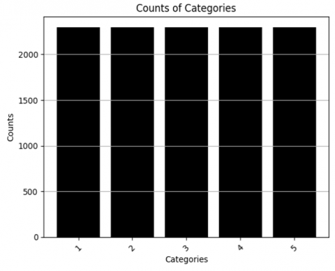
To address class imbalance and better reflect real-world seizure distribution, SMOTE was applied. As shown in Figure 3, the seizure class (Class 1) was initially underrepresented. Post-SMOTE, class distribution was balanced, significantly improving recall and F1-score without reducing precision. EEG features were normalized using Min-Max scaling to map values to [0, 1], preserving amplitude structure critical for detecting seizure patterns. This method outperforms Z-score normalization, which may suppress key signal characteristics [5, 11]. Figure 4 presents a bar graph depicting the number of categories, with the y-axis marked 'Counts' (0–2000) and the x-axis labelled with category numbers from 1 to 5. Each of the five equally spaced bars reaches the 2000-count marker, indicating that every category has an equal count of 2000.
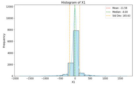
The frequency distribution of EEG signal values (X1) is shown in Figure 4. The frequency is represented by the y-axis, which varies from 0 to 12000, while the X1 is represented by the x-axis, which runs from -2000 to 1500. On the X1 axis, the bars are concentrated in the region between -500 and 0. Measures of statistics are shown. A dashed line at -11.58 represents the mean, a dashed line at -8.00 represents the median, and a dashed line at 165.63 represents the standard deviation.
Figure 3. Data visualization distribution
Figure 4. Histogram of EEG signals [24]
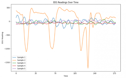
Figure 5. EEG readings over time [24]
Figure 5 displays five EEG samples. Samples 1 and 4 show stable readings, while Samples 2 and 3 have minor, similar fluctuations. Sample 5 shows sharp peaks and troughs. The x-axis (0–175) represents time, and the y-axis (-1500 to 500) indicates EEG amplitude. The graph highlights EEG activity changes over time.
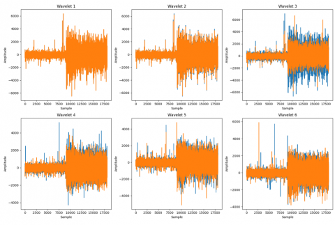
Figure 6 shows the six-level wavelet decomposition of EEG signals illustrating amplitude variations across samples for seizure (orange) and non-seizure (blue) segments.
Figure 6. Wavelet features of different channels
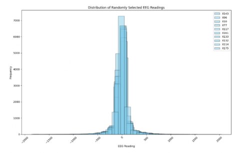
Figure 7. Distribution of randomly selected EEG readings [24]
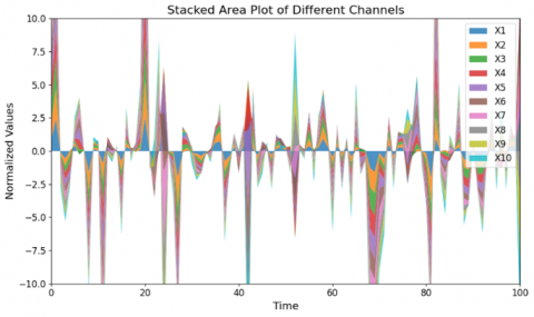
Figure 8. Different channels stacked area plot [24]
Figure 7 presents a histogram of EEG values. The x-axis (−2000 to 2000) shows EEG readings, and the y-axis (0 to 7000) indicates frequency. Most bars cluster around zero. The legend includes randomly selected EEG groups labeled x55, x86, x22, x34, x46, x139, x73, x68, x174, and x175, illustrating the data distribution.
Figure 8 visualizes data from channels X1 to X10, each shown in a different color. The x-axis (0–100) represents time, and the y-axis (−10.0 to 10.0) shows normalized values. Stacked regions illustrate variations across channels over time, with sharp peaks and troughs indicating differences in normalized values.
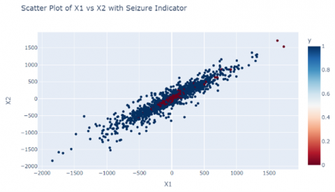
Figure 9 shows a scatter plot of seizure prediction, with data points representing distinct channels. Channels: The scatter plot has two sorts of data points: '0' and '1'. X1 ranges from -2000 to 1500. X2 ranges from -2000 to 1500. Distribution points are more prevalent and spread out while clustering at the core.
Figure 9. Scatter plot of different channels [24]
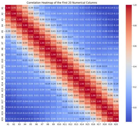
Figure 10. Correlation heat map [24]
Figure 10 shows correlations among variables X1 to X20. Values near 1 indicate strong positive, and near -1 indicate negative correlation. Color intensity reflects strength, with a diagonal of 1s showing self-correlation. The heatmap aids in pattern recognition and data analysis.
5.2 Prediction output
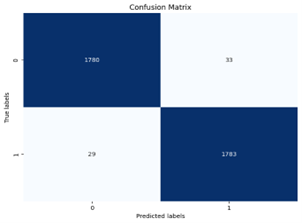
Figure 11 illustrates the performance of the seizure prediction model using a confusion matrix. The x-axis shows predicted labels (0: no seizure, 1: seizure), and the y-axis shows actual labels. The matrix includes: 1788 True Negatives, 24 False Positives, 15 False Negatives, and 1798 True Positives. It is used to evaluate accuracy, recall, precision, and F1-score.
Figure 11. Confusion matrix of seizure prediction
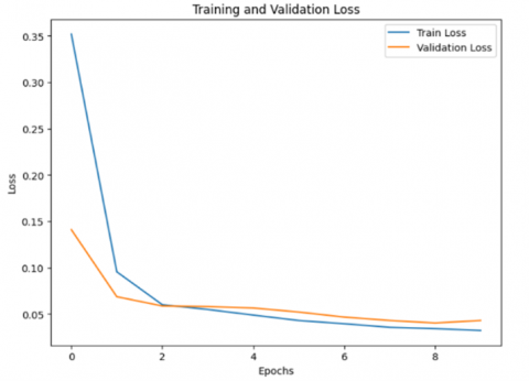
Figure 12. Training and validation loss
Figure 12 shows the training and validation loss over epochs, indicating model performance during training. Loss measures the gap between predicted and actual values. Training loss starts high and quickly drops near zero. Validation loss starts lower, declines gradually, and stabilizes above zero. The graph helps monitor convergence and overfitting.
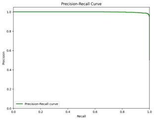
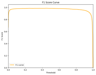
Figures 13 and 14 illustrate key evaluation metrics for binary classification. In Figure 13, the Precision-Recall Curve plots Precision (y-axis) against Recall (x-axis), showing high precision with low recall initially, and performance indicated by the area under the curve. Figure 14 presents the F1 Score Curve, starting at 0 and rising sharply to a peak of 1.0, then gradually declining as the threshold nears 1.0.
Figure 13. Precision-recall curve [26, 27]
Figure 14. F1 score curve [26, 27]
Table 2. Performance comparison
|
Metrics |
Precision |
Recall |
Accuracy |
F1-Score |
|
RIPPER-SVM-NN [26] |
0.85 |
0.85 |
0.857 |
0.85 |
|
ZC in WT-SVM [27] |
0.96 |
0.90 |
0.94 |
0.92 |
|
CNN-LSTM |
0.97 |
0.94 |
0.96 |
0.95 |
|
Hybrid Wavelet CNN-LSTM-SHAP |
0.987 |
0. 98 |
0.98 |
0.98 |
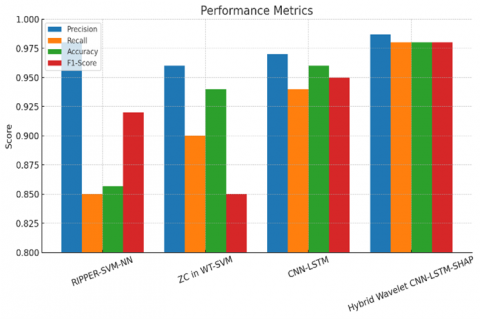
Table 2 presents precision, recall, accuracy, and F1-score for various seizure prediction models. While RIPPER-SVM-NN shows reasonable accuracy, the Hybrid Wavelet CNN-LSTM-SHAP model achieves superior performance, particularly in early seizure prediction.
The performance metrics of three different machine learning algorithms are shown in Figure 15. Maximum precision is attained by RIPPER-SVM-NN [16], maximum recall is attained by ZC in WT-SVM [11], and higher accuracy is demonstrated by Hybrid Wavelet CNN-LSTM-SHAP. Furthermore, the F1-scores for ZC in WT-SVM and RIPPER-SVM-NN are 85% and 92%, whereas CNN-LSTM and Hybrid Wavelet CNN-LSTM-SHAP exceeds 95%, providing important information on how well the models perform under various assessment criteria.
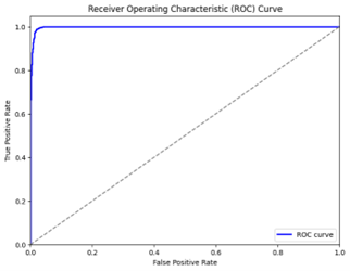
The model's performance is shown by the ROC curve in Figure 16, which has an AUC-ROC value o demonstrates the model's capacity to discriminate between true positive and false positive rates. The model's efficacy is shown by the curve, which is positioned considerably above the diagonal line. Higher AUC values correspond to better classification performance.
Figure 15. Comparison of performance metrics [11, 16, 26, 27]
Figure 16. ROC curve [24-27]
Table 3. Performance of computational time
|
Methods |
Time |
|
SVM [28] |
0.000313 s |
|
KNN [29] |
4.789 s |
|
Naïve Bayes [29] |
0.166030 s |
|
CNN-LSTM |
0.000145 s |
|
Hybrid Wavelet CNN-LSTM-SHAP |
0.000023 s |
Table 4. Datasets comparison
|
Dataset |
Accuracy (%) |
Recall (%) |
Precision (%) |
F1-Score (%) |
|
CHBMIT [1] |
85.41 |
85.94 |
85.49 |
- |
|
Bonn EEG [2] |
99.6 |
99.4 |
99.5 |
- |
|
UBMC [17] |
96.41 |
96.97 |
97.32 |
- |
|
(University of Beirut Medical Center) |
||||
|
CHB-MIT dataset [25] |
92 |
93 |
94 |
92 |
|
Epileptic Seizure Dataset [24] |
98 |
98 |
99 |
98 |
|
CHBMIT |
99 |
98 |
98 |
98 |
As summarized in Table 3, the proposed hybrid model demonstrates the lowest computational time compared to traditional models like SVM and KNN, highlighting its suitability for real-time applications. The Hybrid Wavelet CNN-LSTM-SHAP model achieved a runtime of 0.000023 seconds on a workstation with an Intel i7-11800H (2.3 GHz), 16 GB RAM, and an NVIDIA RTX 3060 GPU. Although wearable devices have limited resources, real-time deployment is feasible using model pruning, quantization, or edge computing. Studies like SeizFt [15] and Wang et al. [28] show such adaptations enable near real-time seizure detection, indicating the proposed model's suitability for wearable implementation with minor optimizations.
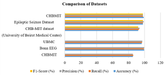
Figure 17. Model performance comparison on CHB-MIT [25] and Epileptic Seizure Dataset [24, 30, 31]
Figure 17 compares model performance on CHB-MIT and Epileptic Seizure Datasets using Accuracy, Precision, Recall, and F1-Score, with the latter outperforming across all metrics (88%–100%), showing its suitability. While the model achieves 98% accuracy on the clean, balanced Bonn EEG dataset [24], it may not reflect real-world complexity [30], potentially inflating results. Figure 12 suggests early validation loss convergence, indicating possible overfitting despite using dropout and SMOTE. The confusion matrix (Figure 11) shows 24 false positives and 15 false negatives, which in clinical settings could lead to missed or unnecessary interventions. Hence, further validation on diverse, multi-patient datasets is needed for clinical reliability [30, 31]. Table 4 compares the model's performance across multiple EEG datasets, showcasing consistently high accuracy and recall, with the Bonn EEG dataset yielding the best results.
5.3 Interpretation of SHAP output and neurophysiological correlation
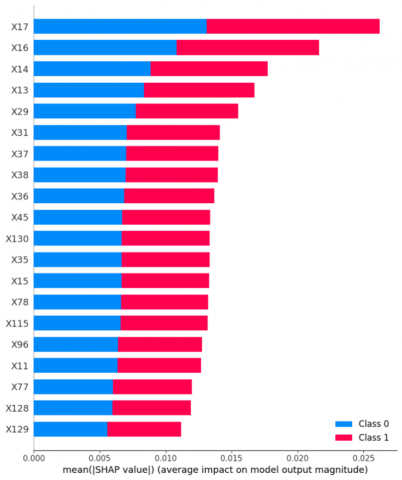
Figure 18 shows the impact of features X17 to X129 on model output using mean absolute SHAP values (x-axis). Each feature reflects its influence on Class 0 and Class 1 predictions. Longer bars indicate greater impact. This analysis enhances model interpretability and feature significance.
Figure 18. SHAP analysis function
The effects of attributes X17 through X77 on the results of a predictive model are shown in Figure 7. The average influence on the size of the model's output is shown by the mean absolute SHAP value on the x-axis. The effects of each characteristic, ranging from X17 to X77, on Class 0 and Class 1 predictions are indicated. Greater impact on model predictions or a higher mean SHAP value is indicated by longer bars.
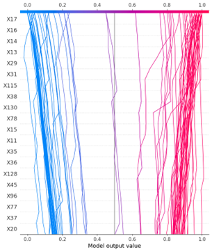
Figures 18 and 19 show SHAP outputs, clearly identifying the EEG features contributing most to classification. This interpretability enables clinicians to better understand the model’s decisions and supports its adoption in real-world healthcare.
Figure 19. SHAP model output
Figures 18 and 19 also present the SHAP analysis, offering insight into the contribution of individual EEG-derived features toward the prediction of epileptic seizures. Notably, features corresponding to channels X17, X22, X34, X46, X68, and X73 exhibited the highest SHAP values, indicating their substantial influence on the model’s output. These channels are predominantly associated with electrodes placed over the temporal and frontal brain regions—areas widely recognized in the epilepsy literature as common sites for seizure onset and propagation [6, 7, 17].
Temporal lobe structures are considered highly epileptogenic due to their involvement in the limbic system, which is frequently implicated in seizure initiation. Likewise, the frontal regions often demonstrate early spike-wave activity in focal seizures, further reinforcing the clinical relevance of these high-SHAP features [9].
With respect to frequency bands, the model leverages wavelet decomposition to extract multiscale frequency components, including high-frequency (cD3), mid-frequency (cD2), low-frequency (cD1), and approximation (cA1) bands. Among these, cD2 and cD3—corresponding to the beta (14–30 Hz) and gamma (>30 Hz) frequency ranges—showed significant SHAP values, highlighting their importance in seizure prediction. This finding is consistent with previous studies that report elevated beta and gamma power in the pre-ictal phase due to increased neuronal synchronization [21, 32].
Overall, the SHAP-based feature importance analysis validates not only the model’s predictive strength but also its alignment with well-established neurophysiological markers of epilepsy. By integrating model interpretability with domain knowledge, this approach enhances clinical credibility and contributes to the development of actionable decision-support systems for early seizure intervention.
The proposed Wavelet-CNN-LSTM model achieved 98% accuracy, 98% recall, and 98.7% precision (1798 TP, 24 FP; Figure 11), demonstrating strong potential for seizure prediction with superior accuracy and interpretability over previous methods. The pipeline comprises EEG data collection, normalization, Wavelet CNN for spatial-frequency feature extraction, and LSTM for capturing temporal dependencies. SHAP analysis enhances model transparency by highlighting key predictive features, enabling global and local interpretability. The model was evaluated using standard metrics and benchmarked against existing techniques. Although high accuracy was achieved on the Bonn EEG dataset, its artifact-free and balanced nature limits clinical generalizability [24]. The early plateau in validation loss (Figure 13) indicates potential overfitting. Despite applying dropout and SMOTE, further validation using complex datasets such as CHB-MIT [25], UBMC [17], and TUH EEG is necessary to ensure robustness across real-world conditions.
Clinically, the model shows promise with a low false positive rate (1.3%) and high recall (98%), ensuring minimal missed seizures, which is crucial for patient safety. This effective balance between sensitivity and specificity supports reliable and ethically responsible deployment. SHAP-driven insights improve clinical trust by revealing EEG features influencing predictions, helping physicians make informed treatment decisions and enabling more personalized care. While the model is computationally intensive and depends on high-quality labeled data, its ability to capture spatial, temporal, and frequency-domain patterns positions it as a viable tool for seizure prediction and broader medical time-series analysis.
This study presents a novel and interpretable deep learning framework for early prediction of epileptic seizures using EEG data. By integrating Wavelet-based CNN for spatial-frequency feature extraction, LSTM for capturing temporal patterns, and SHAP for interpretability, the model achieved 98% accuracy, 98% recall, and 98.7% precision on the Bonn EEG dataset. These results demonstrate the model’s robustness and clinical relevance.
Future work will involve:
By enhancing both predictive performance and transparency, this approach contributes meaningfully toward practical, explainable AI solutions in neurodiagnostics.
[1] Huang, X., Sun, X., Zhang, L., Zhu, T., Yang, H., Xiong, Q., Feng, L. (2022). A novel epilepsy detection method based on feature extraction by deep autoencoder on EEG signal. International Journal of Environmental Research and Public Health, 19(22): 15110. https://doi.org/10.3390/ijerph192215110
[2] Jevin, M.J., Jayant, H., Sanjay, R., Hemasai, V., Venkatasrinivas, P.V. (2023). Heart disease identification method using machine learning classification in e-healthcare. International Journal of Advanced Research in Arts, Science, Engineering & Management, 10(3): 2322-2327.
[3] Li, J.P., Haq, A.U., Din, S.U., Khan, J., Khan, A., Saboor, A. (2020). Heart disease identification method using machine learning classification in e-healthcare. IEEE Access, 8: 107562-107582. https://doi.org/10.1109/ACCESS.2020.3001149
[4] Wei, L., Mooney, C. (2023). Transfer learning-based seizure detection on multiple channels of paediatric EEGs. In 2023 45th Annual International Conference of the IEEE Engineering in Medicine & Biology Society (EMBC), Sydney, Australia, pp. 1-4. https://doi.org/10.1109/EMBC40787.2023.10340210
[5] Ahmad, I., Yao, C., Li, L., Chen, Y., Liu, Z., Ullah, I., Chen, S. (2024). An efficient feature selection and explainable classification method for EEG-based epileptic seizure detection. Journal of Information Security and Applications, 80: 103654. https://doi.org/10.1016/j.jisa.2023.103654
[6] Sánchez-Hernández, S.E., Torres-Ramos, S., Román-Godínez, I., Salido-Ruiz, R.A. (2024). Evaluation of the relation between Ictal EEG features and XAI explanations. Brain Sciences, 14(4): 306. https://doi.org/10.3390/brainsci14040306
[7] Chung, Y.G., Jeon, Y., Yoo, S., Kim, H., Hwang, H. (2021). Big data analysis and artificial intelligence in epilepsy–common data model analysis and machine learning-based seizure detection and forecasting. Clinical and Experimental Pediatrics, 65(6): 272-282. https://doi.org/10.3345/cep.2021.00766
[8] İnce, R., Adanır, S.S., Sevmez, F. (2021). The inventor of electroencephalography (EEG): Hans Berger (1873–1941). Child's Nervous System, 37(9): 2723-2724. https://doi.org/10.1007/s00381-020-04564-z
[9] Rashed-Al-Mahfuz, M., Moni, M.A., Uddin, S., Alyami, S.A., Summers, M.A., Eapen, V. (2021). A deep convolutional neural network method to detect seizures and characteristic frequencies using epileptic electroencephalogram (EEG) data. IEEE Journal of Translational Engineering in Health and Medicine, 9: 1-12. https://doi.org/10.1109/JTEHM.2021.3050925
[10] Jonna, S.T., Natarajan, K. (2025). EEG signal processing in neurological conditions using machine learning and deep learning methods: A comprehensive review. The European Physical Journal Special Topics, pp. 1-19. https://doi.org/10.1140/epjs/s11734-025-01606-y
[11] Vieira, J.C., Guedes, L.A., Santos, M.R., Sanchez-Gendriz, I. (2023). Using explainable artificial intelligence to obtain efficient seizure-detection models based on electroencephalography signals. Sensors, 23(24): 9871. https://doi.org/10.3390/s23249871
[12] Chowdhury, B.R., Chowdhury, L. (2022). Explaining decisions of quantum algorithm: Patient specific features explanation for epilepsy disease. In Data-Driven Approach for Bio-medical and Healthcare, pp. 63-81. https://doi.org/10.1007/978-981-19-5184-8_4
[13] Zhang, X., Yao, L., Dong, M., Liu, Z., Zhang, Y., Li, Y. (2020). Adversarial representation learning for robust patient-independent epileptic seizure detection. IEEE Journal of Biomedical and Health Informatics, 24(10): 2852-2859. https://doi.org/10.1109/JBHI.2020.2971610
[14] Lo Giudice, M., Varone, G., Ieracitano, C., Mammone, N., Tripodi, G.G., Ferlazzo, E., Morabito, F.C. (2022). Permutation entropy-based interpretability of convolutional neural network models for interictal EEG discrimination of subjects with epileptic seizures vs. psychogenic non-epileptic seizures. Entropy, 24(1): 102. https://doi.org/10.3390/e24010102
[15] Al-Hussaini, I., Mitchell, C.S. (2023). SeizFt: Interpretable machine learning for seizure detection using wearables. Bioengineering, 10(8): 918. https://doi.org/10.3390/bioengineering10080918
[16] Hussein, R., Lee, S., Ward, R., McKeown, M.J. (2021). Semi-dilated convolutional neural networks for epileptic seizure prediction. Neural Networks, 139: 212-222. https://doi.org/10.1016/j.neunet.2021.03.008
[17] Raab, D., Theissler, A., Spiliopoulou, M. (2023). XAI4EEG: Spectral and spatio-temporal explanation of deep learning-based seizure detection in EEG time series. Neural Computing and Applications, 35(14): 10051-10068. https://doi.org/10.1007/s00521-022-07809-x
[18] Ludwig, S.A. (2022). Explainability using SHAP for epileptic seizure recognition. In 2022 IEEE International Conference on Big Data (Big Data), Osaka, Japan, pp. 5305-5311. https://doi.org/10.1109/BigData55660.2022.10021103
[19] Bijoy, E.H., Rahman, M.H., Ahmed, S., Laskor, M.S. (2022). An approach to detect epileptic seizure using XAI and machine learning. PhD Thesis, Brac University.
[20] Wei, L., Mooney, C. (2023). Investigating the need for pediatric-specific machine learning approaches for seizure detection in EEG. In 2023 11th International Conference on Bioinformatics and Computational Biology (ICBCB), Hangzhou, China, pp. 57-63. https://doi.org/10.1109/ICBCB57893.2023.10246719
[21] Akut, R. (2019). Wavelet based deep learning approach for epilepsy detection. Health Information Science and Systems, 7(1): 8. https://doi.org/10.1007/s13755-019-0069-1
[22] Wang, F., Yu, Y., Zhang, Z., Li, J., Zhen, Z., Li, K. (2018). Wavelet decomposition and convolutional LSTM networks based improved deep learning model for solar irradiance forecasting. Applied Sciences, 8(8): 1286. https://doi.org/10.3390/app8081286
[23] Ibrahim, F.E., Emara, H.M., El-Shafai, W., Elwekeil, M., Rihan, M., Eldokany, I.M., Abd El-Samie, F.E. (2022). Deep-learning-based seizure detection and prediction from electroencephalography signals. International Journal for Numerical Methods in Biomedical Engineering, 38(6): e3573. https://doi.org/10.1002/cnm.3573
[24] Shakir, Y.H. (2021). Epileptic seizure recognition. https://www.kaggle.com/datasets/yasserhessein/epileptic-seizure-recognition.
[25] Gotoh, M. (2023). CHB-MIT eeg dataset: Seizure detection demo. https://www.kaggle.com/code/masahirogotoh/chb-mit-eeg-dataset-seizure-detection-demo.
[26] Tsiouris, K.M., Pezoulas, V.C., Koutsouris, D.D., Zervakis, M., Fotiadis, D.I. (2017). Discrimination of preictal and interictal brain states from long-term EEG data. In 2017 IEEE 30th International Symposium on Computer-Based Medical Systems (CBMS), Thessaloniki, Greece, pp. 318-323. https://doi.org/10.1109/CBMS.2017.33
[27] Elgohary, S., Eldawlatly, S., Khalil, M.I. (2016). Epileptic seizure prediction using zero-crossings analysis of EEG wavelet detail coefficients. In 2016 IEEE Conference on Computational Intelligence in Bioinformatics and Computational Biology (CIBCB), Chiang Mai, Thailand, pp. 1-6. https://doi.org/10.1109/CIBCB.2016.7758115
[28] Wang, H., Shi, W., Choy, C.S. (2018). Hardware design of real time epileptic seizure detection based on STFT and SVM. IEEE Access, 6: 67277-67290. https://doi.org/10.1109/ACCESS.2018.2870883
[29] Ibrahim, S.W., Djemal, R., Alsuwailem, A., Gannouni, S. (2017). Electroencephalography (EEG)-based epileptic seizure prediction using entropy and K-nearest neighbor (KNN). Communications in Science and Technology, 2(1): 6-10. https://doi.org/10.21924/cst.2.1.2017.44
[30] Gabeff, V., Teijeiro, T., Zapater, M., Cammoun, L., Rheims, S., Ryvlin, P., Atienza, D. (2021). Interpreting deep learning models for epileptic seizure detection on EEG signals. Artificial Intelligence in Medicine, 117: 102084. https://doi.org/10.1016/j.artmed.2021.102084
[31] Halimeh, M., Jackson, M., Vieluf, S., Loddenkemper, T., Meisel, C. (2023). Explainable AI for wearable seizure logging: Impact of data quality, patient age, and antiseizure medication on performance. Seizure: European Journal of Epilepsy, 110: 99-108. https://doi.org/10.1016/j.seizure.2023.06.002
[32] Song, K., Fang, J., Zhang, L., Chen, F., Wan, J., Xiong, N. (2022). An intelligent epileptic prediction system based on synchrosqueezed wavelet transform and multi-level feature CNN for smart healthcare IoT. Sensors, 22(17): 6458. https://doi.org/10.3390/s22176458