Arjun Bhavadharani![]() | Dickson Kamala Sheena Christy*
| Dickson Kamala Sheena Christy*![]()
© 2025 The authors. This article is published by IIETA and is licensed under the CC BY 4.0 license (http://creativecommons.org/licenses/by/4.0/).
OPEN ACCESS
Cellular Automata serve as powerful tools for modeling dynamic processes in real-world systems. The geometric structure of a cellular automaton directly influences its algebraic properties, which are governed by the underlying local transition rules. In this work, we explore the algebraic structure of finite linear Triangular Lattice Moore Cellular Automata under null boundary conditions. The Moore neighborhood of a triangular lattice includes 13 neighbors at radius 1. We construct the rule matrices for finite linear Triangular Lattice Moore Cellular Automata under null boundary condition. We present an algorithm for the pattern evolution of such automata and observe the emergence of intricate patterns such as hexagonal fractals and radially symmetric structures. These patterns are characterized by recursive growth making them suitable for applications in algorithmic art, digital textiles, and architectural tiling. Reversibility in two-dimensional Cellular Automata is difficult to determine due to complex neighborhood interactions. By constructing rule matrices, we provide an algebraic framework that enables the decidability of the reversibility and retrieval of previous configurations. This framework offers a systematic approach to study reversibility in complex lattice structures, laying the foundation for further theoretical and applied research in finite linear Triangular Lattice Moore Cellular Automata.
Cellular Automata, triangular lattice, Moore neighborhood, null boundary, matrix algebra, fractals
The interrelationship between elements of a system greatly influences its behavior. From the mid-20th century, various scientists started proposing multiple models for this approach. Cellular Automata (CA) is one of the magnificent models scientists welcome in this direction of study. Cellular Automata is a discrete model of computation that plays a significant role in the simulation of real-world systems. In 1996, von Neumann and Burks [1] initiated the concept of CA by modeling self-reproduction in biological systems. CA is modeled with a grid of cells that evolve over discrete generations depending upon the local transition rules. The major factors influencing the evolution of two-dimensional cellular automaton is the lattice shape, type of neighborhood, the set of states and the nature of the local transition rule. Cellular Automata rules can be categorized into two main classifications: linear rules and non - linear rules. The majority of research in Cellular Automata has focused on one-dimensional models where the lattice shape is not a critical factor. However, in two-dimensional Cellular Automata, the geometry of the underlying lattice significantly influences the system's dynamics and evolution. In this context, researchers have extended traditional square lattice models to explore more complex topologies such as hexagonal and triangular lattices. These alternative lattice structures introduce different neighborhood configurations, which directly affect rule formulation, propagation behavior, and pattern formation. Notable studies have examined the impact of such lattice variations on Cellular Automata behavior, particularly in modeling natural systems, pattern generation, and computational complexity.
The choice of lattice geometry such as square, triangular [2], hexagonal [3, 4], or pentagonal [5] significantly influences neighborhood configurations and consequently the system's evolution. Triangular grids produce certain shapes and patterns that are not possible to achieve with the typical square grid CA. Zawidzki [6] introduced the concept of Cellular Automata on a triangular tessellation. Saadat and Nagy [7, 8] and Morita [9] examined the approach of Cellular Automata on a triangular grid. One major factor of a Cellular Automata is the type of neighborhood considered. John von Neumann proposed a neighborhood model that depends on the current cell and its adjacent cells. In 1962, Moore [10] proposed an extended form of the neighborhood proposed by von Neumann. In this case, the neighborhood depends upon the center cell, its adjacent cells, and the cells connected with the nodes of the center cell. The Moore neighborhood of the triangular lattice consists 13 neighbors which is the highest of any other lattice for neighborhood of radius 1.
The geometric structure of Cellular Automata promotes curiosity about decoding the algebraic characterization behind the automata. A finite Cellular Automata comprises of a finite number of cells, each mapping to a state. A specific local transition rule computes each cell state at the next generation. A concise and clear representation of the rules using mathematical logic aids in understanding how the automata compute the next generation. Das et al. [11, 12], Ganguly et al. [13], and Pal Chaudhuri et al. [14] characterized the behavior of CA’s state transition using matrix algebra. The work by Kaspar et al. [15] on two-dimensional automata laid the motivation to explore the properties of two-dimensional Cellular Automata. Two-dimensional CAs, due to their variety of purposes, are investigated by Packard and Wolfram [16], Terrier [17], Durand [18], de Oliveira et al. [19], Kari [20], and many others. References [21-26] investigated the algebraic properties of two-dimensional CA using matrix algebra.
In infinite Cellular Automata, boundary conditions are inherently absent, and thus have no influence on the system's evolution. However, in finite Cellular Automata, boundary conditions become integral to the dynamics, as they directly affect the evolution of configurations over time. The interaction between the finite grid and its boundaries can lead to emergent behaviors that significantly impact the global evolution of the system. The two most prevalent boundary conditions are the null and periodic boundaries and their effects can be explored from the study of LuValle [27]. The work by Sahin et al. [28] explores the various boundary conditions of two-dimensional Cellular Automata using von Neumann neighborhood. In this work, we consider the finite Cellular Automata in a two-dimensional grid on a triangular lattice. In 2017, Uguz et al. [29] examined the reversibility and structure of the linear, triangular, two-dimensional von Neumann Cellular Automata with null boundary condition. However, in their formulation, the current (center) cell was not included as part of the neighborhood and was therefore excluded from the rule matrix construction. This omission deviates from the conventional CA framework, where the current cell is typically considered an essential part of the neighborhood. In the present work, we address this limitation by explicitly incorporating the center cell into the neighborhood definition and the corresponding rule matrix.
Triangular lattice Cellular Automata are known for their ability to generate aesthetically pleasing and highly symmetric patterns that are often difficult to replicate using square or hexagonal lattices. The inherent angular structure and rotational symmetry of the triangular grid allows for intricate interlocking motifs, radial formations, and fractal-like growth that are naturally aligned with equilateral geometry. These properties make triangular lattices particularly well-suited for visual complexity and symmetry, often resembling traditional tessellations and decorative art. The triangular lattice has gained significant attention in recent Cellular Automata research due to its geometric versatility and ability to generate complex, symmetric patterns which are not easily achievable with traditional square grids. Saadat and Nagy [8] further illustrated the expressive potential of triangular lattice Cellular Automata by generating intricate patterns like mandalas and trees through alternating rule applications. Ray et al. [30] utilized probabilistic Cellular Automata on two-dimensional structures to preserve quantum information, showing how lattice geometry influences memory stability under noise. Verhodubs [31] combined ontological frameworks with Cellular Automata to simulate cognitive processes, leveraging triangular lattices for spatial efficiency in representing thought dynamics.
The Moore neighborhood on a triangular lattice is more complicated than those on square and hexagonal lattices because it has more neighbors and different ways they interact. Despite its rich dynamics, the algebraic characterization of Triangular Lattice Moore Cellular Automata (TLMCA) remains largely unexplored in the current literature. This research aims to fill that gap by creating a way to represent the rules of how these automata change both locally and globally using a matrix. By using matrix algebra, we can break down the complicated local connections, making it easier to analyze the overall rule structure. This approach simplifies the complexity and opens a path to examine the reversibility.
In this work, we study the algebraic structure of finite linear TLMCA under null boundary condition. We consider the Moore neighborhood under null boundary condition. The structure of the paper is as follows: Section 2 provides some basic definitions. The rule matrix for finite linear TLMCA with null boundary condition is given in Section 3. In Section 4, we provided a method to find the $s^{th}$ configuration from the $s+1^{t h}$ configuration of the finite linear TLMCA with null boundary condition. Also presented an algorithm to generate patterns with finite linear TLMCA and the patterns generated using finite linear TLMCA in Section 4. The illustration of the pattern evolution and rule matrix evolution is presented in Section 5.
The basic definitions of CA are recalled in this section. To explore more about the fundamentals of CA, refer to the lecture notes by Kari [32].
Definition 1. A Cellular Automata is stated as a quadruple ($L, Q, N, F$), where, $L \subseteq Z^m$ is the $m$-dimensional lattice, $Q$ is the finite set of states, $N=\left(v_1, v_2, \ldots, v_n\right)$ is the set of neighborhood vectors of distinct states of $L, f: Q^p \rightarrow Q$ is the local transition rule [33].
This work deals with two-dimensional triangular lattice with Moore neighborhood. The value p denotes the number of neighbors. In triangular lattice Cellular Automata with Moore neighborhood, we have n=13.
Definition 2. A configuration of the $m$-dimensional Cellular Automata with state set $Q$ is defined by the mapping $C: Z^m \rightarrow Q$ where $Z^m$ is a $m$-dimensional lattice and $Q$ is the finite set of states [23].
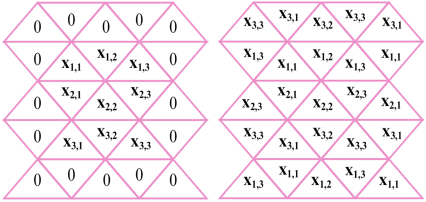
Each $(i, j)^{\text {th }}$ element in $Z^m$ is labelled as $x_{i, j}$. The configuration of the two-dimensional Cellular Automata is represented by a matrix of order $\mathrm{m} \times \mathrm{n}$. The configuration at time ' $s$ ' is
$\mathrm{C}^{(\mathrm{s})}=\left(\begin{array}{ccc}v_{1,1}^{(\mathrm{s})} & \cdots & v_{1, \mathrm{n}}^{(\mathrm{s})} \\ \vdots & \ddots & \vdots \\ v_{\mathrm{m}, 1}^{(\mathrm{s})} & \cdots & v_{\mathrm{m}, \mathrm{n}}^{(\mathrm{s})}\end{array}\right)$
where, $v_{i, j}^{(s)}$ represents the state of each cell $x_{i, j}$ at time 's'.
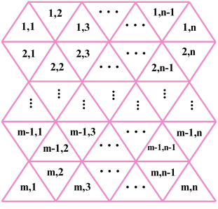
The $m \times n$ (m rows and in columns) arrangement of lattice points for a two-dimensional finite triangular lattice is explained in Figure 1.
Figure 1. $m \times n$ triangular lattice
Definition 3. von Neumann Neighborhood put forth by von Neumann is two-dimensional and relies on 4 neighborhood dependency, including the center cell and its adjacent ones [1].
For the triangular lattice Cellular Automata there are two types of von Neumann neighborhood dependencies.
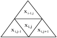
If the cell $x_{i,j}$ lies inside the upward triangle (Figure 2), the neighborhood vector is given by
$\left(x_{i, j}, x_{i, j+1}, x_{i+1, j}, x_{i, j-1}\right)$
Figure 2. von Neumann neighborhood configuration of the cell $x_{i,j}$ to be inside upright triangle
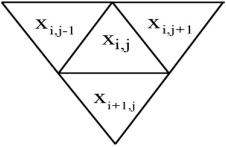
If the cell $x_{i,j}$ lies inside the inverted triangle (Figure 3), the neighborhood vector is given by
$\left(x_{i, j}, x_{i-1, j}, x_{i, j+1}, x_{i, j-1}\right)$
Figure 3. von Neumann neighborhood configuration of the cell $x_{i,j}$ to be inside inverted triangle
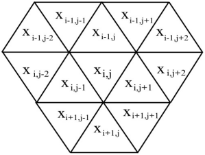
Definition 4. Moore Neighborhood is the extended neighborhood dependency of von Neumann neighborhood, in which neighborhood depends on adjacent cells and the cells connected to the nodes of the center cell (Figure 4 and Figure 5) [10].
Figure 4. Moore neighborhood configuration of the cell $x_{i,j}$ to be inside upright triangle
Figure 5. Moore neighborhood configuration of the cell $x_{i,j}$ to be inside inverted triangle
Definition 5. The case where the cells on the boundary are connected to 0 logic state is known as null boundary Cellular Automata [27].
Table 1 represents the 3 × 3 null boundary CA where each $v_{i,j}$ represents the state of the corresponding cell $x_{i,j}$. Table 2 represents the 3 × 3 periodic boundary cellular automaton.
Table 1. A 3 × 3 null boundary CA
|
0 |
0 |
0 |
0 |
0 |
|
0 |
νi−1,j−1 |
νi−1,j |
νi−1,j+1 |
0 |
|
0 |
νi,j−1 |
νi,j |
νi,j+1 |
0 |
|
0 |
νi+1,j−1 |
νi+1,j |
νi+1,j+1 |
0 |
|
0 |
0 |
0 |
0 |
0 |
Table 2. A 3 × 3 periodic boundary CA
|
νi−1,j−1 |
νi−1,j |
νi+1,j |
νi+1,j+1 |
νi+1,j−1 |
|
νi−1,j+1 |
νi−1,j−1 |
νi−1,j |
νi−1,j+1 |
νi−1,j−1 |
|
νi,j+1 |
νi,j−1 |
νi,j |
νi,j+1 |
νi,j−1 |
|
νi+1,j+1 |
νi+1,j−1 |
νi+1,j |
νi+1,j+1 |
νi+1,j−1 |
|
νi−1,j+1 |
νi−1,j−1 |
νi−1,j |
νi−1,j+1 |
νi−1,j−1 |
(a) (b)
Figure 6. (a) Null boundary; (b) Periodic boundary
Definition 6. The case where the extreme cells are next to one another is known as periodic boundary Cellular Automata.
Figure 6(a) and Figure 6(b) depict the mapping of cells based on boundary conditions for a finite 3×3 CA [27].
This section defines the Moore neighborhood and associated linear transition rule for a cell in a triangular lattice. Let $r\left(v_{i, j}\right)$ be the transition rule for each cell in the triangular lattice. The transition rule is defined in two distinct ways due to the presence of two categories of neighborhood states, which are determined by the position of the triangle (upward and downward). This finite linear TLMCA deals with finite number of states. We consider ternary state set throughout this work.
Definition 7. Moore neighborhood of a triangular lattice Cellular Automata is defined as a 13 − tuple.
If the cell $x_{i, j}$ lies inside the inverted triangle, then the neighborhood vector is defined as
$\begin{aligned} & \left(v_{i, j}, v_{i-1, j}, v_{i, j+1}, v_{i, j-1}, v_{i-1, j+1}, v_{i-1, j+2}, v_{i, j+2}\right.,\left.v_{i+1, j+1}, v_{i+1, j}, v_{i+1, j-1}, v_{i, j-2}, v_{i-1, j-2}, v_{i-1, j-1}\right)\end{aligned}$
If the cell $x_{i, j}$ lies inside the upright triangle, then the neighborhood vector is defined as
$\begin{aligned} & \left(v_{i, j}, v_{i, j+1}, v_{i+1, j}, v_{i, j-1}, v_{i, j+2}, v_{i+1, j+2}, v_{i+1, j+1},\right.\left.v_{i+1, j-1}, v_{i+1, j-2}, v_{i, j-2}, v_{i-1, j-1}, v_{i-1, j}, v_{i-1, j+1}\right)\end{aligned}$
where, each $v_{i, j}$ represents the state of the cell $x_{i, j}$.
Definition 8. Local transition rule of the finite linear TLMCA is defined as $R: C^t \rightarrow C^{t+1}$ where $R=\left\{r\left(v_{i, j}\right)\right\} . v_{i, j}$ represents the state of the cell $x_{i, j}$.
If $v_{i, j}$ lies inside the inverted triangle
$\begin{aligned} r\left(v_{i, j}\right)=\left(a_0 v_{i, j}+\right. & a v_{i-1, j}+b v_{i, j+1}+c v_{i, j-1}+a_1 v_{i-1, j+1}+a_2 v_{i-1, j+2}+a_3 v_{i, j+2}+b_1 v_{i+1, j+1} \\ & +b_2 v_{i+1, j}+b_3 v_{i+1, j-1}+c_1 v_{i, j-2}\left.+c_2 v_{i-1, j-2}+c_3 v_{i-1, j-1}\right) \bmod 3\end{aligned}$ (1)
If $v_{i, j}$ lies inside the upright triangle
$\begin{gathered}r\left(v_{i, j}\right)=\left(d_0 v_{i, j}+d v_{i, j+1}+e v_{i+1, j}+f v_{i, j-1}+\right.d_1 v_{i, j+2}+d_2 v_{i+1, j+2}+d_3 v_{i+1, j+1}+e_1 v_{i+1, j-1}+ \\ e_2 v_{i+1, j-2}+e_3 v_{i, j-2}+f_1 v_{i-1, j-1}+f_2 v_{i-1, j}+\left.f_3 v_{i-1, j+1}\right) \bmod 3\end{gathered}$ (2)
where,
$\begin{gathered}a_0, b, c, a_1, a_2, a_3, b_1, b_2, b_3, c_1, c_2, c_3, d_0, e, f, d_1, d_2, d_3, e_1, e_2, e_3, f_1, f_2, f_3 \in Z_k\end{gathered}$
Definition 9. A finite linear TLMCA is defined as a quadruple $T_M=(L, Q, N, R)$ where, $L$ is a two-dimensional triangular lattice $L \subseteq Z^2, Q$ is the finite set of states denoted by $v_{i, j}, N$ is the set of all 13-tuple neighborhood vectors $\left(n_1, n_2, \ldots, n_{13}\right)$ for all $m \cdot n$ cells of the triangular lattice Cellular Automata and $R$ is the local transition rule $R: C^{(s)} \rightarrow C^{(s+1)}$ and $R=\left\{r\left(v_{i, j}\right)\right\}$.
The rule matrices for obtaining the next step configurations of finite linear TLMCA are derived in the following theorems.
Theorem 1. Let $T_M$ be a finite linear TLMCA under null boundary condition over the field $Z_3$. Then the rule matrix of order $m \times m$ which updates the $s^{\text {th }}$ finite linear TLMCA configuration $C^{(s)}$ to $(s+1)^{\text {th }}$ configuration $C^{(s+1)}$ is given by
$\mathcal{T}_{\mathcal{R}}^{\mathcal{O}\mathcal{O}}=\left(\begin{array}{ccccccc}\alpha_1 & \beta_1 & \mathcal{O} & & \mathcal{O} & \mathcal{O} & \mathcal{O} \\ \gamma_1 & \alpha_2 & \beta_2 & \cdots & \mathcal{O} & \mathcal{O} & \mathcal{O} \\ \mathcal{O} & \gamma_2 & \alpha_1 & & \mathcal{O} & \mathcal{O} & \mathcal{O} \\ & \vdots & & \ddots & & \vdots & \\ \mathcal{O} & \mathcal{O} & \mathcal{O} & & \alpha_1 & \beta_1 & \mathcal{O} \\ \mathcal{O} & \mathcal{O} & \mathcal{O} & \cdots & \gamma_1 & \alpha_2 & \beta_2 \\ \mathcal{O} & \mathcal{O} & \mathcal{O} & & \mathcal{O} & \gamma_2 & \alpha_1\end{array}\right)$
where, $\alpha_1, \alpha_2, \beta_1, \beta_2, \gamma_1, \gamma_2$ are $n \times n$ submatrices and $\mathcal{O}$ is an $n \times n$ null matrix. Here $m$ and $n$ are odd positive integers.
Proof. Let $T_M=(L, Q, N, R)$ be the finite linear TLMCA. $L$ is an $m \times n$ two-dimensional triangular lattice where $m$ and $n$ are odd positive integers. $Q$ is the finite set of states. Let us consider the cellular automaton has 3 states $\{0,1,2\} . N$ is the set neighborhood vectors. $R$ is the set of local transition rules. $R$ is defined as $R: C^{(s)} \rightarrow C^{(s+1)}$ where $R=\left\{r\left(v_{i, j}\right)\right\}$.
If $v_{i, j}$ lies inside the inverted triangle, from Eq. (1)
$\begin{gathered}r\left(v_{i, j}\right)=\left(a_0 v_{i, j}+a v_{i-1, j}+b v_{i, j+1}+c v_{i, j-1}+\right.a_1 v_{i-1, j+1}+a_2 v_{i-1, j+2}+a_3 v_{i, j+2} \\ +b_1 v_{i+1, j+1}+b_2 v_{i+1, j}+\left.b_3 v_{i+1, j-1}+c_1 v_{i, j-2}+c_2 v_{i-1, j-2}+c_3 v_{i-1, j-1}\right) \bmod 3\end{gathered}$
If $v_{i, j}$ lies inside the upright triangle, from Eq. (2)
$\begin{gathered}r\left(v_{i, j}\right)=\left(d_0 v_{i, j}+d v_{i, j+1}+e v_{i+1, j}+f v_{i, j-1}+d_1 v_{i, j+2}+\right.d_2 v_{i+1, j+2}+d_3 v_{i+1, j+1} \\+e_1 v_{i+1, j-1} +e_2 v_{i+1, j-2}+\left.e_3 v_{i, j-2}+f_1 v_{i-1, j-1}+f_2 v_{i-1, j}+f_3 v_{i-1, j+1}\right) \bmod 3\end{gathered}$
where,
$\begin{gathered}a_0, b, c, a_1, a_2, a_3, b_1, b_2, b_3, c_1, c_2, c_3, d_0, e, f, d_1, d_2, d_3, e_1, e_2, e_3, f_1, f_2, f_3 \in Z_k\end{gathered}$
Let $v_{i, j}=0 \quad$ when $i \notin\{1,2, \cdots m\}$ or $j \notin\{1,2, \cdots n\}$ because of employing null boundary conditions. By applying the local transition rule from Eqs. (1) and (2) to each cell in the automata, $m \cdot n$ linear equations are obtained.
$\begin{aligned} r\left(v_{1,1}\right)=\left(d_0 v_{1,1}\right. & +d v_{1,2}+e v_{2,1}+f v_{1,0}+d_1 v_{1,3}+d_2 v_{2,3}+d_3 v_{2,2} \\ &+e_1 v_{2,0} +e_2 v_{2,-1}+e_3 v_{1,-1}+f_1 v_{0,0}\left.+f_2 v_{0,1}+f_3 v_{0,2}\right) \bmod 3\end{aligned}$ (3)
$\begin{aligned} r\left(v_{1,2}\right)=\left(a_0 v_{1,2}\right. & +a v_{0,2}+b v_{1,3}+c v_{1,1}+a_1 v_{0,3}+a_2 v_{0,4}+a_3 v_{1,4}+b_1 v_{2,3} \\ & +b_2 v_{2,2}+b_3 v_{2,1}+c_1 v_{1,0}+c_2 v_{0,0}\left.+c_3 v_{0,1}\right) \bmod 3\end{aligned}$ (4)
$\begin{aligned} r\left(v_{1, n}\right)=\left(d_0 v_{1, n}\right. & +d v_{1, n+1}+e v_{2, n}+f v_{1, n-1}+d_1 v_{1, n+2}+d_2 v_{2, n+2}+d_3 v_{2, n+1} \\ & +e_1 v_{2, n-1}+e_2 v_{2, n-2}+e_3 v_{1, n-2}+f_1 v_{0, n-1}+f_2 v_{0, n}\left.+f_3 v_{0, n+1}\right) \bmod 3\end{aligned}$ (5)
$\begin{aligned} r\left(v_{2,1}\right)=\left(a_0 v_{2,1}\right. & +a v_{1,1}+b v_{2,2}+c v_{2,0}+a_1 v_{1,2}+a_2 v_{1,3}+a_3 v_{2,3}+b_1 v_{3,2} \\ & +b_2 v_{3,1}+b_3 v_{3,0}+c_1 v_{2,-1}\left.+c_2 v_{1,-1}+c_3 v_{1,0}\right) \bmod 3\end{aligned}$ (6)
$\begin{aligned} r\left(v_{2,2}\right)=\left(d_0 v_{2,2}\right. & +d v_{2,3}+e v_{3,2}+f v_{2,1}+d_1 v_{2,4}+d_2 v_{3,4}+d_3 v_{3,3} \\ & +e_1 v_{3,1}+e_2 v_{3,0}+e_3 v_{2,0}+f_1 v_{1,1}\left.+f_2 v_{1,2}+f_3 v_{1,3}\right) \bmod 3\end{aligned}$ (7)
$\begin{aligned} r\left(v_{2, n}\right)=\left(a_0 v_{2, n}\right. & +a v_{1, n}+b v_{2, n+1}+c v_{2, n-1}+a_1 v_{1, n+1}+a_2 v_{1, n+2}+a_3 v_{2, n+2} \\ & +b_1 v_{3, n+1}+b_2 v_{3, n}+b_3 v_{3, n-1}+c_1 v_{2, n-2}+c_2 v_{1, n-2}\left.+c_3 v_{1, n-1}\right) \bmod 3\end{aligned}$ (8)
$\begin{aligned} r\left(v_{m, 1}\right)=\left(d_0 v_{m, 1}\right. & +d v_{m, 2}+e v_{m+1,1}+f v_{m, 0}+d_1 v_{m, 3}+d_2 v_{m+1,3}+d_3 v_{m+1,2}+e_1 v_{m+1,0} \\ & +e_2 v_{m+1,-1}+e_3 v_{m,-1} +f_1 v_{m-1,0}+f_2 v_{m-1,1}\left.+f_3 v_{m-1,2}\right) \bmod 3\end{aligned}$ (9)
$\begin{aligned} r\left(v_{m, 2}\right)=\left(a_0 v_{m, 2}\right. & +a v_{m-1,2}+b v_{m, 3}+c v_{m, 1}+a_1 v_{m-1,3}+a_2 v_{m-1,4}+a_3 v_{m, 4}+b_1 v_{m+1,3} \\ & +b_2 v_{m+1,2}+b_3 v_{m+1,1}+c_1 v_{m, 0}+c_2 v_{m-1,0}\left.+c_3 v_{m-1,1}\right) \bmod 3\end{aligned}$ (10)
$\begin{aligned} r\left(v_{m, n}\right)=\left(d_0 v_{m, n}\right. & +d v_{m, n+1}+e v_{m+1, n}+f v_{m, n-1}+d_1 v_{m, n+2}+d_2 v_{m+1, n+2}+d_3 v_{m+1, n+1} +e_1 v_{m+1, n-1}\\ & +e_2 v_{m+1, n-2}+e_3 v_{m, n-2}+f_1 v_{m-1, n-1}+f_2 v_{m-1, n} \left.+f_3 v_{m-1, n+1}\right) \bmod 3\end{aligned}$ (11)
These equations can be represented in matrix form as:
$\mathcal{J}_{\mathcal{R}}^{\mathcal{O} \mathcal{O}}=\left(\begin{array}{ccccccc}\alpha_1 & \beta_1 & \mathcal{O} & & \mathcal{O} & \mathcal{O} & \mathcal{O} \\ \gamma_1 & \alpha_2 & \beta_2 & \cdots & \mathcal{O} & \mathcal{O} & \mathcal{O} \\ \mathcal{O} & \gamma_2 & \alpha_1 & & \mathcal{O} & \mathcal{O} & \mathcal{O} \\ & \vdots & & \ddots & & \vdots & \\ \mathcal{O} & \mathcal{O} & \mathcal{O} & & \alpha_1 & \beta_1 & \mathcal{O} \\ \mathcal{O} & \mathcal{O} & \mathcal{O} & \cdots & \gamma_1 & \alpha_2 & \beta_2 \\ \mathcal{O} & \mathcal{O} & \mathcal{O} & & \mathcal{O} & \gamma_2 & \alpha_1\end{array}\right)$
where,
$\alpha_1=\left(\begin{array}{ccccccccc}\mathrm{d}_0 & \mathrm{~d} & \mathrm{~d}_1 & 0 & 0 & & 0 & 0 & 0 \\ \mathrm{c} & \mathrm{a}_0 & \mathrm{~b} & \mathrm{a}_3 & 0 & & 0 & 0 & 0 \\ \mathrm{e}_3 & \mathrm{f} & \mathrm{d}_0 & \mathrm{~d} & \mathrm{~d}_1 & \cdots & 0 & 0 & 0 \\ 0 & \mathrm{c}_1 & \mathrm{c} & 0 & \mathrm{~b} & & 0 & 0 & 0 \\ 0 & 0 & \mathrm{e}_3 & \mathrm{f} & \mathrm{d}_0 & & 0 & 0 & 0 \\ & & \vdots & & & \ddots & & \vdots & \\ 0 & 0 & 0 & 0 & 0 & & \mathrm{~d}_0 & \mathrm{~d} & \mathrm{~d}_1 \\ 0 & 0 & 0 & 0 & 0 & \cdots & \mathrm{c} & \mathrm{a}_0 & \mathrm{~b} \\ 0 & 0 & 0 & 0 & 0 & & \mathrm{e}_3 & \mathrm{f} & \mathrm{d}_0\end{array}\right)$
$\alpha_2=\left(\begin{array}{ccccccccc}\mathrm{a}_0 & \mathrm{~b} & \mathrm{a}_3 & 0 & 0 & & 0 & 0 & 0 \\ \mathrm{f} & \mathrm{d}_0 & \mathrm{~d} & \mathrm{~d}_1 & 0 & & 0 & 0 & 0 \\ \mathrm{c}_1 & \mathrm{c} & \mathrm{a}_0 & \mathrm{~b} & \mathrm{a}_3 & \cdots & 0 & 0 & 0 \\ 0 & \mathrm{e}_3 & \mathrm{f} & \mathrm{d}_0 & \mathrm{~d} & & 0 & 0 & 0 \\ 0 & 0 & \mathrm{c}_1 & \mathrm{c} & \mathrm{a}_0 & & 0 & 0 & 0 \\ & & \vdots & & & \ddots & & \vdots & \\ 0 & 0 & 0 & 0 & 0 & & \mathrm{a}_0 & \mathrm{~b} & \mathrm{a}_3 \\ 0 & 0 & 0 & 0 & 0 & \cdots & \mathrm{f} & \mathrm{d}_0 & \mathrm{~d} \\ 0 & 0 & 0 & 0 & 0 & & \mathrm{c}_1 & \mathrm{c} & \mathrm{a}_0\end{array}\right)$
$\beta_1=\left(\begin{array}{ccccccccc}\mathrm{e} & \mathrm{d}_3 & \mathrm{~d}_2 & 0 & 0 & & 0 & 0 & 0 \\ \mathrm{~b}_3 & \mathrm{~b}_2 & \mathrm{~b}_1 & 0 & 0 & & 0 & 0 & 0 \\ \mathrm{e}_2 & \mathrm{e}_1 & \mathrm{e} & \mathrm{d}_3 & \mathrm{~d}_2 & \cdots & 0 & 0 & 0 \\ 0 & 0 & \mathrm{~b}_3 & \mathrm{~b}_2 & \mathrm{~b}_1 & & 0 & 0 & 0 \\ 0 & 0 & \mathrm{e}_2 & \mathrm{e}_1 & \mathrm{e} & & 0 & 0 & 0 \\ & & \vdots & & & \ddots & & \vdots & \\ 0 & 0 & 0 & 0 & 0 & & \mathrm{e} & \mathrm{d}_3 & d_2 \\ 0 & 0 & 0 & 0 & 0 & \cdots & \mathrm{~b}_3 & \mathrm{~b}_2 & \mathrm{~b}_1 \\ 0 & 0 & 0 & 0 & 0 & & \mathrm{e}_2 & \mathrm{e}_1 & \mathrm{e}\end{array}\right)$
$\beta_2=\left(\begin{array}{ccccccccc}\mathrm{b}_2 & \mathrm{~b}_1 & 0 & 0 & 0 & & 0 & 0 & 0 \\ \mathrm{e}_1 & \mathrm{e} & \mathrm{d}_3 & \mathrm{~d}_2 & 0 & & 0 & 0 & 0 \\ 0 & \mathrm{~b}_3 & \mathrm{~b}_2 & \mathrm{~b}_1 & 0 & \cdots & 0 & 0 & 0 \\ 0 & \mathrm{e}_2 & \mathrm{e}_1 & \mathrm{e} & \mathrm{d}_3 & & 0 & 0 & 0 \\ 0 & 0 & 0 & \mathrm{~b}_3 & \mathrm{~b}_2 & & 0 & 0 & 0 \\ & & \vdots & & & \ddots & & \vdots & \\ 0 & 0 & 0 & 0 & 0 & & \mathrm{~b}_2 & \mathrm{~b}_1 & 0 \\ 0 & 0 & 0 & 0 & 0 & \cdots & \mathrm{e}_1 & \mathrm{e} & \mathrm{d}_3 \\ 0 & 0 & 0 & 0 & 0 & & 0 & \mathrm{~b}_3 & \mathrm{~b}_2\end{array}\right)$
$\gamma_1=\left(\begin{array}{ccccccccc}\mathrm{a} & \mathrm{a}_1 & \mathrm{a}_2 & 0 & 0 & & 0 & 0 & 0 \\ \mathrm{f}_1 & \mathrm{f}_2 & \mathrm{f}_3 & 0 & 0 & & 0 & 0 & 0 \\ \mathrm{c}_2 & \mathrm{c}_3 & \mathrm{a} & \mathrm{a}_1 & \mathrm{a}_2 & \cdots & 0 & 0 & 0 \\ 0 & 0 & \mathrm{f}_1 & \mathrm{f}_2 & \mathrm{f}_3 & & 0 & 0 & 0 \\ 0 & 0 & \mathrm{c}_2 & \mathrm{c}_3 & \mathrm{a} & & 0 & 0 & 0 \\ & & \vdots & & & \ddots & & \vdots & \\ 0 & 0 & 0 & 0 & 0 & & \mathrm{a} & \mathrm{a}_1 & a_3 \\ 0 & 0 & 0 & 0 & 0 & \cdots & \mathrm{f}_1 & \mathrm{f}_2 & \mathrm{f}_3 \\ 0 & 0 & 0 & 0 & 0 & & \mathrm{c}_2 & \mathrm{c}_3 & \mathrm{a}\end{array}\right)$
$\gamma_2=\left(\begin{array}{ccccccccc}\mathrm{f}_2 & \mathrm{f}_3 & 0 & 0 & 0 & & 0 & 0 & 0 \\ \mathrm{c}_3 & \mathrm{a} & \mathrm{a}_1 & \mathrm{a}_2 & 0 & & 0 & 0 & 0 \\ 0 & \mathrm{f}_1 & \mathrm{f}_2 & \mathrm{f}_3 & 0 & \cdots & 0 & 0 & 0 \\ 0 & \mathrm{c}_2 & \mathrm{c}_3 & \mathrm{a} & \mathrm{a}_1 & & 0 & 0 & 0 \\ 0 & 0 & 0 & \mathrm{f}_1 & \mathrm{f}_2 & & 0 & 0 & 0 \\ & & \vdots & & & \ddots & & \vdots & \\ 0 & 0 & 0 & 0 & 0 & & \mathrm{f}_2 & \mathrm{f}_3 & 0 \\ 0 & 0 & 0 & 0 & 0 & \cdots & \mathrm{c}_3 & \mathrm{a} & \mathrm{a}_1 \\ 0 & 0 & 0 & 0 & 0 & & 0 & \mathrm{f}_1 & \mathrm{f}_2\end{array}\right)$
Example 1. Consider a 3 × 3 finite linear TLMCA under null boundary with 3 states {0,1,2}. Find the next configuration of
$C^{(s)}=\left[\begin{array}{lll}1 & 2 & 1 \\ 1 & 1 & 2 \\ 2 & 1 & 2\end{array}\right]$
where,
Solution 1. Given m and n are odd. Therefore, the rule matrix for the CA is
$\mathcal{J}_{\mathcal{R}}^{\mathcal{O} \mathcal{O}}=\left[\begin{array}{lllllllll}0 & 1 & 1 & 1 & 1 & 1 & 0 & 0 & 0 \\ 1 & 0 & 1 & 1 & 1 & 1 & 0 & 0 & 0 \\ 1 & 1 & 0 & 1 & 1 & 1 & 0 & 0 & 0 \\ 1 & 1 & 1 & 0 & 1 & 1 & 1 & 1 & 0 \\ 1 & 1 & 1 & 1 & 0 & 1 & 1 & 1 & 1 \\ 1 & 1 & 1 & 1 & 1 & 0 & 0 & 1 & 1 \\ 0 & 0 & 0 & 1 & 1 & 0 & 0 & 1 & 1 \\ 0 & 0 & 0 & 1 & 1 & 1 & 1 & 0 & 1 \\ 0 & 0 & 0 & 0 & 1 & 1 & 1 & 1 & 0\end{array}\right]$
We have
$C^{\prime(s+1)}=\mathcal{T}_{\mathcal{R}}^{m n} \cdot C^{\prime(s)}$ (12)
$\bar{C}^{(s)}=\left[\begin{array}{lllllllll}1 & 2 & 1 & 1 & 1 & 2 & 2 & 1 & 2\end{array}\right]^T$
The superscript T denotes the transpose of the matrix.
$\mathcal{J}_{\mathcal{R}}^{O O} \times C^{(s)}=\left[\begin{array}{lllllllll}1 & 0 & 1 & 1 & 2 & 2 & 1 & 1 & 0\end{array}\right]^T$
The configuration at the next time step is
$C^{(s+1)}=\left[\begin{array}{lll}1 & 0 & 1 \\ 1 & 2 & 2 \\ 1 & 1 & 0\end{array}\right]$
Theorem 2. Let $T_M$ be a finite linear TLMCA under null boundary condition over the field $Z_3$. Then the rule matrix of order $m \times m$ which updates the $s^{\text {th }}$ finite linear TLMCA configuration $C^{(s)}$ to $(s+1)^{\text {th }}$ configuration $C^{(s+1)}$ is given by
$\mathcal{T}_{\mathcal{R}}^{\mathcal{O} \mathcal{E}}=\left(\begin{array}{ccccccc}\lambda_1 & \mu_1 & \mathcal{O} & & \mathcal{O} & \mathcal{O} & \mathcal{O} \\ \omega_1 & \lambda_2 & \mu_2 & \cdots & \mathcal{O} & \mathcal{O} & \mathcal{O} \\ \mathcal{O} & \omega_2 & \lambda_1 & & \mathcal{O} & \mathcal{O} & \mathcal{O} \\ & \vdots & & \ddots & & \vdots & \\ \mathcal{O} & \mathcal{O} & \mathcal{O} & & \lambda_1 & \mu_1 & \mathcal{O} \\ \mathcal{O} & \mathcal{O} & \mathcal{O} & \cdots & \omega_1 & \lambda_2 & \mu_2 \\ \mathcal{O} & \mathcal{O} & \mathcal{O} & & \mathcal{O} & \omega_2 & \lambda_1\end{array}\right)$
where, $\lambda_1, \lambda_2, \mu_1, \mu_2, \omega_1, \omega_2$ are $n \times n$ submatrices and $\mathcal{O}$ is an $n \times n$ null matrix. Here m is an odd positive integer and is an even positive integer.
Proof. Let $T_M=(L, Q, N, R)$ be the finite linear TLMCA. $L$ is an $m \times n$ two-dimensional triangular lattice where $m$ and $n$ are odd and even positive integers. $Q$ is the finite set of states. Let us consider the cellular automaton has $k$ states. $N$ is the set neighborhood vectors. $R$ is the set of local transition rules. $R$ is defined as $R: C^{(s)} \rightarrow C^{(s+1)}$ where $R=\left\{r\left(v_{i, j}\right)\right\}$. Let $v_{i, j}=0$ when $i \notin\{1,2, \cdots m\}$ or $j \notin \{1,2, \cdots n\}$ because of employing null boundary conditions. By applying the local transition rule from Eqs. (1) and (2) to each cell in the automata, $m \cdot n$ linear equations are obtained.
$\begin{aligned} r\left(v_{1,1}\right)=\left(d_0 v_{1,1}\right. & +d v_{1,2}+e v_{2,1}+f v_{1,0}+d_1 v_{1,3}+d_2 v_{2,3}+d_3 v_{2,2}+e_1 v_{2,0} \\ & +e_2 v_{2,-1}+e_3 v_{1,-1} \left.+f_1 v_{0,0}+f_2 v_{0,1}+f_3 v_{0,2}\right) \bmod 3\end{aligned}$ (13)
$\begin{aligned} r\left(v_{1,2}\right)=\left(a_0 v_{1,2}\right. & +a v_{0,2}+b v_{1,3}+c v_{1,1}+a_1 v_{0,3}+a_2 v_{0,4}+a_3 v_{1,4}+b_1 v_{2,3} \\ & +b_2 v_{2,2}+b_3 v_{2,1}+c_1 v_{1,0}+c_2 v_{0,0}\left.+c_3 v_{0,1}\right) \bmod 3\end{aligned}$ (14)
$\begin{aligned} r\left(v_{1, n}\right)=\left(a_0 v_{1, n}\right. & +a v_{0, n}+b v_{1, n+1}+c v_{1, n-1}+a_1 v_{0, n+1}+a_0 v_{1, n}+a v_{0, n}+b v_{1, n+1} \\ & +c v_{1, n-1}+a_1 v_{0, n+1}+b_3 v_{2, n-1}+c_1 v_{1, n-2}+c_2 v_{0, n-2}\left.+c_3 v_{0, n-1}\right) \bmod 3\end{aligned}$ (15)
$\begin{aligned} r\left(v_{2,1}\right)=\left(a_0 v_{2,1}\right. & +a v_{1,1}+b v_{2,2}+c v_{2,0}+a_1 v_{1,2}+a_2 v_{1,3}+a_3 v_{2,3}+b_1 v_{3,2} \\ & +b_2 v_{3,1}+b_3 v_{3,0}+c_1 v_{2,-1}\left.+c_2 v_{1,-1}+c_3 v_{1,0}\right) \bmod 3\end{aligned}$ (16)
$\begin{aligned} r\left(v_{2,2}\right)=\left(d_0 v_{2,2}\right. & +d v_{2,3}+e v_{3,2}+f v_{2,1}+d_1 v_{2,4}+d_2 v_{3,4}+d_3 v_{3,3} \\ & +e_1 v_{3,1}+e_2 v_{3,0}+e_3 v_{2,0}+f_1 v_{1,1}\left.+f_2 v_{1,2}+f_3 v_{1,3}\right) \bmod 3\end{aligned}$ (17)
$\begin{aligned} r\left(v_{2, n}\right)=\left(d_0 v_{2, n}\right. & +d v_{2, n+1}+e v_{3, n}+f v_{2, n-1}+d_1 v_{2, n+2}+d_2 v_{3, n+2}+d_3 v_{3, n+1} \\ & +e_1 v_{3, n-1}+e_2 v_{3, n-2}+e_3 v_{2, n-2}+f_1 v_{1, n-1}+f_2 v_{1, n}\left.+f_3 v_{1, n+1}\right) \bmod 3\end{aligned}$ (18)
$\begin{aligned} r\left(v_{m, 1}\right)=\left(d_0 v_{m, 1}\right. & +d v_{m, 2}+e v_{m+1,1}+f v_{m, 0}+d_1 v_{m, 3}+d_2 v_{m+1,3}+d_3 v_{m+1,2}+e_1 v_{m+1,0} \\ & +e_2 v_{m+1,-1}+e_3 v_{m,-1}+f_1 v_{m-1,0}+f_2 v_{m-1,1}\left.+f_3 v_{m-1,2}\right) \bmod 3\end{aligned}$ (19)
$\begin{aligned} r\left(v_{m, 2}\right)=\left(a_0 v_{m, 2}\right. & +a v_{m-1,2}+b v_{m, 3}+c v_{m, 1}+a_1 v_{m-1,3}+a_2 v_{m-1,4}+a_3 v_{m, 4}+b_1 v_{m+1,3} \\ & +b_2 v_{m+1,2}+b_3 v_{m+1,1}+c_1 v_{m, 0}+c_2 v_{m-1,0}\left.+c_3 v_{m-1,1}\right) \bmod 3\end{aligned}$ (20)
$\begin{aligned} r\left(v_{m, n}\right)=\left(a_0 v_{m, n}\right. & +a v_{m-1, n}+b v_{m, n+1}+c v_{m, n-1}+a_1 v_{m-1, n+1}+a_2 v_{m-1, n+2}+a_3 v_{m, n+2} \\ &+b_1 v_{m+1, n+1} +b_2 v_{m+1, n}+b_3 v_{m+1, n-1}+c_1 v_{m, n-2}+c_2 v_{m-1, n-2}\left.+c_3 v_{m-1, n-1}\right) \bmod 3\end{aligned}$ (21)
These equations can be represented in matrix form as:
$\mathcal{T}_{\mathcal{R}}^{\mathcal{O} \mathcal{E}}=\left(\begin{array}{ccccccc}\lambda_1 & \mu_1 & \mathcal{O} & & \mathcal{O} & \mathcal{O} & \mathcal{O} \\ \omega_1 & \lambda_2 & \mu_2 & \cdots & \mathcal{O} & \mathcal{O} & \mathcal{O} \\ \mathcal{O} & \omega_2 & \lambda_1 & & \mathcal{O} & \mathcal{O} & \mathcal{O} \\ & \vdots & & \ddots & & \vdots & \\ \mathcal{O} & \mathcal{O} & \mathcal{O} & & \lambda_1 & \mu_1 & \mathcal{O} \\ \mathcal{O} & \mathcal{O} & \mathcal{O} & \cdots & \omega_1 & \lambda_2 & \mu_2 \\ \mathcal{O} & \mathcal{O} & \mathcal{O} & & \mathcal{O} & \omega_2 & \lambda_1\end{array}\right)$
where,
$\lambda_1=\left(\begin{array}{ccccccccc}\mathrm{d}_0 & \mathrm{~d} & \mathrm{~d}_1 & 0 & 0 & & 0 & 0 & 0 \\ c & \mathrm{a}_0 & \mathrm{~b} & \mathrm{a}_3 & 0 & & 0 & 0 & 0 \\ \mathrm{e}_3 & \mathrm{f} & \mathrm{d}_0 & \mathrm{~d} & \mathrm{~d}_1 & \cdots & 0 & 0 & 0 \\ 0 & \mathrm{c}_1 & \mathrm{c} & \mathrm{a}_0 & \mathrm{~b} & & 0 & 0 & 0 \\ 0 & 0 & \mathrm{e}_3 & \mathrm{f} & \mathrm{d}_0 & & 0 & 0 & 0 \\ & & \vdots & & & \ddots & & \vdots & \\ 0 & 0 & 0 & 0 & 0 & & \mathrm{a}_0 & \mathrm{~b} & a_3 \\ 0 & 0 & 0 & 0 & 0 & \cdots & \mathrm{f} & \mathrm{d}_0 & \mathrm{~d} \\ 0 & 0 & 0 & 0 & 0 & & \mathrm{c}_1 & \mathrm{c} & \mathrm{a}_0\end{array}\right)$
$\lambda_2=\left(\begin{array}{ccccccccc}\mathrm{a}_0 & \mathrm{~b} & \mathrm{a}_3 & 0 & 0 & & 0 & 0 & 0 \\ \mathrm{f} & \mathrm{d}_0 & \mathrm{~d} & \mathrm{~d}_1 & 0 & & 0 & 0 & 0 \\ \mathrm{c}_1 & \mathrm{c} & \mathrm{a}_0 & \mathrm{~b} & \mathrm{a}_3 & \cdots & 0 & 0 & 0 \\ 0 & \mathrm{e}_3 & \mathrm{f} & \mathrm{d}_0 & \mathrm{~d} & & 0 & 0 & 0 \\ 0 & 0 & \mathrm{c}_1 & \mathrm{c} & \mathrm{a}_0 & & 0 & 0 & 0 \\ & & \vdots & & & \ddots & & \vdots & \\ 0 & 0 & 0 & 0 & 0 & & \mathrm{~d}_0 & \mathrm{~d} & d_1 \\ 0 & 0 & 0 & 0 & 0 & \cdots & \mathrm{c} & \mathrm{a}_0 & \mathrm{~b} \\ 0 & 0 & 0 & 0 & 0 & & \mathrm{e}_3 & \mathrm{f} & \mathrm{d}_0\end{array}\right)$
$\mu_1=\left(\begin{array}{ccccccccc}\mathrm{e} & \mathrm{d}_3 & \mathrm{~d}_2 & 0 & 0 & & 0 & 0 & 0 \\ \mathrm{~b}_3 & \mathrm{~b}_2 & \mathrm{~b}_1 & 0 & 0 & & 0 & 0 & 0 \\ \mathrm{e}_3 & \mathrm{f} & 0 & \mathrm{~d} & \mathrm{~d}_1 & \cdots & 0 & 0 & 0 \\ 0 & \mathrm{c}_1 & \mathrm{c} & 0 & \mathrm{~d} & & 0 & 0 & 0 \\ 0 & 0 & \mathrm{e}_3 & \mathrm{f} & 0 & & 0 & 0 & 0 \\ & & \vdots & & & \ddots & & \vdots & \\ 0 & 0 & 0 & 0 & 0 & & \mathrm{~b}_2 & \mathrm{~b}_1 & 0 \\ 0 & 0 & 0 & 0 & 0 & \cdots & \mathrm{e}_1 & \mathrm{e} & \mathrm{d}_3 \\ 0 & 0 & 0 & 0 & 0 & & 0 & \mathrm{~b}_3 & \mathrm{~b}_2\end{array}\right)$
$\mu_2=\left(\begin{array}{ccccccccc}\mathrm{b}_2 & \mathrm{~b}_1 & 0 & 0 & 0 & & 0 & 0 & 0 \\ \mathrm{e}_1 & \mathrm{e} & \mathrm{d}_3 & \mathrm{~d}_2 & 0 & & 0 & 0 & 0 \\ 0 & \mathrm{~b}_3 & \mathrm{~b}_2 & \mathrm{~b}_1 & 0 & \cdots & 0 & 0 & 0 \\ 0 & \mathrm{e}_2 & \mathrm{e}_1 & \mathrm{e} & \mathrm{d}_3 & & 0 & 0 & 0 \\ 0 & 0 & 0 & \mathrm{~b}_3 & \mathrm{~b}_2 & & 0 & 0 & 0 \\ & & \vdots & & & \ddots & & \vdots & \\ 0 & 0 & 0 & 0 & 0 & & \mathrm{e} & \mathrm{d}_3 & d_2 \\ 0 & 0 & 0 & 0 & 0 & \cdots & \mathrm{~b}_3 & \mathrm{~b}_2 & \mathrm{~b}_1 \\ 0 & 0 & 0 & 0 & 0 & & \mathrm{e}_2 & \mathrm{e}_1 & \mathrm{e}\end{array}\right)$
$\omega_1=\left(\begin{array}{ccccccccc}\mathrm{a} & \mathrm{a}_1 & \mathrm{a}_2 & 0 & 0 & & 0 & 0 & 0 \\ \mathrm{f}_1 & \mathrm{f}_2 & \mathrm{f}_3 & 0 & 0 & & 0 & 0 & 0 \\ \mathrm{c}_2 & \mathrm{c}_3 & \mathrm{a} & \mathrm{a}_1 & \mathrm{a}_2 & \cdots & 0 & 0 & 0 \\ 0 & 0 & \mathrm{f}_1 & \mathrm{f}_2 & \mathrm{f}_3 & & 0 & 0 & 0 \\ 0 & 0 & \mathrm{c}_2 & \mathrm{c}_3 & \mathrm{a} & & 0 & 0 & 0 \\ & & \vdots & & & \ddots & & \vdots & \\ 0 & 0 & 0 & 0 & 0 & & \mathrm{f}_2 & \mathrm{f}_3 & 0 \\ 0 & 0 & 0 & 0 & 0 & \cdots & \mathrm{c}_3 & \mathrm{a} & \mathrm{a}_1 \\ 0 & 0 & 0 & 0 & 0 & & 0 & \mathrm{f}_1 & \mathrm{f}_2\end{array}\right)$
$\omega_2=\left(\begin{array}{ccccccccc}\mathrm{f}_2 & \mathrm{f}_3 & 0 & 0 & 0 & & 0 & 0 & 0 \\ \mathrm{c}_3 & \mathrm{a} & \mathrm{a}_1 & \mathrm{a}_2 & 0 & & 0 & 0 & 0 \\ 0 & \mathrm{f}_1 & \mathrm{f}_2 & \mathrm{f}_3 & 0 & \cdots & 0 & 0 & 0 \\ 0 & \mathrm{c}_2 & \mathrm{c}_3 & \mathrm{a} & \mathrm{a}_1 & & 0 & 0 & 0 \\ 0 & 0 & 0 & \mathrm{f}_1 & \mathrm{f}_2 & & 0 & 0 & 0 \\ & & \vdots & & & \ddots & & \vdots & \\ 0 & 0 & 0 & 0 & 0 & & \mathrm{a} & \mathrm{a}_1 & a_2 \\ 0 & 0 & 0 & 0 & 0 & \cdots & \mathrm{f}_1 & \mathrm{f}_2 & \mathrm{f}_3 \\ 0 & 0 & 0 & 0 & 0 & & \mathrm{c}_2 & \mathrm{c}_3 & \mathrm{a}\end{array}\right)$
Example 2. Consider a 3 × 4 finite linear TLMCA under null boundary with 3 states {0,1,2}. Find the next configuration of
$C^{(s)}=\left[\begin{array}{llll}1 & 2 & 0 & 1 \\ 1 & 1 & 2 & 1 \\ 2 & 1 & 1 & 0\end{array}\right]$
where,
Solution. Here m is an odd positive integer and n is an even positive integer.
$\mathcal{T}_{\mathcal{R}}^{\mathcal{O} \mathcal{E}}=\left[\begin{array}{llllllllllll}0 & 1 & 2 & 0 & 1 & 2 & 2 & 0 & 0 & 0 & 0 & 0 \\ 1 & 0 & 1 & 2 & 2 & 2 & 2 & 0 & 0 & 0 & 0 & 0 \\ 2 & 1 & 0 & 1 & 2 & 1 & 0 & 1 & 0 & 0 & 0 & 0 \\ 0 & 2 & 1 & 0 & 0 & 2 & 1 & 0 & 0 & 0 & 0 & 0 \\ 1 & 2 & 2 & 0 & 0 & 1 & 2 & 0 & 2 & 2 & 0 & 0 \\ 2 & 2 & 2 & 0 & 1 & 0 & 1 & 2 & 2 & 1 & 2 & 2 \\ 2 & 2 & 1 & 2 & 2 & 1 & 0 & 1 & 0 & 2 & 2 & 2 \\ 0 & 0 & 2 & 2 & 0 & 2 & 1 & 0 & 0 & 2 & 2 & 1 \\ 0 & 0 & 0 & 0 & 2 & 2 & 0 & 0 & 0 & 1 & 2 & 0 \\ 0 & 0 & 0 & 0 & 2 & 1 & 2 & 2 & 1 & 0 & 1 & 2 \\ 0 & 0 & 0 & 0 & 0 & 2 & 2 & 2 & 2 & 1 & 0 & 1 \\ 0 & 0 & 0 & 0 & 0 & 2 & 2 & 1 & 0 & 2 & 1 & 0\end{array}\right]$
$\bar{C}^{(s)}=\left[\begin{array}{llllllllllll}1 & 2 & 0 & 1 & 1 & 1 & 2 & 1 & 2 & 1 & 1 & 0\end{array}\right]^T$
The superscript T denotes the transpose of the matrix.
$\mathcal{J}_{\mathcal{R}}^{\mathcal{O E}} \times \bar{C}^{(s)} = [9\,\,11\,\,9\,\,8\,\, 16\,\,18\,\,16\,\,10\,\,7\,\,12\,\,13\,\,10]^T$
$\bar{C}^{(s+1)}=\left[\begin{array}{llllllllllll}0 & 2 & 0 & 2 & 1 & 0 & 1 & 1 & 1 & 0 & 1 & 1\end{array}\right]^T$
The configuration at next time step is
$C^{(s+1)}=\left[\begin{array}{llll}0 & 2 & 0 & 2 \\ 1 & 0 & 1 & 1 \\ 1 & 0 & 1 & 1\end{array}\right]$
Theorem 3. Let $T_M$ be a finite linear TLMCA under null boundary condition over the field $Z_3$. Then the rule matrix of order $m \times m$ which updates the $s^{\text {th }}$ finite linear TLMCA configuration $C^{(s)}$ to $(s+1)^{\text {th }}$ configuration $C^{(s+1)}$ is given by
$\mathcal{T}_{\mathcal{R}}^{\mathcal{E} \mathcal{O}}=\left(\begin{array}{ccccccc}\alpha_1 & \beta_1 & \mathcal{O} & & \mathcal{O} & \mathcal{O} & \mathcal{O} \\ \gamma_1 & \alpha_2 & \beta_2 & \cdots & \mathcal{O} & \mathcal{O} & \mathcal{O} \\ \mathcal{O} & \gamma_2 & \alpha_1 & & \mathcal{O} & \mathcal{O} & \mathcal{O} \\ & \vdots & & \ddots & & \vdots & \\ \mathcal{O} & \mathcal{O} & \mathcal{O} & & \alpha_2 & \beta_2 & \mathcal{O} \\ \mathcal{O} & \mathcal{O} & \mathcal{O} & \cdots & \gamma_2 & \alpha_1 & \beta_1 \\ \mathcal{O} & \mathcal{O} & \mathcal{O} & & \mathcal{O} & \gamma_1 & \alpha_2\end{array}\right)$
where, $\alpha_1, \alpha_2, \beta_1, \beta_2, \gamma_1, \gamma_2$ are $n \times n$ submatrices and $\mathcal{O}$ is an $n \times n$ null matrix. Here m is an even positive integer and n is an odd positive integer.
Proof. Let $T_M=(L, Q, N, R)$ be the finite linear TLMCA. $L$ is an $m \times n$ two-dimensional triangular lattice where $m$ and $n$ are even and odd positive integers. $Q$ is the finite set of states. Let us consider the cellular automaton has 3 states $\{0,1,2\} . N$ is the set neighborhood vectors. $R$ is the set of local transition rules. $R$ is defined as $R: C^{(s)} \rightarrow C^{(s+1)}$ where $R=\left\{r\left(v_{i, j}\right)\right\}$. Let $v_{i, j}=0$ when $i \notin\{1,2, \cdots m\}$ or $j \notin \{1,2, \cdots n\}$ because of employing null boundary conditions. By applying the local transition rule from Eqs. (1) and (2) to each cell in the automata, $m \cdot n$ linear equations are obtained.
$\begin{aligned} r\left(v_{1,1}\right)=\left(d_0 v_{1,1}\right. & +d v_{1,2}+e v_{2,1}+f v_{1,0}+d_1 v_{1,3}+d_2 v_{2,3}+d_3 v_{2,2}+e_1 v_{2,0} \\ & +e_2 v_{2,-1}+e_3 v_{1,-1}\left.+f_1 v_{0,0}+f_2 v_{0,1}+f_3 v_{0,2}\right) \bmod 3\end{aligned}$ (22)
$\begin{aligned} r\left(v_{1,2}\right)=\left(a_0 v_{1,2}\right. & +a v_{0,2}+b v_{1,3}+c v_{1,1}+a_1 v_{0,3}+a_2 v_{0,4}+a_3 v_{1,4} \\ & +b_1 v_{2,3}+b_2 v_{2,2}+b_3 v_{2,1}+c_1 v_{1,0}+c_2 v_{0,0}\left.+c_3 v_{0,1}\right) \bmod 3\end{aligned}$ (23)
$\begin{aligned} r\left(v_{1, n}\right)=\left(d_0 v_{1, n}\right. & +d v_{1, n+1}+e v_{2, n}+f v_{1, n-1}+d_1 v_{1, n+2}+d_2 v_{2, n+2}+d_3 v_{2, n+1}+e_1 v_{2, n-1} \\ & +e_2 v_{2, n-2}+e_3 v_{1, n-2}+f_1 v_{0, n-1}+f_2 v_{0, n}\left.+f_3 v_{0, n+1} \right) \bmod 3\end{aligned}$ (24)
$\begin{aligned} r\left(v_{2,1}\right)=\left(a_0 v_{2,1}\right. & +a v_{1,1}+b v_{2,2}+c v_{2,0}+a_1 v_{1,2}+a_2 v_{1,3}+a_3 v_{2,3}+b_1 v_{3,2} \\ & +b_2 v_{3,1}+b_3 v_{3,0}+c_1 v_{2,-1}\left.+c_2 v_{1,-1}+c_3 v_{1,0}\right) \bmod 3\end{aligned}$ (25)
$\begin{gathered}r\left(v_{2,2}\right)=\left(d_0 v_{2,2}+d v_{2,3}+e v_{3,2}+f v_{2,1}+d_1 v_{2,4}\right. +d_2 v_{3,4}+d_3 v_{3,3} \\ +e_1 v_{3,1}+e_2 v_{3,0}+e_3 v_{2,0}+f_1 v_{1,1}\left.+f_2 v_{1,2}+f_3 v_{1,3}\right) \bmod 3\end{gathered}$ (26)
$\begin{gathered}r\left(v_{2, n}\right)=\left(a_0 v_{2, n}+a v_{1, n}+b v_{2, n+1}+c v_{2, n-1}\right.+a_1 v_{1, n+1}+a_2 v_{1, n+2}+a_3 v_{2, n+2} \\ +b_1 v_{3, n+1}+b_2 v_{3, n}+b_3 v_{3, n-1}+c_1 v_{2, n-2}+c_2 v_{1, n-2}+\left.c_3 v_{1, n-1}\right) \bmod 3\end{gathered}$ (27)
$\begin{aligned} r\left(v_{m, 1}\right)=\left(a_0 v_{m, 1}\right. & +a v_{m-1,1}+b v_{m, 2}+c v_{m, 0}+a_1 v_{m-1,2}+a_2 v_{m-1,3}+a_3 v_{m, 3}+b_1 v_{m+1,2} \\ & +b_2 v_{m+1,1}+b_3 v_{m+1,0}+c_1 v_{m,-1}+c_2 v_{m-1,-1}\left.+c_3 v_{m-1,0}\right) \bmod 3\end{aligned}$ (28)
$\begin{gathered}r\left(v_{m, 2}\right)=\left(d_0 v_{m, 2}+d v_{m, 3}+e v_{m+1,2}+f v_{m, 1}\right.+d_1 v_{m, 4}+d_2 v_{m+1,4}+d_3 v_{m+1,3} \\ +e_1 v_{m+1,1}+e_2 v_{m+1,0}+e_3 v_{m, 0}+f_1 v_{m-1,1}+f_2 v_{m-1,2}\left.+f_3 v_{m-1,3}\right) \bmod 3\end{gathered}$ (29)
$\begin{gathered}r\left(v_{m, n}\right)=\left(a_0 v_{m, n}+a v_{m-1, n}+b v_{m, n+1}+c v_{m, n-1}\right.+a_1 v_{m-1, n+1}+a_2 v_{m-1, n+2}+a_3 v_{m, n+2} \\ +b_1 v_{m+1, n+1}+b_2 v_{m+1, n}+b_3 v_{m+1, n-1}+c_1 v_{m, n-2}+c_2 v_{m-1, n-2}\left.+c_3 v_{m-1, n-1}\right) \bmod 3\end{gathered}$ (30)
These equations can be represented in matrix form as:
$\mathcal{J}_{\mathcal{R}}^{\mathcal{E} \mathcal{O}}=\left(\begin{array}{ccccccc}\alpha_1 & \beta_1 & \mathcal{O} & & \mathcal{O} & \mathcal{O} & \mathcal{O} \\ \gamma_1 & \alpha_2 & \beta_2 & \cdots & \mathcal{O} & \mathcal{O} & \mathcal{O} \\ \mathcal{O} & \gamma_2 & \alpha_1 & & \mathcal{O} & \mathcal{O} & \mathcal{O} \\ & \vdots & & \ddots & & \vdots & \\ \mathcal{O} & \mathcal{O} & \mathcal{O} & & \alpha_2 & \beta_2 & \mathcal{O} \\ \mathcal{O} & \mathcal{O} & \mathcal{O} & \cdots & \gamma_2 & \alpha_1 & \beta_1 \\ \mathcal{O} & \mathcal{O} & \mathcal{O} & & \mathcal{O} & \gamma_1 & \alpha_2\end{array}\right)$
where, $\alpha_1, \alpha_2, \beta_1, \beta_2, \gamma_1, \gamma_2$ are $n \times n$ submatrices which can be referred from Theorem 1 and $\mathcal{O}$ is an $n \times n$ null matrix.
Example 3. Consider a $4 \times 3$ finite linear TLMCA under null boundary with 4 states $\{0,1,2,3\}$. Find the next configuration of
$C^{(s)}=\left[\begin{array}{lll}0 & 1 & 2 \\ 3 & 0 & 1 \\ 2 & 3 & 0 \\ 1 & 2 & 3\end{array}\right]$
with
Solution. Here m is an even positive integer and n is an even positive integer.
$\mathcal{T}_{\mathcal{R}}^{\mathcal{E} \mathcal{O}}=\left[\begin{array}{llllllllllll}0 & 2 & 1 & 2 & 1 & 1 & 0 & 0 & 0 & 0 & 0 & 0 \\ 2 & 0 & 2 & 1 & 1 & 1 & 0 & 0 & 0 & 0 & 0 & 0 \\ 1 & 2 & 0 & 1 & 1 & 2 & 0 & 0 & 0 & 0 & 0 & 0 \\ 2 & 1 & 1 & 0 & 2 & 1 & 1 & 1 & 0 & 0 & 0 & 0 \\ 1 & 1 & 1 & 2 & 0 & 2 & 1 & 2 & 1 & 0 & 0 & 0 \\ 1 & 1 & 2 & 1 & 2 & 0 & 0 & 1 & 1 & 0 & 0 & 0 \\ 0 & 0 & 0 & 1 & 1 & 0 & 0 & 2 & 1 & 2 & 1 & 1 \\ 0 & 0 & 0 & 1 & 2 & 1 & 2 & 0 & 2 & 1 & 1 & 1 \\ 0 & 0 & 0 & 0 & 1 & 1 & 1 & 2 & 0 & 1 & 1 & 2 \\ 0 & 0 & 0 & 0 & 0 & 0 & 2 & 1 & 1 & 0 & 2 & 1 \\ 0 & 0 & 0 & 0 & 0 & 0 & 1 & 1 & 1 & 2 & 0 & 2 \\ 0 & 0 & 0 & 0 & 0 & 0 & 1 & 1 & 2 & 1 & 2 & 0\end{array}\right]$
$\bar{C}^{(s)}=\left[\begin{array}{llllllllllll}0 & 1 & 2 & 3 & 0 & 1 & 2 & 3 & 0 & 1 & 2 & 3\end{array}\right]^T$
$\mathcal{J}_{\mathcal{R}}^{\mathcal{E} \mathcal{O}} \times \bar{C}^{(s)} = \left[\begin{array}{llllllllllll}11 & 8 & 7 & 9 & 19 & 11 & 16 & 14 & 18 & 14 & 13 & 10\end{array}\right]^T$
$\bar{C}^{(s+1)}=\left[\begin{array}{llllllllllll}2 & 2 & 1 & 0 & 1 & 2 & 1 & 2 & 0 & 2 & 1 & 1\end{array}\right]^T$
The configuration at next time step is
$C^{(s+1)}=\left[\begin{array}{lll}2 & 2 & 1 \\ 0 & 1 & 2 \\ 1 & 2 & 0 \\ 2 & 1 & 1\end{array}\right]$
Theorem 4. Let $T_M$ be a finite linear TLMCA under null boundary condition over the field $Z_3$. Then the rule matrix of order $m \times m$ which updates the $s^{\text {th }}$ finite linear TLMCA configuration $C^{(s)}$ to $(s+1)^{\text {th }}$ configuration $C^{(s+1)}$ is given by
$\mathcal{T}_{\mathcal{R}}^{\mathcal{E} \mathcal{E}}=\left(\begin{array}{ccccccc}\lambda_1 & \mu_1 & \mathcal{O} & & \mathcal{O} & \mathcal{O} & \mathcal{O} \\ \omega_1 & \lambda_2 & \mu_2 & \cdots & \mathcal{O} & \mathcal{O} & \mathcal{O} \\ \mathcal{O} & \omega_2 & \lambda_1 & & \mathcal{O} & \mathcal{O} & \mathcal{O} \\ & \vdots & & \ddots & & \vdots & \\ \mathcal{O} & \mathcal{O} & \mathcal{O} & & \lambda_2 & \mu_2 & \mathcal{O} \\ \mathcal{O} & \mathcal{O} & \mathcal{O} & \cdots & \omega_2 & \lambda_1 & \mu_1 \\ \mathcal{O} & \mathcal{O} & \mathcal{O} & & \mathcal{O} & \omega_1 & \lambda_2\end{array}\right)$
where, $\lambda_1, \lambda_2, \mu_1, \mu_2, \omega_1, \omega_2$ are $\mathrm{n} \times \mathrm{n}$ submatrices and $\mathcal{O}$ is an $\mathrm{n} \times \mathrm{n}$ null matrix. Here m and n are even positive integers.
Proof. Let $T_M=(L, Q, N, R)$ be the finite linear TLMCA. $L$ is an $m \times n$ two-dimensional triangular lattice where $m$ and $n$ are even positive integers. $Q$ is the finite set of states. Let us consider the cellular automaton has $k$ states. $N$ is the set neighborhood vectors. $R$ is the set of local transition rules. $R$ is defined as $R: C^{(s)} \rightarrow C^{(s+1)}$ where $R=\left\{r\left(v_{i, j}\right)\right\}$. Let $v_{i, j}=0$ when $i \notin\{1,2, \cdots m\}$ or $j \notin\{1,2, \cdots n\}$ because of employing null boundary conditions. By applying the local transition rule from Eqs. (1) and (2) to each cell in the automata, $m \cdot n$ linear equations are obtained.
$\begin{aligned} & r\left(v_{1,1}\right)=\left(\begin{array}{llll}d_0 &v_{1,1} & +d v_{1,2}\end{array}+e v_{2,1}\right.+f v_{1,0}+d_1 \quad v_{1,3}+d_2 \quad v_{2,3}+d_3 \quad v_{2,2} \\ &+e_1 \quad v_{2,0}+e_2 \quad v_{2,-1}+e_3 \quad v_{1,-1}+f_1 \quad v_{0,0}+f_2 \quad v_{0,1}+f_3 \quad v_{0,2})\bmod 3\end{aligned}$ (31)
$\begin{aligned} r\left(v_{1,2}\right)=\left(a_0 v_{1,2}\right. & +a v_{0,2}+b v_{1,3}+c v_{1,1}+a_1 v_{0,3}+a_2 v_{0,4}+a_3 v_{1,4} \\ & +b_1 v_{2,3}+b_2 v_{2,2}+b_3 v_{2,1}+c_1 v_{1,0}+c_2 v_{0,0}\left.+c_3 v_{0,1}\right) \bmod 3\end{aligned}$ (32)
$\begin{aligned} r\left(v_{1, n}\right)=\left(a_0 v_{1, n}\right. & +a v_{0, n}+b v_{1, n+1}+c v_{1, n-1} +a_1 v_{0, n+1}a_0 v_{1, n}+a v_{0, n}+b v_{1, n+1} \\ & +c v_{1, n-1}+a_1 v_{0, n+1}+b_3 v_{2, n-1}+c_1 v_{1, n-2}+c_2 v_{0, n-2}\left.+c_3 v_{0, n-1}\right) \bmod 3\end{aligned}$ (33)
$\begin{aligned} r\left(v_{2,1}\right)=\left(a_0 v_{2,1}\right. & +a v_{1,1}+b v_{2,2}+c v_{2,0}+a_1 v_{1,2}+a_2 v_{1,3}+a_3 v_{2,3}+b_1 v_{3,2} \\ & +b_2 v_{3,1}+b_3 v_{3,0}+c_1 v_{2,-1}\left.+c_2 v_{1,-1}+c_3 v_{1,0}\right) \bmod 3\end{aligned}$ (34)
$\begin{aligned} r\left(v_{2,2}\right)=\left(d_0 v_{2,2}\right. & +d v_{2,3}+e v_{3,2}+f v_{2,1}+d_1 v_{2,4}+d_2 v_{3,4}+d_3 v_{3,3} \\ & +e_1 v_{3,1}+e_2 v_{3,0}+e_3 v_{2,0}+f_1 v_{1,1}+f_2 v_{1,2}\left.+f_3 v_{1,3}\right) \bmod 3\end{aligned}$ (35)
$\begin{aligned} r\left(v_{2, n}\right)=\left(d_0 v_{2, n}\right. & +d v_{2, n+1}+e v_{3, n}+f v_{2, n-1}+d_1 v_{2, n+2}+d_2 v_{3, n+2}+d_3 v_{3, n+1} \\ & +e_1 v_{3, n-1}+e_2 v_{3, n-2}+e_3 v_{2, n-2}+f_1 v_{1, n-1}+f_2 v_{1, n}\left.+f_3 v_{1, n+1}\right) \bmod 3\end{aligned}$ (36)
$\begin{aligned} r\left(v_{m, 1}\right)=\left(a_0 v_{m, 1}\right. & +a v_{m-1,1}+b v_{m, 2}+c v_{m, 0}+a_1 v_{m-1,2}+a_2 v_{m-1,3}+a_3 v_{m, 3}+b_1 v_{m+1,2} \\ & +b_2 v_{m+1,1}+b_3 v_{m+1,0}+c_1 v_{m,-1}+c_2 v_{m-1,-1}\left.+c_3 v_{m-1,0}\right) \bmod 3\end{aligned}$ (37)
$\begin{aligned} r\left(v_{m, 2}\right)=\left(d_0 v_{m, 2}\right. & +d v_{m, 3}+e v_{m+1,2}+f v_{m, 1}+d_1 v_{m, 4}+d_2 v_{m+1,4}+d_3 v_{m+1,3}+e_1 v_{m+1,1} \\ & +e_2 v_{m+1,0}+e_3 v_{m, 0}+f_1 v_{m-1,1}+f_2 v_{m-1,2}\left.+f_3 v_{m-1,3}\right) \bmod 3\end{aligned}$ (38)
$\begin{aligned} r\left(v_{m, n}\right)=\left(d_0 v_{m, n}\right. & +d v_{m, n+1}+e v_{m+1, n}+f v_{m, n-1}+d_1 v_{m, n+2}+d_2 v_{m+1, n+2}+d_3 v_{m+1, n+1}+e_1 v_{m+1, n-1} \\ & +e_2 v_{m+1, n-2}+e_3 v_{m, n-2}+f_1 v_{m-1, n-1}+f_2 v_{m-1, n} \left.+f_3 v_{m-1, n+1}\right) \bmod 3\end{aligned}$ (39)
These equations can be represented in matrix form as:
$\mathcal{J}_{\mathcal{R}}^{\mathcal{E} \mathcal{E}}=\left(\begin{array}{ccccccc}\lambda_1 & \mu_1 & \mathcal{O} & & \mathcal{O} & \mathcal{O} & \mathcal{O} \\ \omega_1 & \lambda_2 & \mu_2 & \cdots & \mathcal{O} & \mathcal{O} & \mathcal{O} \\ \mathcal{O} & \omega_2 & \lambda_1 & & \mathcal{O} & \mathcal{O} & \mathcal{O} \\ & \vdots & & \ddots & & \vdots & \\ \mathcal{O} & \mathcal{O} & \mathcal{O} & & \lambda_2 & \mu_2 & \mathcal{O} \\ \mathcal{O} & \mathcal{O} & \mathcal{O} & \cdots & \omega_2 & \lambda_1 & \mu_1 \\ \mathcal{O} & \mathcal{O} & \mathcal{O} & & \mathcal{O} & \omega_1 & \lambda_2\end{array}\right)$
where, $\lambda_1, \lambda_2, \mu_1, \mu_2, \omega_1, \omega_2$ are $n \times n$ submatrices which can be referred from Theorem 2 and $\mathcal{O}$ is an $\mathrm{n} \times \mathrm{n}$ null matrix.
Example 4 . Consider a $4 \times 4$ finite linear TLMCA under null boundary with 5 states $\{0,1,2,3,4\}$. Find the next configuration of
$C^{(s)}=\left[\begin{array}{llll}0 & 1 & 2 & 3 \\ 4 & 0 & 1 & 2 \\ 3 & 4 & 0 & 1 \\ 2 & 3 & 4 & 0\end{array}\right]$
where,
Solution. Given m and n are even. Therefore, the rule matrix for the cellular automaton is
$\mathcal{T}_{\mathcal{R}}^{\mathcal{O} \varepsilon}=\left[\begin{array}{llllllllllllllll}0 & 0 & 1 & 0 & 0 & 1 & 1 & 0 & 0 & 0 & 0 & 0 & 0 & 0 & 0 & 0 \\ 0 & 0 & 0 & 1 & 2 & 2 & 2 & 0 & 0 & 0 & 0 & 0 & 0 & 0 & 0 & 0 \\ 2 & 0 & 0 & 0 & 2 & 0 & 0 & 0 & 0 & 0 & 0 & 0 & 0 & 0 & 0 & 0 \\ 0 & 3 & 0 & 0 & 0 & 3 & 0 & 0 & 0 & 0 & 0 & 0 & 0 & 0 & 0 & 0 \\ 0 & 1 & 1 & 0 & 0 & 0 & 1 & 0 & 2 & 2 & 0 & 0 & 0 & 0 & 0 & 0 \\ 3 & 3 & 3 & 0 & 0 & 0 & 0 & 1 & 2 & 0 & 1 & 1 & 0 & 0 & 0 & 0 \\ 3 & 3 & 0 & 1 & 3 & 0 & 0 & 0 & 0 & 2 & 2 & 2 & 0 & 0 & 0 & 0 \\ 0 & 0 & 3 & 3 & 0 & 2 & 0 & 0 & 0 & 2 & 2 & 0 & 0 & 0 & 0 & 0 \\ 0 & 0 & 0 & 0 & 3 & 3 & 0 & 0 & 0 & 0 & 1 & 0 & 0 & 1 & 1 & 0 \\ 0 & 0 & 0 & 0 & 3 & 0 & 1 & 1 & 0 & 0 & 0 & 1 & 2 & 2 & 2 & 0 \\ 0 & 0 & 0 & 0 & 0 & 3 & 3 & 3 & 2 & 0 & 0 & 0 & 2 & 0 & 0 & 0 \\ 0 & 0 & 0 & 0 & 0 & 3 & 3 & 0 & 0 & 3 & 0 & 0 & 0 & 3 & 0 & 0 \\ 0 & 0 & 0 & 0 & 0 & 0 & 0 & 0 & 0 & 1 & 1 & 0 & 0 & 0 & 1 & 0 \\ 0 & 0 & 0 & 0 & 0 & 0 & 0 & 0 & 3 & 3 & 3 & 0 & 0 & 0 & 0 & 1 \\ 0 & 0 & 0 & 0 & 0 & 0 & 0 & 0 & 3 & 3 & 0 & 1 & 3 & 0 & 0 & 0 \\ 0 & 0 & 0 & 0 & 0 & 0 & 0 & 0 & 0 & 0 & 3 & 3 & 0 & 2 & 0 & 0\end{array}\right]$
$\bar{C}^{(s)}=\left[\begin{array}{llllllllllllllll}0 & 1 & 2 & 3 & 4 & 0 & 1 & 2 & 3 & 4 & 0 & 1 & 2 & 3 & 4 & 0\end{array}\right]^T$
The superscript T denotes the transpose of the matrix.
$\mathcal{J}_{\mathcal{R}}^{\varepsilon \varepsilon} \times \bar{C}^{(s)}=\left[\begin{array}{llllllllllllllll}3 & 11 & 8 & 3 & 18 & 18 & 28 & 23 & 19 & 34 & 19 & 24 & 8 & 21 & 28 & 9\end{array}\right]^T$
$\bar{C}^{(s+1)}=\left[\begin{array}{llllllllllllllll}0 & 2 & 2 & 0 & 0 & 0 & 1 & 2 & 1 & 1 & 1 & 0 & 2 & 0 & 1 & 0\end{array}\right]^T$
The configuration at next time step is
$C^{(s+1)}=\left[\begin{array}{llll}0 & 2 & 2 & 0 \\ 0 & 0 & 1 & 2 \\ 1 & 1 & 1 & 0 \\ 2 & 0 & 1 & 0\end{array}\right]$
In general, a cellular automaton is not memory conserving. Current investigations suggest that the reversibility of two-dimensional Cellular Automata is generally undecidable [25]. With the help of rule matrices we can trace back previous configurations of the cellular automaton using the concept of invertible matrices. The rule matrices are employed in obtaining the next state configurations. In turn the previous configurations of the cellular automaton can be obtained using the inverse of the rule matrices. In accordance to the concept used here, a cellular automaton is reversible if the rule matrix associated with it is invertible. If there exists inverse for the rule matrices then the following theorem presents the steps involved in tracing back previous configurations of the cellular automaton using the information matrix of the current cellular automaton configuration and inverse of the rule matrix. The reversibility of the system depends on the reversibility of the rule matrix. The rule matrix depends on the co-efficient considered.
4.1 Finding the previous configuration of finite linear TLMCA
Let $T_M$ be a finite linear TLMCA with null boundary and ' $k$ ' possible states per cell. The evolution of this cellular automaton is governed by the rule matrix $\mathcal{T}_{\mathcal{R}}^{m n}$. Suppose we are given the information matrix associated with a configuration at time step ' $s+1$ ', denoted by $C^{\prime(s+1)}$, and to determine the configuration at the previous time step $s$, denoted $C^{(s)}$. The following steps outline how this can be done, provided the rule matrix is invertible.
Step 1: Convert the information matrix $C^{\prime(s+1)}$ of order $m n \times m n$ into a column vector of order $m n \times 1$ using rowmajor ordering.
Step 2: The rule matrix is invertible and hence $\left(\mathcal{T}_{\mathcal{R}}^{m n}\right)^{-1}$ exists. Compute
$C^{\prime(s)}=\left(\mathcal{T}_{\mathcal{R}}^{m n}\right)^{-1} \cdot C^{\prime(s+1)}$ (40)
Step 3: By converting the resulting one-dimensional vector $C^{\prime}(s)$ of order $m n \times 1$ into a two-dimensional matrix of order $m \times n$, we get the configuration at previous time step $C^{(s)}$.
The computation of a cellular automaton’s configuration at previous time step is provided in Example 5.
Example 5. Consider a 3 × 4 finite linear TLMCA under null boundary with 3 states {0,1,2}. Find the previous configuration of
$C^{(s+1)}=\left[\begin{array}{llll}0 & 2 & 0 & 2 \\ 1 & 0 & 1 & 1 \\ 1 & 0 & 1 & 1\end{array}\right]$
where,
The information matrix associated with $\bar{C}^{(s+1)}$ is given by
$\bar{C}^{\prime(s+1)}=\left[\begin{array}{llllllllllll}9 & 11 & 9 & 8 & 16 & 18 & 16 & 10 & 7 & 12 & 13 & 10\end{array}\right]^T$
Solution. Here m is an odd positive integer and n is an even positive integer.
$\mathcal{T}_{\mathcal{R}}^{o \varepsilon}=\left[\begin{array}{llllllllllll}0 & 1 & 2 & 0 & 1 & 2 & 2 & 0 & 0 & 0 & 0 & 0 \\ 1 & 0 & 1 & 2 & 2 & 2 & 2 & 0 & 0 & 0 & 0 & 0 \\ 2 & 1 & 0 & 1 & 2 & 1 & 0 & 1 & 0 & 0 & 0 & 0 \\ 0 & 2 & 1 & 0 & 0 & 2 & 1 & 0 & 0 & 0 & 0 & 0 \\ 1 & 2 & 2 & 0 & 0 & 1 & 2 & 0 & 2 & 2 & 0 & 0 \\ 2 & 2 & 2 & 0 & 1 & 0 & 1 & 2 & 2 & 1 & 2 & 2 \\ 2 & 2 & 1 & 2 & 2 & 1 & 0 & 1 & 0 & 2 & 2 & 2 \\ 0 & 0 & 2 & 2 & 0 & 2 & 1 & 0 & 0 & 2 & 2 & 1 \\ 0 & 0 & 0 & 0 & 2 & 2 & 0 & 0 & 0 & 1 & 2 & 0 \\ 0 & 0 & 0 & 0 & 2 & 1 & 2 & 2 & 1 & 0 & 1 & 2 \\ 0 & 0 & 0 & 0 & 0 & 2 & 2 & 2 & 2 & 1 & 0 & 1 \\ 0 & 0 & 0 & 0 & 0 & 2 & 2 & 1 & 0 & 2 & 1 & 0\end{array}\right]$
$\begin{aligned} & \left(\mathcal{J}_{\mathcal{R}}^{\mathcal{O} \mathcal{E}}\right)^{-1}=\left[\begin{array}{cccccccccccc}1.15 & 1.75 & -2.49 & -0.70 & -1.47 & 1.15 & 1.69 & -2.20 & 0.42 & -2.53 & 1.58 & 0.39 \\ -0.85 & -0.68 & 1.11 & 0.76 & 0.74 & -0.42 & -0.72 & 0.84 & -0.25 & 1.18 & -0.91 & -0.07 \\ 0.45 & -0.58 & 0.65 & -0.28 & 0.18 & -0.12 & -0.32 & 0.58 & -0.15 & 0.25 & -0.18 & -0.20 \\ -1.22 & -0.70 & 1.67 & 0.64 & 0.90 & -0.60 & -1.16 & 1.54 & -0.42 & 1.54 & -1.07 & -0.22 \\ -0.10 & -0.60 & 0.90 & -0.08 & 0.58 & -0.49 & -0.40 & 0.55 & 0.00 & 0.89 & -0.53 & -0.22 \\ 0.72 & 0.72 & -1.21 & -0.19 & -0.82 & 0.39 & 0.88 & -0.99 & 0.38 & -1.32 & 1.10 & 0.00 \\ -0.20 & 0.50 & -0.44 & 0.14 & -0.02 & 0.18 & 0.01 & -0.29 & -0.10 & 0.03 & -0.18 & 0.35 \\ -0.74 & -1.64 & 2.59 & 0.38 & 0.94 & -0.68 & -1.56 & 1.90 & -0.58 & 1.90 & -1.20 & -0.04 \\ -0.55 & -0.02 & 0.25 & 0.19 & 0.40 & -0.03 & -0.41 & 0.30 & 0.16 & 0.30 & -0.01 & -0.34 \\ 0.21 & -0.45 & 0.27 & -0.36 & 0.33 & -0.38 & 0.16 & 0.15 & -0.05 & 0.15 & -0.03 & 0.07 \\ -0.73 & 0.11 & 0.16 & 0.47 & 0.07 & 0.29 & -0.55 & 0.35 & 0.13 & 0.35 & -0.54 & 0.17 \\ 1.33 & 1.33 & -2.66 & -0.66 & -1.33 & 0.66 & 2.00 & -2.00 & 0.33 & -2.00 & 1.66 & 0.00\end{array}\right]\end{aligned}$
The superscript T denotes the transpose of the matrix.
$\left(\mathcal{T}_{\mathcal{R}}^{\mathcal{O} \mathcal{E}}\right)^{-1} \times \bar{C}^{\prime(s+1)}=\left[\begin{array}{llllllllllll}1 & 2 & 0 & 1 & 1 & 1 & 2 & 1 & 2 & 1 & 1 & 0\end{array}\right]^T$
The configuration at the previous time step is
$C^{(s)}=\left[\begin{array}{llll}0 & 2 & 0 & 2 \\ 1 & 0 & 1 & 1 \\ 1 & 0 & 1 & 1\end{array}\right]$
In order to accurately compute the previous configuration of a cellular automaton, it is essential to store not only the current configuration but also an associated information matrix. This matrix captures critical details or auxiliary variables required to reverse the evolution process. In simulations that aim to model real-world phenomena, such information must be recorded during the forward evolution. Without this, the system's dynamics become irreversible, and reconstructing past states becomes infeasible.
4.2 Pattern evolution
A significant application of 2D CA is the pattern evolution. CA can simulate various simple discrete mathematical models of physical, biological, and computational phenomena. Applications for symmetric CAs include picture compression, self-assembling nanostructures, pattern recognition, and crystal growth simulation. Some symmetric CA designs have characteristics that can be applied to optimization problems and cryptography. Bilateral symmetry is a common feature in simulating biological phenomena or processes. A creative tool for generating symmetrical patterns in art and design is CA. A vast array of visually appealing patterns is produced by adjusting the CA’s rules and parameters. Wall designing is another area where symmetric CA is used. The employment of symmetrical patterns offers flexibility in the design aspects, visual balance, and ease of planning and implementation. A CA is an algorithmic method for creating patterns. The proposed model generates intricate patterns such as hexagonal fractals and radial symmetric structures, both of which are characterized by recursive growth. These patterns emerge through repeated application of local rules, resulting in self-similar and visually coherent motifs. These aesthetically appealing forms hold strong potential for application in algorithmic art, digital textile design, and architectural tiling, where geometric precision and visual regularity are highly valued.
Algorithm 1 outlines the generation of patterns using the proposed finite linear TLMCA. In the Algorithm 1, the transition rule for a state to be inside upright $(i+j) \% 2=0$ and inverted triangle $(i+j) \% 2=1$ can be referred from Definition 8.
|
Algorithm 1 |
|
function GET_NEIGHBORS (i, j) |
|
$x \leftarrow i, y \leftarrow j$ |
|
if $(x+y) \% 2=0$ then |
|
neighbor_coords ← [ |
|
(x, y + 2), (x, y - 1), (x, y - 2), (x + 1, y), |
|
(x + 1, y + 1), (x + 1, y - 1), (x + 1, y - 2), |
|
(x - 1, y), (x - 1, y + 1), (x - 1, y - 1) |
|
] |
|
else |
|
neighbor_coords ← [ |
|
(x, y + 1), (x, y + 2), (x, y - 1), (x, y - 2), |
|
(x - 1, y), (x - 1, y + 1), (x - 1, y + 2), (x - 1, y - 1), |
|
(x - 1, y - 2), (x + 1, y), (x + 1, y + 1), (x + 1, y - 1) |
|
] |
|
end if |
|
neighbors ← empty list |
|
for each (a, b) in neighbor_coords do |
|
p ← x + a |
|
q ← y + b |
|
if (0 ≤ p < m) ∧ (0 ≤ q < n) then |
|
neighbors.append(lattice[p][q]) |
|
else |
|
neighbors.append(0) |
|
end if |
|
end for |
|
return neighbors(i, j) |
|
end function |
|
for i = 0 to m - 1 do |
|
for j = 0 to n - 1 do |
|
neighbors ← GET_NEIGHBORS(i, j) |
|
if (i + j) % 2 = 0 then |
|
lattice[i][j] ← f₁(lattice[i][j], neighbors) |
|
else |
|
lattice[i][j] ← f₂(lattice[i][j], neighbors) |
|
end if |
|
end for |
|
end for |
|
return m × n lattice |
4.3 Algorithm for triangular lattice evolution of Moore neighborhood CA
Algorithm 1 presents the steps involved in updating the cell states of finite linear TLMCA.
Input:
Triangular lattice of size m × n
Assign initial state $Q \in\{0,1,2\}$ for each cell $(i, j)$ of the triangular lattice of size $\mathrm{m} \times \mathrm{n}$
$f_1$ : Transition rule for cell $(i, j)$ when $(i+j) \% 2=0$; and $0 \leq i \leq m-1,0 \leq j \leq n-1$.
$f_2$ : Transition rule for cell $(i, j)$ when $(i+j) \% 2=1 ;$ and $0 \leq i \leq m-1,0 \leq j \leq n-1$
Output:
Updated state of the triangular lattice after applying transition rules.
The steps involved in the Algorithm 1 are explained as follows:
Step 1: Initialize each cell in the m × n triangular lattice with an initial state selected from the finite state set to set up the initial configuration.
Step 2: For every cell at position (i, j), determine the type of neighborhood it should use by checking whether the sum i + j is even or odd. Based on this parity, assign the appropriate set of neighbor coordinates.
Step 3: Collect the states of all neighboring cells. If a neighbor lies within the bounds of the lattice, use its actual state. If it falls outside the boundary, assume its state to be 0 to handle edge cases (null boundary).
Step 4: Apply the local transition rule to compute the new state of each cell. Use function f1 if the cell has even parity, and use function f2 if the cell has odd parity. This decision is made individually for each cell.
Step 5: Store all newly computed states in a separate lattice to prevent overlapping updates. Once all cells have been processed, return the final updated lattice as the result of next generation for the initial configuration.
In Algorithm 1, the rule $f_1$ corresponds to the rule defined for an upright triangle (Eq. (2)) and the rule $f_2$ corresponds to the rule defined for an inverted triangle (Eq. (1)).
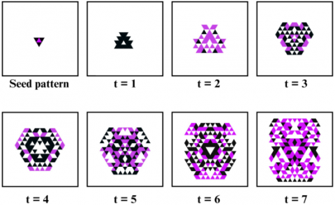
Figure 7. Application of rule r(vi,j) for the seed pattern 1 at time step 't = 1, 2, ...7'
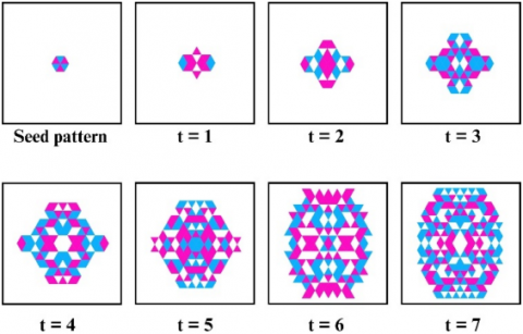
Figure 8. Application of rule r(vi,j) for the seed pattern 2 at time step 't = 1, 2, ...7'
Figures 7 and 8 depict the patterns evolved by applying the rule $r\left(v_{i, j}\right)$ for the seed pattern 1-2. The generations of seed pattern 1 is vertically symmetric and the generations of seed pattern 2 is both horizontally and vertically symmetric. The symmetric property is preserved through all the iterations or time steps by applying the rule $r\left(v_{i, j}\right)$. By applying Algorithm 1, the triangular lattice CA with 20 rows and 21 columns is updated with the states in the consecutive pattern evolutions. For each generation of the triangular lattice CA , the states 0,1 and 2 are coloured with three different colours such as, for seed pattern 1 - white, black, purple; for seed pattern 2 - white, pink, blue respectively.
A variety of patterns that cannot be generated by square lattice CA are observed to emerge in triangular lattices, often exhibiting extreme symmetry and well-organized structures. Unlike the square lattice, where a uniform neighborhood is applied throughout, the triangular lattice alternates between two different types of neighborhood configurations based on cell position. Despite this alternating scheme, the evolution process still produces highly aesthetic and coherent patterns, highlighting the richness and expressive power of the triangular lattice structure.
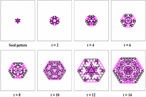
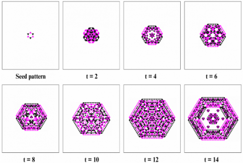
Figure 9. Application of rule r(vi,j) for the seed pattern 3 at time step 't = 0,2,4, ..., 14'
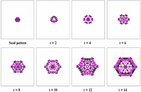
Figure 10. Application of rule r(vi,j) for the seed pattern 4 at time step 't = 0,2,4, ..., 14'
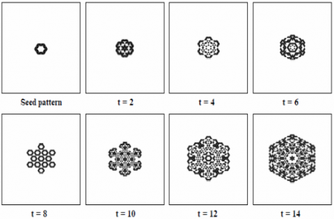
A set of figures are presented to illustrate the intricate structures produced by the algorithm. These figures display the emergence of hexagonal fractals and radially symmetric formations by their recursive growth. These patterns showcase its potential for creative applications in areas such as algorithmic art, digital textiles, and architectural tiling. Figures 9-11 depict the emergence of such aesthetic patterns from simple initial configurations. The patterns are generated using three distinct states, where white represents 0, black represents 1, and magenta represents 2. Figure 12 depicts the pattern generation with binary states. Square lattices possess only 4-fold rotational symmetry (90°), which restricts the formation of naturally radial or hexagonal patterns. Figures 9-11 exhibit 3-fold rotational symmetry and Figure 12 demonstrates a 6-fold rotational symmetry.
Figure 11. Application of rule r(vi,j) for the seed pattern 5 at time step 't = 0,2,4, ..., 14'
Figure 12. Application of rule r(vi,j) for the seed pattern 6 at time step 't = 0,2,4, ..., 14'
Transition rules are employed in computing the next configuration of the CA. Using a matrix allows for efficient application of transition rules across all cells simultaneously. The patterns evolved by applying the transition rule individually to each cell and the configurations obtained by applying the rule matrix method produce the same result for any finite $m \times n$ cellular automaton under any linear rule of the finite linear TLMCA.
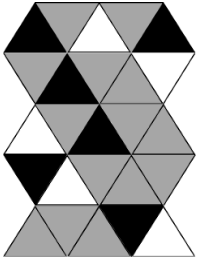
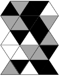
In particular, the Triangular Lattice Moore neighborhood CA has to deal with 13 neighborhood including itself. For instance, the configuration of a $5 \times 5$ TLMCA is taken here. The next configuration of current configuration is computed using both transition rule and transition rule matrices. Figure 13 depicts the lattice representing of states of the TLMCA. Black colour represents state 2, grey colour represents state 1 and white colour represents state 0.
Figure 13. Configuration at time ‘s’
5.1 Transition rule
Form the Figure 13, we have $\begin{aligned}v_{1,1}=v_{1,5}=v_{2,2}= v_{3,3}=v_{4,1}=v_{5,4}=2, v_{1,2}=v_{1,4}=v_{2,1}=v_{2,3}=v_{2,4}=v_{3,2}=v_{3,4}=v_{3,5}=v_{4,3}=v_{4,4}=v_{4,5}=1\text { and } v_{1,3}=v_{2,5}=v_{3,1}=v_{4,2}=v_{5,5}=0 .
\end{aligned}$
The values $\begin{aligned}a_0=d_0=0, a=b=c=a_1=a_2=a_3=b_1=b_2=b_3=c_1=c_2=c_3=d=e=f=d_1=d_2=d_3=e_1=e_2=e_3=f_1=f_2=f_3=1
\end{aligned}$
By applying the transition rule to each cell individually, we get
$r\left(v_{1,1}\right)=r\left(v_{1,3}\right)=r\left(v_{1,4}\right)=r\left(v_{2,3}\right)=r\left(v_{2,4}\right)$
$=r\left(\nu_{3,2}\right)=r\left(\nu_{3,4}\right)=r\left(\nu_{4,5}\right)=r\left(\nu_{5,2}\right)$
$=r\left(v_{5,4}\right)=r\left(v_{5,5}\right)=2, r\left(v_{1,2}\right)=r\left(v_{2,1}\right)$
$=r\left(v_{2,2}\right)=r\left(v_{2,5}\right)=r\left(v_{3,5}\right)=r\left(v_{4,3}\right)=r\left(v_{4,4}\right)$
$=r\left(v_{5,1}\right)=1$ and $r\left(v_{1,5}\right)=r\left(v_{3,1}\right)=r\left(v_{3,3}\right)$
$=r\left(v_{4,1}\right)=r\left(v_{4,2}\right)=r\left(v_{5,3}\right)=0$.
Therefore, the resulting next step configuration of the considered triangular lattice is depicted in Figure 14.
Figure 14. Configuration at time ‘s+1’
5.2 Rule matrix
The order of the considered CA is 5 × 5. Here m and n are odd positive integers. By proceeding with the methodology involved in theorem 1, the rule matrix is as follows of order 25 × 25.
$\mathcal{T}_{\mathcal{R}}^{55}=\left[\begin{array}{ccccc}\alpha_1 & \beta_1 & \mathcal{O} & \mathcal{O} & \mathcal{O} \\ \gamma_1 & \alpha_2 & \beta_2 & \mathcal{O} & \mathcal{O} \\ \mathcal{O} & \gamma_2 & \alpha_1 & \beta_1 & \mathcal{O} \\ \mathcal{O} & \mathcal{O} & \gamma_1 & \alpha_2 & \beta_2 \\ \mathcal{O} & \mathcal{O} & \mathcal{O} & \gamma_2 & \alpha_1\end{array}\right]$
where,
$\begin{array}{ll}\alpha_1=\left[\begin{array}{lllll}0 & 1 & 1 & 0 & 0 \\ 1 & 0 & 1 & 1 & 0 \\ 1 & 1 & 0 & 1 & 1 \\ 0 & 1 & 1 & 0 & 1 \\ 0 & 0 & 1 & 1 & 0\end{array}\right] & \alpha_2=\left[\begin{array}{lllll}0 & 1 & 1 & 0 & 0 \\ 1 & 0 & 1 & 1 & 0 \\ 1 & 1 & 0 & 1 & 1 \\ 0 & 1 & 1 & 0 & 1 \\ 0 & 0 & 1 & 1 & 0\end{array}\right] \\ \beta_1=\left[\begin{array}{lllll}1 & 1 & 1 & 0 & 0 \\ 1 & 1 & 1 & 0 & 0 \\ 1 & 1 & 1 & 1 & 1 \\ 0 & 0 & 1 & 1 & 1 \\ 0 & 0 & 1 & 1 & 1\end{array}\right] & \beta_2=\left[\begin{array}{lllll}1 & 1 & 0 & 0 & 0 \\ 1 & 1 & 1 & 1 & 0 \\ 0 & 1 & 1 & 1 & 0 \\ 0 & 1 & 1 & 1 & 1 \\ 0 & 0 & 0 & 1 & 1\end{array}\right]\end{array}$
$\gamma_1=\left[\begin{array}{lllll}1 & 1 & 1 & 0 & 0 \\ 1 & 1 & 1 & 0 & 0 \\ 1 & 1 & 1 & 1 & 1 \\ 0 & 0 & 1 & 1 & 1 \\ 0 & 0 & 1 & 1 & 1\end{array}\right] \quad \gamma_2=\left[\begin{array}{lllll}1 & 1 & 0 & 0 & 0 \\ 1 & 1 & 1 & 1 & 0 \\ 0 & 1 & 1 & 1 & 0 \\ 0 & 1 & 1 & 1 & 1 \\ 0 & 0 & 0 & 1 & 1\end{array}\right]$
$\left[T_R^{m n}\right] \cdot C^{\prime(s)}=C^{\prime(s+1)}$
We obtain a matrix which is the next step configuration of the given CA by applying rule matrix concept and is denoted by $C^{(s+1)}$
$C^{(s+1)}=\left[\begin{array}{lllll}2 & 1 & 2 & 2 & 0 \\ 1 & 1 & 2 & 2 & 1 \\ 0 & 2 & 0 & 2 & 1 \\ 0 & 0 & 1 & 1 & 2 \\ 1 & 2 & 0 & 2 & 2\end{array}\right]$
The configuration matrix $C^{(s+1)}$ exactly resembles the configuration obtained by applying the transition rule to all cells individually.
This study offers a comprehensive analysis of the algebraic structure and dynamic behavior of finite linear TLMCA under null boundary conditions. The Moore neighborhood for a triangular lattice is very complex, involving 13 neighbors. The local complexity influences the global complexity. The very common types of lattices involved in Cellular Automata are the square, triangular, and hexagonal lattices. This work decodes the logic behind the complex Moore triangular lattice Cellular Automata. By constructing rule matrices for the triangular lattice geometry and proposing an algorithm for their evolution, we have shown that such systems can generate distinct and complex patterns that are not possible with traditional square lattice Cellular Automata. The incorporation of a backward-tracing mechanism enables the exploration of reversible configurations, contributing to a more profound understanding of the conditions under which triangular lattice Cellular Automata exhibit reversibility. This has significant implications for applications such as cryptography, where reversibility and complexity are vital for secure key generation and encryption schemes. The proposed triangular lattice CA model successfully generates complex and structured patterns such as hexagonal fractals and radial symmetric motifs, characterized by recursive growth. The aesthetic coherence and geometric regularity of these patterns align with fundamental design principles, offering promising applications in fields such as algorithmic art, digital textile design, and architectural tiling. In the future, we will explore the integration of fuzzy logic or probabilistic transitions into this framework, expanding its applicability to uncertain or noisy environments. The analytical tools developed in this work also pave the way for classifying triangular CA rules based on complexity, reversibility, and computational universality.
[1] Neumann, J.V., Burks, A.W. (1966). Theory of self-reproducing automata. The Quarterly Review of Biology, 42(4): 521-523. https://doi.org/10.1086/405504
[2] Imai, K., Morita, K. (2000). A computation-universal two-dimensional 8-state triangular reversible cellular automaton. Theoretical Computer Science, 231(2): 181-191. https://doi.org/10.1016/S0304-3975(99)00099-7
[3] Morita, K., Margenstern, M., Imai, K. (1999). Universality of reversible hexagonal Cellular Automata. RAIRO-Theoretical informatics and Applications, 33(6): 535-550. https://doi.org/10.1051/ita:1999131
[4] Akin, H., Siap, I., Uğuz, S. (2010). Structure and Reversibility of 2-dimensional Hexagonal Cellular Automata. AIP Conference Proceedings, 1309(1): 16-26. https://doi.org/10.1063/1.3525111
[5] Bays, C. (2009). Cellular Automata in Triangular, Pentagonal, and Hexagonal Tessellations. In: Adamatzky, A. (eds) Cellular Automata. Encyclopedia of Complexity and Systems Science Series. Springer, New York, NY. https://doi.org/10.1007/978-0-387-30440-3_58
[6] Zawidzki, M. (2011). Application of Semitotalistic 2D Cellular Automata on a triangulated 3D surface. International Journal of Design & Nature and Ecodynamics, 6(1): 34-51. https://doi.org/10.2495/DNE-V6-N1-34-51
[7] Saadat, M., Nagy, B. (2018). Cellular Automata approach to mathematical morphology in the triangular grid. Acta Polytechnica Hungarica, 15(6): 45-62.
[8] Saadat, M.R., Nagy, B. (2021). Generating patterns on the triangular grid by Cellular Automata including alternating use of two rules. In 2021 12th International Symposium on Image and Signal Processing and Analysis (ISPA), Zagreb, Croatia, pp. 253-258. https://doi.org/10.1109/ISPA52656.2021.9552107
[9] Morita, K. (2016). Universality of 8-State Reversible and Conservative Triangular Partitioned Cellular Automata. In: El Yacoubi, S., Wąs, J., Bandini, S. (eds) Cellular Automata. ACRI 2016. Lecture Notes in Computer Science, vol. 9863. Springer, Cham. https://doi.org/10.1007/978-3-319-44365-2_5
[10] Moore, E.F. (1962). Machine models of self-reproduction. Proceedings of Symposia in Applied Mathematics, 14(5): 17-33.
[11] Das, A.K., Ganguly, A., Dasgupta, A., Bhawmik, S., Chaudhuri, P.P. (1990). Efficient characterisation of Cellular Automata. IEE Proceedings E (Computers and Digital Techniques), 137(1): 81-87. https://doi.org/10.1049/ip-e.1990.0008
[12] Das, A.K., Sanyal, A., Palchaudhuri, P. (1992). On characterization of Cellular Automata with matrix algebra. Information Sciences, 61(3): 251-277. https://doi.org/10.1016/0020-0255(92)90053-B
[13] Ganguly, N., Sikdar, B.K., Chaudhuri, P.P. (2008). Exploring cycle structures of additive Cellular Automata. Fundamenta Informaticae, 87(2): 137-154. https://doi.org/10.3233/FUN-2008-87202
[14] Pal Chaudhuri, P., Roy Chowdhury, D., Nandi, S., Chatterjee, S. (1997). Additive Cellular Automata–Theory and Applications. IEEE, Computer Society.
[15] Kaspar, A.J., Christy, D.S., Masilamani, V., Thomas, D.G. (2024). Two dimensional fuzzy context-free languages and tiling patterns. Fuzzy Sets and Systems, 485: 108961. https://doi.org/10.1016/j.fss.2024.108961
[16] Packard, N.H., Wolfram, S. (1985). Two-dimensional Cellular Automata. Journal of Statistical Physics, 38(5): 901-946. https://doi.org/10.1007/BF01010423
[17] Terrier, V. (2004). Two-dimensional Cellular Automata and their neighborhoods. Theoretical Computer Science, 312(2-3): 203-222. https://doi.org/10.1016/j.tcs.2003.08.011
[18] Durand, B. (1993). Global properties of 2D Cellular Automata: some complexity results. In: Borzyszkowski, A.M., Sokołowski, S. (eds) Mathematical Foundations of Computer Science 1993. MFCS 1993. Lecture Notes in Computer Science, vol 711. Springer, Berlin, Heidelberg. https://doi.org/10.1007/3-540-57182-5_35
[19] de Oliveira, G.M.B., Siqueira, S.R.C. (2006). Parameter characterization of two-dimensional Cellular Automata rule space. Physica D: Nonlinear Phenomena, 217(1): 1-6. https://doi.org/10.1016/j.physd.2006.02.010
[20] Kari, J. (1990). Reversibility of 2D Cellular Automata is undecidable. Physica D: Nonlinear Phenomena, 45(1-3): 379-385. https://doi.org/10.1016/0167-2789(90)90195-U
[21] Khan, A.R., Choudhury, P.P., Dihidar, K., Mitra, S., Sarkar, P. (1997). VLSI architecture of a Cellular Automata machine. Computers & Mathematics with Applications, 33(5): 79-94. https://doi.org/10.1016/S0898-1221(97)00021-7
[22] Sahin, U., Uguz, S., Akin, H. (2015). The transition rules of 2D linear Cellular Automata over ternary field and self-replicating patterns. International Journal of Bifurcation and Chaos, 25(1): 1550011. https://doi.org/10.1142/S021812741550011X
[23] Siap, I., Akin, H., Uğuz, S. (2011). Structure and reversibility of 2D hexagonal Cellular Automata. Computers & Mathematics with Applications, 62(11): 4161-4169. https://doi.org/10.1016/j.camwa.2011.09.066
[24] Dihidar, K., Choudhury, P.P. (2004). Matrix algebraic formulae concerning some exceptional rules of two-dimensional Cellular Automata. Information Sciences, 165(1-2): 91-101. https://doi.org/10.1016/j.ins.2003.09.024
[25] Zhai, Y., Yi, Z., Deng, P.M. (2009). On behavior of two-dimensional Cellular Automata with an exceptional rule. Information Sciences, 179(5): 613-622. https://doi.org/10.1016/j.ins.2008.10.024
[26] Chowdhury, D.R., Subbarao, P., Chaudhuri, P.P. (1993). Characterization of two-dimensional Cellular Automata using matrix algebra. Information sciences, 71(3): 289-314. https://doi.org/10.1016/0020-0255(93)90060-Y
[27] LuValle, B.J. (2019). The effects of boundary conditions on Cellular Automata. Complex Systems, 28(1): 97-124. https://doi.org/10.25088/ComplexSystems.28.1.97
[28] Sahin, U., Uguz, S., Akın, H., Siap, I. (2015). Three-state von Neumann Cellular Automata and pattern generation. Applied Mathematical Modelling, 39(7): 2003-2024. https://doi.org/10.1016/j.apm.2014.10.025
[29] Uguz, S., Redjepov, S., Acar, E., Akin, H. (2017). Structure and reversibility of 2D von Neumann Cellular Automata over triangular lattice. International Journal of Bifurcation and Chaos, 27(6): 1750083. https://doi.org/10.1142/S0218127417500833
[30] Ray, A., Laflamme, R., Kubica, A. (2024). Protecting information via probabilistic Cellular Automata. Physical Review E, 109(4): 044141. https://doi.org/10.1103/PhysRevE.109.044141
[31] Verhodubs, O. (2025). Application of ontology and cellular automaton to simulate the process of thought generation. SSRN. http://doi.org/10.2139/ssrn.5138819
[32] Kari, J. (2009). Lecture Notes on Cellular Automata. University of Turku.
[33] Bhattacharjee, K., Naskar, N., Roy, S., Das, S. (2020). A survey of Cellular Automata: types, dynamics, non-uniformity and applications. Natural Computing, 19: 433-461. https://doi.org/10.1007/s11047-018-9696-8