La'aly A. Al-Samrraie*![]() | Ayman M. Abdalla
| Ayman M. Abdalla![]() | Khalideh Al-Bkoor Alrawashdeh
| Khalideh Al-Bkoor Alrawashdeh![]() | Abeer Al Bsoul
| Abeer Al Bsoul![]() | Mohammad Abu Awad
| Mohammad Abu Awad![]() | Kamel Alzboon
| Kamel Alzboon![]() | Ahmed A. Al-Taani
| Ahmed A. Al-Taani![]()
© 2025 The authors. This article is published by IIETA and is licensed under the CC BY 4.0 license (http://creativecommons.org/licenses/by/4.0/).
OPEN ACCESS
This study is the first to compare deep learning models for rainfall prediction across several Jordanian cities representing diverse climates using 11 years of recorded climate data, something that previous studies have not addressed in the Jordanian context. The climate records for four Jordanian cities (Amman, Irbid, Karak, and Ajloun) were recorded hourly. The data was divided into training sets (80%) and test sets (20%), with and without the application of correlation analysis, feature selection, and data standardization steps applied. Three neural network models, Recurrent Neural Network (RNN), Long Short-Term Memory (LSTM), and Convolutional Neural Network-Recurrent Neural Network (CNN-RNN) were used to evaluate the performance of rainfall prediction in the four cities using three sets of features: all variables (13 features), precipitation only, and a selection of eight correlated features. The results showed that the RNN model outperformed the others overall, especially when using correlated features, recording the lowest error values, Mean Squared Error (MSE) and Root Mean Squared Error (RMSE) in most cities, with the exception of Amman, where the model performed best when using all features. Whereas in Irbid, the MSE was 0.0802×10⁻3 and RMSE = 0.009, while in Karak, the MSE was 0.118×10⁻3 and RMSE = 0.0109. In Amman, the RNN using all features achieved MSE = 0.0167×10⁻3 and RMSE = 0.0041.
Long Short-Term Memory (LSTM), deep learning, Convolutional Neural Network-Recurrent Neural Network (CNN-RNN), Recurrent Neural Network (RNN), weather forecast
In recent years, deep learning methodologies, particularly neural networks (NNs), have emerged as powerful tools for modeling complex nonlinear systems across various domains, including weather forecasting, water demand prediction, image recognition, computer vision, bioinformatics, and natural language processing [1-5]. Rainfall forecasting, a critical aspect of weather prediction, plays a pivotal role in water resource management and disaster mitigation strategies [6], due to prevailing arid conditions and the impact of climate change [7] For example, the Jordan Meteorological Department reported a national average of 88.95 millimeters (mm) of rainfall in 2021, compared to 144.99 mm in 2020 [8]. Historical data reveals even wider variations, with an average annual precipitation of 118.07 mm between 1901 and 2021, and extreme lows of 44.75 mm and 53.07 mm in 1944 and 2017, respectively.
Understanding the complex mechanisms behind precipitation, influenced by climatological and geographical factors, is essential for improving rainfall prediction accuracy, particularly in a geographically diverse country like Jordan. Jordan is divided into distinct rainfall zones, with annual precipitation levels ranging from less than 100 mm to over 300 mm [9]. About 80% of the country receives less than 100 mm of rainfall annually, while less than 5% receives over 300 mm. The northwestern upland areas experience the highest rainfall, ranging from 400 to 650 mm annually, whereas regions such as the northern Jordan Valley receive 200–250 mm, and the southern uplands receive less than 170 mm [10, 11].
Average annual rainfall in Jordan is low, at only about 118 mm, reflecting water scarcity and significant challenges in water resource management [8]. Under these challenging climatic conditions, accurate rainfall forecasting becomes vital to enhance drought mitigation strategies and improve dam management and water storage [12]. Recent studies in the Jordan Valley and the Middle East region in general have demonstrated the effectiveness of using deep learning models, such as LSTM and neural networks, in predicting rainfall with high accuracy, contributing to enhanced resilience to weather variability and improved water planning [13]. Other research has demonstrated the ability of these models to adapt to unusual climatic phenomena, increasing the reliability of forecasts in arid and semi-arid environments [14].
Previous studies have highlighted the potential of deep learning and neural networks in weather and rainfall forecasting. Early NN models demonstrated that larger datasets and deeper networks can reduce prediction errors [15]. Feature-based approaches, such as the one in reference [16], further enhanced the efficacy of deep learning models in weather studies.
Various neural network architectures have been employed for weather forecasting. For instance, Convolutional Neural Networks (CNNs) have been used to predict severe convective weather, such as thunderstorms and hail [17]. Hernández et al. [18] introduced a deep-learning approach using NNs and autoencoders for predicting rainfall accumulation, surpassing previous methods based on multiple metrics. However, their model was limited to a single city in Colombia and made only next-day predictions. In contrast, a deep-learning NN was developed for monthly rainfall forecasting in Thailand [19]. Additionally, in southern Taiwan, deep learning was applied for hourly rainfall prediction, showing that rainfall, pressure, and humidity significantly influenced prediction performance [20]. Aksoy and Dahamsheh [21] used neural networks to predict monthly rainfall in Jordan, while Freiwan and Cigizoglu [22] applied MLP to predict precipitation in semi-arid regions within Jordan. In 2024, Abuhammad et al [12] presented an LSTM model using data from the Jordanian Ministry of Water and Irrigation, achieving good performance in terms of RMSE and R². Subsequently, Tarawneh et al. [23] developed a hybrid CNN- Long Short-Term Memory model using daily Jordanian data, outperforming conventional models in its accuracy metrics. The inclusion of these studies reinforces the local and climatic background relevant to Jordan, providing a strong justification for the choice of deep learning models in the current context.
Recurrent Neural Networks (RNNs), a superset of feedforward NNs, are well-suited for processing sequential data, making them particularly effective for time-series analysis tasks such as weather prediction [24, 25]. RNNs are especially useful for providing timely and accurate weather predictions based on historical data [26].
Long Short-Term Memory (LSTM), a modern RNN architecture, contains memory cells that can store, read, and write data through the use of gates. LSTM networks have been applied to various sequential data tasks, such as text and motion capture prediction [27]. LSTM can be trained for sequence generation by processing and predicting real data sequences one step at a time [3, 28]. In hydrological modeling and rainfall-runoff simulation, LSTM networks have also been effective [27, 29], and comparative studies have demonstrated the efficacy of LSTM in time-series forecasting for rainfall prediction [24].
The CNN-RNN framework combines the strengths of CNNs and RNNs, making it a powerful tool for complex systems [4, 24, 30]. In recent years, researchers have begun expanding the use of CNNs to include non-traditional applications beyond image and map processing. They have been successfully employed in meteorological data analysis, given their ability to capture complex spatial patterns within rainfall data when represented on a grid or with numerical spatial distributions. This type of data, although temporal, is often affected by location-related geographic features, enabling CNN models to extract influential features that traditional RNNs cannot detect alone. By combining CNNs with LSTM or Gated Recurrent Unit, it becomes possible to create hybrid models capable of handling both temporal and spatial variations. Several recent studies have demonstrated a significant improvement in forecasting accuracy using this approach, especially in arid and semi-arid regions such as Jordan [31]. Therefore, the inclusion of CNN in this research model is scientifically justified and is expected to enhance the efficiency of rainfall forecasting in light of the large variation in the geographical distribution of rainfall in the Kingdom. For instance, Khaki et al. [30] used a CNN-RNN model to predict crop yield based on environmental data and management practices [32], and similar techniques can be adapted for weather forecasting, where temporal patterns and environmental factors are critical. Other combinations of deep learning techniques have also shown promise in improving weather prediction [33]. A literature review of deep learning techniques in weather forecasting is available in reference [1].
Abnormal climatic events such as droughts and excessive rains have had peculiar challenges with rainfall forecasting, with model performance varying based on factors such as the size of the dataset, the occurrence of extreme events in training data, and model flexibility. Though training on datasets with uncommon events can enhance the predictive accuracy by enabling models to learn prominent patterns, their lack can render performance under uncommon events invalid. Yet it has been found that deep learning models, especially LSTM, can make reasonably accurate forecasts even when operating under atypical conditions, reflecting some robustness even if these outliers are sub representations in training data [34]. Despite the advanced features of the LSTM model, such as its ability to handle long-term temporal dependencies and its relative resistance to outliers, its performance in this study lagged behind that of the RNN model in most cities. This is likely due to the nature of the temporal precipitation data used, as the data was hourly, meaning that the long-term dependencies that the LSTM leverages may be less salient or insufficient to enhance its performance. Furthermore, the LSTM requires a more complex training structure and fine-tuning of hyperparameters, making it more susceptible to performance degradation when data are insufficient or there is significant variability between cities. In contrast, the RNN model demonstrates superior performance at capturing short- and medium-term dependencies, which is consistent with the characteristics of the precipitation data in this study, explaining its comparatively superior results.
This study embarks on a comprehensive investigation into the predictive capabilities of different NN architectures using weather data from various cities in Jordan. Given that LSTM, RNN, and CNN-RNN have proven effective in weather prediction [26-29, 32, 35], this research aims to identify the most effective methods for rainfall prediction across Jordan's diverse regions. The four cities considered are Irbid in the northwest, Ajloun in the northern uplands, Amman in the central region, and Karak in the southern uplands. By focusing on cities representing diverse climatic zones, this study seeks to optimize rainfall forecasting models tailored to Jordan’s unique geographical and climatic conditions. The evaluation and comparison of these neural network architectures using robust metrics aim to determine the most accurate and reliable approaches for rainfall prediction, contributing to improved water resource management in Jordan. The results will be compared to identify the most effective neural network and feature selection method for forecasting rainfall in these cities.
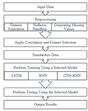
This paper presents a system for rainfall prediction using deep learning by implementing different (NN) models on real-world data. Figure 1 provides an overview of the methodology of the proposed system, with details explained in the following subsections. The selected NNs—LSTM, RNN, and CNN-RNN—were chosen based on their successful application in previous works [2, 26-28, 32, 35]. This study trains and tests these models, then evaluates and compares the results to determine the best model for rainfall prediction.
Figure 1. Diagram of the methodology of the proposed system
2.1 Dataset preprocessing
The dataset used in this study was obtained from the Open Weather website [36], comprising 13 weather features recorded for four cities in Jordan. These cities vary in elevation but are not coastal. The training data was collected hourly over 11 years.
The preprocessing steps prepare the dataset as follows:
For non-rainfall features with missing values (e.g., due to equipment errors), estimate the missing values using a linear function.
These preprocessing yields four distinct datasets, one for each city, with 13 features per city. These features are used as predictor variables, identified as covariates in the model and detailed further in the following section. The predictor variables influencing rainfall forecasting are listed in Table 1.
Missing data were handled through two imputation strategies. Rainfall values were imputed with zeros under the assumption that missing entries typically indicate no precipitation—a reasonable assumption for Jordan’s predominantly dry climate. While this simplifies data preparation, it may introduce bias if rainfall occurred during unrecorded intervals due to sensor failure, potentially affecting model accuracy. For the remaining meteorological variables, linear interpolation was used to estimate missing values by drawing a straight line between known data points. This method is appropriate when values change gradually over time, though it may fail to capture abrupt or nonlinear shifts inherent in meteorological phenomena.
Table 1. Weather features used as predictors
|
No. |
Name |
Description |
|
1 |
airT2 |
Air temperature at 2 meters |
|
2 |
ALLSKY KT |
All sky insolation clearness index |
|
3 |
ALLSKY SFC SW DWN |
Total solar irradiance incident |
|
4 |
CLRSKY SFC SW DWN |
Clear sky shortwave downward irradiance |
|
5 |
PS |
Surface pressure |
|
6 |
QV2M |
Humidity at 2 meters |
|
7 |
Rain |
Precipitation |
|
8 |
RH2M |
Relative humidity at 2 meters |
|
9 |
T2MDEW |
Dew/frost temperature at 2 meters |
|
10 |
T2MWET |
Wet bulb temperature at 2 meters |
2.2 Correlation and feature selection
To minimize redundant features in each city, a correlation matrix is computed for each parameter. Once the correlation matrix is calculated, only one instance of each redundant feature is retained for the subsequent steps, while other redundant features are removed.
2.3 Standardization
The dataset is standardized using the mean and standard deviation to avoid disturbances or spikes that could negatively impact training performance. The standardized value (z) of each reading (x) is calculated using Eq. (1), where μ is the mean and σ is the standard deviation.
$z=\frac{x-\mu}{\sigma}$ (1)
2.4 The implemented NN models
The application of LSTM, RNN, and CNN-RNN models shows promise for advancing rainfall prediction. LSTM models, with memory cells that retain information over extended periods, excel at capturing long-term dependencies within time-series data, making them ideal for modeling complex temporal patterns in rainfall behavior. RNN models, with recurrent connections, allow previous data points in the sequence to be considered, enhancing the network’s ability to discern sequential dependencies critical for accurate rainfall prediction. Additionally, CNN-RNN models combine the spatial analysis capabilities of CNNs with the sequential memory of RNNs, providing a comprehensive approach that effectively captures both spatial and temporal features in rainfall datasets. This model intelligently integrates two key dimensions of precipitation data: spatial and temporal. CNN layers first analyze the input data to extract fine-grained spatial features, such as the distribution of rainfall across the map and the detection of rain clusters in specific areas. This information is then fed to RNN or LSTM layers, which track how these patterns evolve over time and learn their sequence and periodic or abrupt behavior. This systematic sequence allows the model to gain a broader view and a deeper understanding of the interactions of space and time, increasing its forecasting efficiency and accuracy in dealing with the dynamics of rainfall phenomena. These diverse NN architectures contribute to a more robust understanding of the complex dynamics influencing rainfall forecasting and ultimately enhance the precision of rainfall prediction models.
2.5 Training and testing
Each dataset, corresponding to a different city, is trained and tested separately. The data is split into 80% for training and 20% for testing. Additionally, training and testing are conducted for each of the three NNs (LSTM, RNN, and CNN-RNN) independently. Finally, the results are evaluated and compared using various metrics to determine the most effective model for rainfall prediction.
2.6 Evaluation metrics
Table 2 shows the hyperparameters used to train the various models (RNN, LSTM, and CNN-RNN) on the dataset. The Adam-type optimization algorithm was used due to its high adaptive gradient capability, and the binary crossentropy loss function was adopted due to its suitability for binary classification tasks.
The data was split 80% for training and 20% for testing, with a batch size of 64 and a maximum number of epochs of 200. To fine-tune the model's hyperparameters, a validation split was used, using 20% of the training data to reduce the possibility of overfitting. This method is widely used in similar research, such as the study [37] on text classification using LSTMs and the study [38] on the use of Convolutional Neural Networks (CNNs) for natural language processing. The internal architecture of the models was optimized based on their performance on the validation set, with three hidden layers for simple shapes (RNN, CNN-RNN) and four layers for LSTM networks, with different gradations in the number of neurons.
Table 2. Initialization and optimization parameters of the neural network models used in the study
|
Parameter/ Hyperparameter |
Value |
Parameter/ Hyperparameter |
Value |
|
Training set % |
80 |
Maximum number of training epoch |
200 |
|
Testing set % |
20 |
Minimum batch size |
64 |
|
Optimize learning |
Adam |
No. of hidden layers |
4(100,100,75,75) For LSTM 3 (128,64,32) for RNN and CNN-RNNN |
The metrics used to evaluate the implementation results are described in Eqs. (2)-(5), where Measured represents a vector of actual parameter values and Computed represents a vector of the parameter values predicted by the NN. Since these metrics represent prediction error, lower values indicate better prediction performance.
Error$(\mathrm{i})=$ Measured$(\mathrm{i})-$ Computed$(\mathrm{i})$ (2)
Mean Squared Error: $M S E=\frac{1}{n} \sum_{i=1}^n\left(\operatorname{Error}(i)^2\right)$ (3)
Root Mean Square Error: $R M S E=\sqrt{M S E}$ (4)
Normalized Root Mean Square Error: $\text { NRMSE }=\frac{\text { RMSE }}{\sum_{i=1}^n(\text {Computed }(i))}$ (5)
The data used in this study were obtained from the Open Weather website [36], consisting of hourly records over 11 years for four Jordanian cities: Amman, Irbid, Ajloun, and Karak. These were prearranged into four separate datasets, corresponding to the four cities, with each dataset partitioned into 80% for training and 20% for testing. All models—RNN, CNN-RNN, and LSTM—were trained using a batch size of 64 over a maximum of 200 epochs. The RNN architecture comprised four hidden layers with memory cell sizes of 128, 64, and 32, while the LSTM model included two hidden layers with memory units of sizes 64 and 32. The CNN-RNN hybrid integrated convolutional and recurrent layers across eight hidden layers, also employing memory cells of sizes 128, 64, and 32. All models were optimized using the Adam algorithm and operated in a unidirectional mode (i.e., without backward processing).
Correlation analysis, feature selection, and standardization were applied to each dataset as outlined in the Methodology section. The correlation matrices for the four datasets are shown in Tables 3-6. While there are limited differences among the correlation matrices, some features appeared independent, while others were redundant. As a result, only eight features were used for further analysis, including six features listed in Table 1: QV2M, PS, WS10M, Rain, airT2, and CLRSKY SFC SW DWN-along with two combined features: T2M (Temperature at 2 Meters) and PRECTOTCORR (Corrected Precipitation).
Table 3. Correlation matrix for Amman
|
Rain |
QV2M |
airT2 |
WS10M |
CLRSKY SFC SW DWN |
ALLSKY SFC SW DWN |
T2MWET |
PS |
ALLSKY KT |
RH2M |
T2MDEW |
WD50M |
WS50M |
|
1 |
-0.023 |
-0.153 |
0.205 |
-0.016 |
-0.057 |
-0.116 |
-0.091 |
-0.003 |
0.164 |
-0.003 |
0.008 |
0.193 |
|
-0.023 |
1 |
0.249 |
-0.149 |
-0.213 |
-0.2 |
0.665 |
-0.462 |
-0.201 |
0.419 |
0.971 |
0.463 |
-0.144 |
|
-0.153 |
0.249 |
1 |
0.128 |
0.578 |
0.61 |
0.881 |
-0.536 |
0.465 |
-0.717 |
0.27 |
0.299 |
-0.094 |
|
0.205 |
-0.149 |
0.128 |
1 |
0.271 |
0.232 |
0.021 |
-0.159 |
0.273 |
-0.248 |
-0.152 |
0.018 |
0.903 |
|
-0.016 |
-0.213 |
0.578 |
0.271 |
1 |
0.986 |
0.342 |
-0.132 |
0.738 |
-0.633 |
-0.183 |
0.062 |
-0.063 |
|
-0.057 |
-0.2 |
0.61 |
0.232 |
0.986 |
1 |
0.371 |
-0.134 |
0.72 |
-0.649 |
-0.173 |
0.062 |
-0.098 |
|
-0.116 |
0.665 |
0.881 |
0.021 |
0.342 |
0.371 |
1 |
-0.636 |
0.262 |
-0.329 |
0.694 |
0.46 |
-0.148 |
|
-0.091 |
-0.462 |
-0.536 |
-0.159 |
-0.132 |
-0.134 |
-0.636 |
1 |
-0.092 |
0.147 |
-0.477 |
-0.389 |
-0.082 |
|
-0.003 |
-0.201 |
0.465 |
0.273 |
0.738 |
0.72 |
0.262 |
-0.092 |
1 |
-0.555 |
-0.174 |
0.025 |
-0.037 |
|
0.164 |
0.419 |
-0.717 |
-0.248 |
-0.633 |
-0.649 |
-0.329 |
0.147 |
-0.555 |
1 |
0.419 |
0.083 |
-0.06 |
|
-0.003 |
0.971 |
0.27 |
-0.152 |
-0.183 |
-0.173 |
0.694 |
-0.477 |
-0.174 |
0.419 |
1 |
0.482 |
-0.157 |
|
0.008 |
0.463 |
0.299 |
0.018 |
0.062 |
0.062 |
0.46 |
-0.389 |
0.025 |
0.083 |
0.482 |
1 |
-0.048 |
|
0.193 |
-0.144 |
-0.094 |
0.903 |
-0.063 |
-0.098 |
-0.148 |
-0.082 |
-0.037 |
-0.06 |
-0.157 |
-0.048 |
1 |
Table 4. Correlation matrix for Irbid
|
Rain |
QV2M |
airT2 |
WS10M |
CLRSKY SFC SW DWN |
ALLSKY SFC SW DWN |
T2MWET |
PS |
ALLSKY KT |
RH2M |
T2MDEW |
WD50M |
WS50M |
|
1 |
-0.054 |
-0.143 |
0.125 |
-0.012 |
-0.063 |
-0.121 |
-0.036 |
0.001 |
0.126 |
-0.034 |
0.03 |
0.164 |
|
-0.054 |
1 |
0.295 |
-0.259 |
-0.211 |
-0.197 |
0.691 |
-0.549 |
-0.184 |
0.377 |
0.974 |
0.373 |
-0.3 |
|
-0.143 |
0.295 |
1 |
0.312 |
0.654 |
0.688 |
0.887 |
-0.615 |
0.525 |
-0.73 |
0.309 |
0.374 |
0.014 |
|
0.125 |
-0.259 |
0.312 |
1 |
0.344 |
0.314 |
0.116 |
-0.199 |
0.346 |
-0.485 |
-0.235 |
0.142 |
0.874 |
|
-0.012 |
-0.211 |
0.654 |
0.344 |
1 |
0.982 |
0.392 |
-0.175 |
0.737 |
-0.743 |
-0.185 |
0.154 |
0.031 |
|
-0.063 |
-0.197 |
0.688 |
0.314 |
0.982 |
1 |
0.423 |
-0.185 |
0.714 |
-0.757 |
-0.174 |
0.151 |
0 |
|
-0.121 |
0.691 |
0.887 |
0.116 |
0.392 |
0.423 |
1 |
-0.723 |
0.31 |
-0.355 |
0.713 |
0.47 |
-0.129 |
|
-0.036 |
-0.549 |
-0.615 |
-0.199 |
-0.175 |
-0.185 |
-0.723 |
1 |
-0.116 |
0.187 |
-0.556 |
-0.376 |
-0.082 |
|
0.001 |
-0.184 |
0.525 |
0.346 |
0.737 |
0.714 |
0.31 |
-0.116 |
1 |
-0.647 |
-0.159 |
0.111 |
0.067 |
|
0.126 |
0.377 |
-0.73 |
-0.485 |
-0.743 |
-0.757 |
-0.355 |
0.187 |
-0.647 |
1 |
0.375 |
-0.072 |
-0.242 |
|
-0.034 |
0.974 |
0.309 |
-0.235 |
-0.185 |
-0.174 |
0.713 |
-0.556 |
-0.159 |
0.375 |
1 |
0.4 |
-0.287 |
|
0.03 |
0.373 |
0.374 |
0.142 |
0.154 |
0.151 |
0.47 |
-0.376 |
0.111 |
-0.072 |
0.4 |
1 |
0.04 |
|
0.164 |
-0.3 |
0.014 |
0.874 |
0.031 |
0 |
-0.129 |
-0.082 |
0.067 |
-0.242 |
-0.287 |
0.04 |
1 |
Table 5. Correlation matrix for Ajloun
|
Rain |
QV2M |
airT2 |
WS10M |
CLRSKY SFC SW DWN |
ALLSKY SFC SW DWN |
T2MWET |
PS |
ALLSKY KT |
RH2M |
T2MDEW |
WD50M |
WS50M |
|
1 |
-0.054 |
-0.143 |
0.125 |
-0.012 |
-0.063 |
-0.121 |
-0.036 |
0.001 |
-0.034 |
0.126 |
0.164 |
0.03 |
|
-0.054 |
1 |
0.295 |
-0.259 |
-0.211 |
-0.197 |
0.691 |
-0.549 |
-0.184 |
0.974 |
0.377 |
-0.3 |
0.373 |
|
-0.143 |
0.295 |
1 |
0.312 |
0.654 |
0.688 |
0.887 |
-0.615 |
0.525 |
0.309 |
-0.73 |
0.014 |
0.374 |
|
0.125 |
-0.259 |
0.312 |
1 |
0.344 |
0.314 |
0.116 |
-0.199 |
0.346 |
-0.235 |
-0.485 |
0.874 |
0.142 |
|
-0.012 |
-0.211 |
0.654 |
0.344 |
1 |
0.982 |
0.392 |
-0.175 |
0.737 |
-0.185 |
-0.743 |
0.031 |
0.154 |
|
-0.063 |
-0.197 |
0.688 |
0.314 |
0.982 |
1 |
0.423 |
-0.185 |
0.714 |
-0.174 |
-0.757 |
0 |
0.151 |
|
-0.121 |
0.691 |
0.887 |
0.116 |
0.392 |
0.423 |
1 |
-0.723 |
0.31 |
0.713 |
-0.355 |
-0.129 |
0.47 |
|
-0.036 |
-0.549 |
-0.615 |
-0.199 |
-0.175 |
-0.185 |
-0.723 |
1 |
-0.116 |
-0.556 |
0.187 |
-0.082 |
-0.376 |
|
0.001 |
-0.184 |
0.525 |
0.346 |
0.737 |
0.714 |
0.31 |
-0.116 |
1 |
-0.159 |
-0.647 |
0.067 |
0.111 |
|
-0.034 |
0.974 |
0.309 |
-0.235 |
-0.185 |
-0.174 |
0.713 |
-0.556 |
-0.159 |
1 |
0.375 |
-0.287 |
0.4 |
|
0.126 |
0.377 |
-0.73 |
-0.485 |
-0.743 |
-0.757 |
-0.355 |
0.187 |
-0.647 |
0.375 |
1 |
-0.242 |
-0.072 |
|
0.164 |
-0.3 |
0.014 |
0.874 |
0.031 |
0 |
-0.129 |
-0.082 |
0.067 |
-0.287 |
-0.242 |
1 |
0.04 |
|
0.03 |
0.373 |
0.374 |
0.142 |
0.154 |
0.151 |
0.47 |
-0.376 |
0.111 |
0.4 |
-0.072 |
0.04 |
1 |
Table 6. Correlation matrix for Karak
|
Rain |
QV2M |
airT2 |
WS10M |
CLRSKY SFC SW DWN |
ALLSKY SFC SW DWN |
T2MWET |
PS |
ALLSKY KT |
RH2M |
T2MDEW |
WD50M |
WS50M |
|
1 |
-0.031 |
-0.146 |
0.14 |
-0.055 |
-0.025 |
-0.117 |
0.01 |
-0.015 |
-0.019 |
0.154 |
0.131 |
0.028 |
|
-0.031 |
1 |
0.265 |
-0.414 |
-0.168 |
-0.183 |
0.684 |
-0.413 |
-0.177 |
0.974 |
0.419 |
-0.422 |
0.155 |
|
-0.146 |
0.265 |
1 |
0.084 |
0.595 |
0.564 |
0.876 |
-0.623 |
0.46 |
0.279 |
-0.713 |
-0.101 |
0.35 |
|
0.14 |
-0.414 |
0.084 |
1 |
0.239 |
0.272 |
-0.149 |
-0.041 |
0.293 |
-0.419 |
-0.388 |
0.932 |
0.061 |
|
-0.055 |
-0.168 |
0.595 |
0.239 |
1 |
0.986 |
0.367 |
-0.168 |
0.72 |
-0.143 |
-0.626 |
-0.017 |
0.238 |
|
-0.025 |
-0.183 |
0.564 |
0.272 |
0.986 |
1 |
0.337 |
-0.154 |
0.738 |
-0.156 |
-0.611 |
0.012 |
0.243 |
|
-0.117 |
0.684 |
0.876 |
-0.149 |
0.367 |
0.337 |
1 |
-0.667 |
0.262 |
0.707 |
-0.315 |
-0.292 |
0.35 |
|
0.01 |
-0.413 |
-0.623 |
-0.041 |
-0.168 |
-0.154 |
-0.667 |
1 |
-0.117 |
-0.416 |
0.273 |
0.026 |
-0.272 |
|
-0.015 |
-0.177 |
0.46 |
0.293 |
0.72 |
0.738 |
0.262 |
-0.117 |
1 |
-0.151 |
-0.532 |
0.067 |
0.201 |
|
-0.019 |
0.974 |
0.279 |
-0.419 |
-0.143 |
-0.156 |
0.707 |
-0.416 |
-0.151 |
1 |
0.419 |
-0.434 |
0.184 |
|
0.154 |
0.419 |
-0.713 |
-0.388 |
-0.626 |
-0.611 |
-0.315 |
0.273 |
-0.532 |
0.419 |
1 |
-0.239 |
-0.189 |
|
0.131 |
-0.422 |
-0.101 |
0.932 |
-0.017 |
0.012 |
-0.292 |
0.026 |
0.067 |
-0.434 |
-0.239 |
1 |
-0.027 |
|
0.028 |
0.155 |
0.35 |
0.061 |
0.238 |
0.243 |
0.35 |
-0.272 |
0.201 |
0.184 |
-0.189 |
-0.027 |
1 |
Each of the three NNs (LSTM, RNN, and CNN-RNN) was trained and tested separately. Each model contained four hidden layers: the first two hidden layers had 100 units, while the third and fourth had 75 units. Training was conducted for 200 epochs, with 1,095 iterations per epoch.
To evaluate the impact of different parameters on rainfall prediction, the NNs were trained and tested in three separate trials: using all 13 features, using only the rainfall feature, and using the eight features selected through correlation and feature selection. The results of the performance assessment for different NNs and feature selection methods in forecasting rainfall in Amman, Irbid, Karak, and Ajloun are shown in Tables 7-10, respectively.
Table 7. Performance assessment of different NNs and feature selection methods in forecasting rainfall in Amman
|
Method |
Metrics with All Features |
Metrics with the Rainfall Feature |
Metrics with the Correlated Features |
||||||
|
MSE 10-3 |
RMSE 10-2 |
NRMSE |
MSE 10-3 |
RMSE 10-2 |
NRMSE |
MSE 10-3 |
RMSE 10-2 |
NRMSE |
|
|
LSTM |
2.9959 |
5.4734 |
2.3284 |
6.1611 |
7.8493 |
3.1736 |
1.740 |
4.1724 |
1.7749 |
|
CNN-RNN |
0.3071 |
1.75 |
0.7455 |
16.5 |
12.86 |
5.4721 |
0.5795 |
2.4 |
1.0241 |
|
RNN |
0.0167 |
0.41 |
0.1740 |
6.2 |
7.89 |
3.3551 |
0.0262 |
0.51 |
0.2178 |
Table 8. Performance assessment of different NNs and feature selection methods in forecasting rainfall in Irbid
|
Method |
Metrics with All Features |
Metrics with the Rainfall Feature |
Metrics with the Correlated Features |
||||||
|
MSE 10-3 |
RMSE 10-2 |
NRMSE |
MSE 10-3 |
RMSE 10-2 |
NRMSE |
MSE 10-3 |
RMSE 10-2 |
NRMSE |
|
|
LSTM |
6.1664 |
7.8527 |
1.7813 |
31.238 |
17.674 |
3.6027 |
5.811 |
7.6236 |
1.7293 |
|
CNN-RNN |
62.1 |
24.93 |
5.6543 |
63.0 |
25.11 |
5.6947 |
0.9699 |
3.0 |
0.7065 |
|
RNN |
0.0832 |
0.91 |
0.2069 |
25.23 |
15.88 |
3.6033 |
0.0518 |
0.72 |
0.1634 |
For period from 2018-2021, among the three NNs, RNN consistently produced the lowest error metrics for all cities. The other two NNs did not show a clear second-best performance. When using only the rainfall feature, RNN produced the lowest MSE and RMSE values for Amman (MSE = 0.0062, RMSE = 0.0789, and NMSE = 3.355), while LSTM performed best for Irbid (MSE = 0.0278, RMSE = 0.16943, and NMSE = 3.4536). Notably, LSTM also had the lowest NRMSE values across all cities. For the trial using only correlated features, RNN again produced the lowest error values for all cities, while CNN-RNN emerged as the second-best model.
To analyze the differences in prediction accuracy between the proposed models, the Diebold-Mariano (DM) test was used to measure whether the differences in performance between the models were statistically significant. The analysis was based on data from Table 7, which displays the results for the three models: the LSTM model, the CNN-RNN model, and the RNN model. The results showed that the RNN achieved the best performance overall and was therefore used as the reference model for comparison. When comparing the LSTM with RNN, the DM test revealed a statistically significant difference (p < 0.05), indicating that the performance of the LSTM is significantly less accurate than the RNN.
When comparing the LSTM with CNN-RNN, the results did not reveal a statistically significant difference between the two models, indicating that the performance of both models is similar in terms of prediction accuracy. Furthermore, the comparison between CNN-RNN and the RNN did not reveal any strong statistically significant differences. CNN-RNN did not clearly outperform RNN, but it was not significantly worse either. Based on the DM test values, it can be argued that the RNN model has relatively higher performance compared to the LSTM model, while it is not possible to assert that there are strong differences between the RNN model and the CNN-RNN model. The lack of significant differences between LSTM and CNN-RNN indicates a convergence in their prediction ability, although RNN still outperforms both.
The results of the DM test in Table 8 show that the RNN statistically outperforms the LSTM, reaching a significance level of (p = 0.007), which is less than 0.05, indicating that the difference in performance between the two models is clearly statistically significant in favor of RNN. In contrast, the comparison between the CNN-RNN and the RNN did not reveal any significant difference (p = 0.2777), and the comparison between the LSTM and the CNN-RNN did not yield any statistically significant differences either (p = 0.3686). Based on these results, it can be concluded that the RNN model performs better, with a significant superiority over LSTM. However, there are no strong statistical differences between RNN and CNN-RNN, nor between LSTM and CNN-RNN, indicating a convergence in their performance.
As shown in Table 9, there is no statistically significant difference between the third model (RNN) and both LSTM and CNN-RNN models. The p-values for both comparisons were greater than 0.05 (p = 0.0885 and p = 0.2885, respectively). Although the difference between RNN and LSTM was close to the significance level, it was not statistically significant. On the other hand, the comparison between LSTM and CNN-RNN showed a clear significant difference (p = 0.0025), indicating that LSTM performs significantly worse than CNN-RNN. Thus, it can be concluded that CNN-RNN is statistically superior to LSTM, while there are no confirmed significant differences between RNN and the other models, although the general trend suggests that RNN may perform better.
Table 9. Performance assessment of different NNs and feature selection methods in forecasting rainfall in Karak
|
Method |
Metrics with All Features |
Metrics with the Rainfall Feature |
Metrics with the Correlated Features |
||||||
|
MSE 10-3 |
RMSE 10-2 |
NRMSE |
MSE 10-3 |
RMSE 10-2 |
NRMSE |
MSE 10-3 |
RMSE 10-2 |
NRMSE |
|
|
LSTM |
14.144 |
11.893 |
2.6582 |
33.464 |
18.293 |
4.3038 |
14.52 |
12.05 |
2.6933 |
|
CNN-RNN |
1.5 |
3.92 |
0.8766 |
101.2 |
31.82 |
7.1106 |
1.8 |
4.29 |
0.9585 |
|
RNN |
0.0773 |
0.88 |
0.1965 |
67.82 |
26.0 |
5.820 |
0.1189 |
1.09 |
0.2437 |
Table 10. Performance assessment of different NNs and feature selection methods in forecasting rainfall in Ajloun
|
Method |
Metrics with All Features |
Metrics with the Rainfall Feature |
Metrics with the Correlated Features |
||||||
|
MSE 10-3 |
RMSE 10-2 |
NRMSE |
MSE 10-3 |
RMSE 10-2 |
NRMSE |
MSE 10-2 |
RMSE 10-2 |
NRMSE |
|
|
LSTM |
6.8339 |
8.2667 |
1.8752 |
28.707 |
16.943 |
3.4536 |
6.8339 |
8.2667 |
1.8752 |
|
CNN-RNN |
1.2 |
3.49 |
0.7918 |
62.5 |
25.00 |
5.6711 |
1.5 |
4.0 |
0.8910 |
|
RNN |
0.1087 |
1.04 |
0.2365 |
27.3 |
16.52 |
3.7483 |
0.0802 |
0.90 |
0.2032 |
Upon examining the results in Table 10, it is clear that RNN clearly demonstrates its superiority, especially when compared to LSTM. The DM test showed a strong statistical difference between the two models (p = 0.0008), clearly reflecting the superior performance of the RNN model. On the other hand, other comparisons appear less conclusive. The comparison between CNN-RNN and RNN did not show a clear statistical significance (p = 0.1210), indicating a convergence in performance without significant superiority. Similarly, the results did not show a significant difference between the LSTM and the CNN-RNN (p = 0.1323), although the overall trend favors the CNN-RNN.
Looking at the experimental results across the four Tables 7-10, RNN maintains consistently superior performance compared to the other two models, with clear statistical significance in several cases, especially compared to LSTM. This reinforces its credibility as a more efficient model in predictive accuracy. In contrast, CNN-RNN demonstrated comparable performance with RNN without consistent significant differences, making it a flexible choice in some scenarios. LSTM performed poorly in most comparisons, both in terms of values and statistical significance. In general, RNN can be considered a reliable reference model in situations requiring high accuracy supported by statistical analysis. CNN-RNN can be considered a potential alternative, while caution is recommended when relying on LSTM in applications that are sensitive to predictive performance.
In developing rainfall forecasting models tailored to Jordan, it was essential to account for the country’s varied climatic regions, which can significantly influence model training and predictive performance. Jordan encompasses multiple climate zones, including the Mediterranean-influenced northwestern region (e.g., Amman and Irbid), which receives between 245 mm and 450 mm of annual rainfall; the semi-arid Jordan Valley, with approximately 400 mm per year; and the arid eastern and southern regions, where annual rainfall often falls below 100 mm. This climatic variability refined the choice of characteristics that were introduced into the dataset. Topmost priority was given to parameters like temperature and humidity, which play important roles in precipitation processes in areas with moderate to high precipitation and varying temperatures. Attributes with little applicability in Jordan's climate, however, like snow, were eliminated because of the very low frequency of their occurrence. By correlating feature selection with the country's seasonal weather conditions, the study makes sure that the forecasting models are contextually relevant and will have a better opportunity to capture the rainfall patterns of Jordan.
Selecting the relevant meteorological factors is perhaps one of the most critical activities when developing accurate models for rainfall prediction because it immediately affects the efficacy of the models. For the purpose of this study, the main variables—temperature, humidity, wind speed, atmospheric pressure, and historic rainfall data—were collected from reputable meteorological sources throughout Jordan. Pearson correlation assessment was employed to identify correlations between these variables and rainfall so that those with moderate to strong relationships were included in the models and utilized. In addition to statistical validation, choice was also facilitated by findings of regional climatological studies and local weather expertise to validate that the features under consideration are data-driven as well as contextually relevant to Jordan's distinctive climate. Each of the variables chosen has a well-recognized function in the dynamics of precipitation: temperature influences atmospheric pressure and humidity; humidity indicates the moisture required for cloud development; wind speed controls air mass transport and weather front advancement; atmospheric pressure assists in determining low-pressure systems that precede rain; and historical rainfall data draw temporal patterns that are crucial to predictive model construction. This knowledge and systematic feature selection process increase the validity and situational relevance of the forecasting models established in this research.
Lower values of MSE, RMSE, and NRMSE (Tables 7-10) indicate better prediction results, as they reflect lower estimation errors. By examining the metrics (Tables 3-6) and the performance assessment (Tables 7-10), it becomes evident that the results from using only the rainfall feature were inferior to those obtained using either all features or the correlated features. Therefore, the comparison focuses on the latter two methods.
When analyzing the results produced by each NN, it is observed that LSTM and CNN-RNN performed better with all features than with correlated features across all cities. On the other hand, RNN produced the lowest MSE and RMSE values when using correlated features for Irbid (MSE = 8.0249×10⁻⁵, RMSE = 0.0090, and NMSE = 0.2032) and Karak (MSE = 1.1887×10⁻⁴, RMSE = 0.0109, and NMSE = 0.2437) (Table 4 and Table 6). For Amman, however, the lowest MSE and RMSE values were obtained by RNN using all features (MSE = 1.6733×10⁻⁵, RMSE = 0.0041, and NMSE = 0.1740) (Table 3).
Based on the data in Tables 7-10, the RNN model using correlated features was the most effective method for rainfall prediction in all cities except Amman, where the all-features method produced the most accurate results. Consequently, the combination of RNN with correlated features is considered the most appropriate approach for rainfall estimation. The results indicate that models using only the rainfall feature alone resulted in inferior predictive accuracy, showing higher error values than models utilizing either all features or a subset of correlated features. This suggests that rainfall predictions benefit from incorporating additional environmental variables, probably because rainfall is influenced by multiple but interconnected weather patterns. The topography of each city is a crucial factor in explaining the variation in model performance across different locations. For example, Irbid is located at a relatively lower elevation and is surrounded by open agricultural lands, making the influence of air masses and rainfall patterns more uniform and predictable. In contrast, Amman is characterized by a complex terrain ranging from hills to valleys, along with the presence of the urban heat island phenomenon resulting from dense urban sprawl. This impacts local airflow patterns and surface temperature, creating variations in rainfall distribution on small scales that are difficult for models to accurately capture. This topographical and climatic variation between cities directly affects the accuracy of models. Temporal models perform better in environments with uniform and open weather patterns, while they face challenges in cities with spatial and climatic complexity. By using all features or a focused subset of correlated features, the models capture a more comprehensive picture of the conditions affecting rainfall, thus improving forecast accuracy.
3.1 City-specific model performance and predictive insight
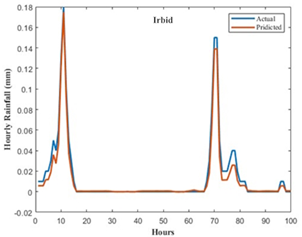
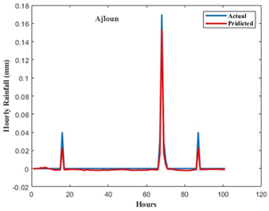
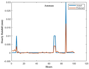
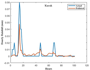
Figure 2 illustrates the actual rainfall data versus the predicted values by the RNN system for the four cities. The small differences between actual and predicted values demonstrate the efficacy of the RNN in making accurate rainfall predictions.
(a)
(b)
(c)
(d)
Figure 2. Actual vs. RNN predicted rainfall maps for Irbid, Ajloun, Amman and Karak
In Amman, the RNN model demonstrated the most consistent predictive accuracy across all configurations - utilizing the full set of features, the rainfall feature alone, and the selected correlated features (Figure 2). With the lowest MSE and RMSE values (Table 7), RNN proved especially effective in capturing Amman’s temporal rainfall patterns. LSTM models, while capable of capturing long-term dependencies, appeared slightly less adaptable in this city’s data context, probably due to the shorter temporal dependencies in Amman’s rainfall patterns. CNN-RNN, which combines spatial and sequential learning, was also effective but displayed relatively higher error metrics (Table 3), suggesting that spatial feature extraction may be less relevant in Amman’s meteorological data than temporal relationships. Based on this data, it can be said that rainfall in Jordan is close to zero in some areas in the south, while it is gradually increasing in the northern regions and highlands. However, the Kingdom continues to suffer from scarce water resources due to climate change and a general decline in rainfall rates [8, 39].
In the Irbid region, the model results showed that the RNN model performed best when using the full set of features, as shown in Table 8, clearly outperforming the LSTM and CNN-RNN models in terms of prediction accuracy. This superiority can be explained by the RNN's ability to capture the temporal relationships associated with rainfall patterns in the region, which are crucial for accurate forecasting. Although the CNN-RNN model has the ability to extract spatial features, this was not sufficient to surpass the effectiveness of the RNN in this case, indicating that temporal information plays a more important role in Irbid's climate, despite the presence of some spatial interactions. The LSTM model demonstrated acceptable performance, but it was unable to match the accuracy of the RNN, especially in representing the fine-scale variations in rainfall in Irbid.
In Karak, RNN models were consistently the most accurate, particularly with the correlated feature set (Figure 2 and Table 9). This performance highlights the importance of sequential dependencies in Karak’s rainfall prediction, where the model’s ability to consider prior time steps significantly enhanced forecast precision. LSTM models showed moderate performance, performing well on more complex configurations but still falling short of RNN accuracy. CNN-RNN models, while capable of incorporating spatial dependencies, did not outperform RNN, probably due to the relatively homogenous spatial distribution of weather patterns in Karak, which limited the utility of CNN-based spatial feature extraction. This finding suggests that in Karak, purely temporal relationships are more predictive of rainfall behavior than combined spatiotemporal patterns.
Ajloun’s model performance was unique in that RNN and CNN-RNN models performed comparably, each excelling in different configurations (Table 7 and Figure 2). The RNN model achieved the lowest error rates when using the correlated feature set, consistent with findings in other cities, underscoring RNN’s strength in time-series prediction. However, CNN-RNN demonstrated comparable accuracy when utilizing the complete set of features, suggesting that in Ajloun, a combination of spatial and temporal features captures underlying weather dynamics. LSTM models, while performing adequately, did not match the precision of RNN and CNN-RNN, indicating that the sequential dependency pattern in Ajloun is best captured by models emphasizing immediate past conditions rather than long-term memory.
Across the four cities, RNN models generally showed the highest accuracy, particularly with the reduced set of correlated features, highlighting their capacity to handle short-to-medium term temporal dependencies effectively. CNN-RNN models demonstrated added value in cities with more complex spatial dynamics, such as Irbid and Ajloun, where combined spatial-temporal patterns played a role in weather variability. Conversely, LSTM models, despite their strengths in capturing long-term dependencies, were generally less effective, indicating that rainfall in these urban regions may not require the extensive memory capabilities LSTM offers but rather benefits from models focused on recent sequential patterns.
In addition, by prediction hourly precipitation over a 100-hour period from 2018 to 2021, the RNN model demonstrated excellent forecast performance in most Jordanian cities. The highest rain average per hour was achieved in Amman, with an estimated of only 0.017 mm from the actual values, followed by Karak with a difference of 0.048 mm, Irbid with a difference of 0.18 mm, and finally Ajloun with a difference of 0.15 mm. When the rainfall prediction process was implemented for 100 random hours, the error rate between the actual and predicted values was found to be as follows: 43.33% in Amman, 40% in Karak, 1.11% in Irbid, and 11.76% in Ajloun. Based on these results, it is clear that Irbid recorded the lowest prediction error rate, indicating higher model accuracy there, while Amman had the highest error rate, which may reflect greater prediction challenges in its changing climate.
The results of this study are partially consistent with those at Najd Al `Azab, Yemen [40], which demonstrated that using correlated climate features can improve the accuracy of AI-based models in predicting rainfall in the Middle East, particularly in arid and semi-arid environments. Our results also support the findings of Shekar et al. [41], which found that RNN models outperform other models in forecasting short-term rainfall, especially when using data directly related to precipitation drivers such as humidity and pressure. Incorporating interconnected variables such as relative humidity, atmospheric pressure, and temperature significantly improved the performance of the RNN model, given their direct relationship with precipitation formation mechanisms. Humidity and temperature influence condensation, while atmospheric pressure reflects atmospheric stability, helping the model capture the complex temporal patterns associated with rainfall. Damavandi and Shah [42] demonstrated that using these variables together significantly improves the accuracy of rainfall forecasting models.
On the other hand, some of the results of the current study contradict those of Sahoo et al. [43], which recommended always using all available features to improve forecast accuracy. However, the climatic variability in Jordan suggests that using only correlated features may be more appropriate in some areas, as demonstrated in Ajlon and Irbid. Thus, the results of this study reflect the importance of adapting to local climate specificities in building forecasting models and highlight the effectiveness of RNNs when using a specific set of correlated variables, providing high performance with improved computational efficiency.
The results of this study showed that the RNN model performed excellently in predicting rainfall amounts in most Jordanian cities when using eight correlated climate features. It achieved the lowest error rates in cities such as Irbid and Karak, indicating its effectiveness in climate environments with stable patterns. However, Amman was an exception, as the best performance was achieved when using all climate features, not just correlated variables. This is due to the complex climate of the capital, which is affected by the urban heat island phenomenon and terrain variations.
When performing 100-hour forecasts for the period from 2018 to 2021, the average hourly predict rainfall reaching 0.017 mm in Amman, 0.048 mm in Karak, 0.18 mm in Irbid, and 0.15 mm in Ajloun. The percentage error rate (the percent differences between actual and predicted rainfall to actual rainfall) was over 100 random hours about 1.11% in Irbid, 11.76% in Ajloun, 40% in Karak, and 43.33% in Amman. This indicates that Irbid had the lowest error and highest accuracy in forecasting, while Amman faced the greatest challenge in accuracy.
These results confirm the importance of using interconnected climate characteristics rather than relying solely on precipitation. They also highlight the effectiveness of the RNN model in handling short- to medium-term data. The study also indicates that predicate accuracy varies from city to city, highlighting the need to adapt models to the climatic characteristics of each region to achieve the best results.
This research was funded by Al-Balqa Applied University (Grant No.: 2022/2021/446).
|
airT2 |
Air temperature at 2 meters, ℃ |
|
ALLSKY KT |
All sky insolation clearness index, MJ .m-2. D-1 |
|
ALLSKY SFC SW DWN |
Total solar irradiance incident, MJ .m-2. D-1 |
|
CLRSKY SFC SW DWN |
Clear sky shortwave downward irradiance, MJ .m-2. D-1 |
|
MSE |
Mean squared error |
|
NRMSE |
Normalized root mean square error |
|
PS |
Surface pressure, kPa |
|
QV2M |
Humidity at 2 meters, g.kg-1 |
|
Rain |
Precipitation, mm |
|
RH2M |
Relative humidity at 2 meters |
|
RMSE |
Root mean square error |
|
T2MDEW |
Dew/frost temperature at 2 meters, ℃ |
|
T2MWET |
Wet bulb temperature at 2 Meters, ℃ |
|
WD50M |
Wind direction at 50 meters, degrees |
|
WS50M |
Wind speed at 50 meters, m.s-1 |
|
WS10M |
Wind speed at 10 meters, m.s-1 |
|
x |
Reading |
|
z |
Standardized value |
|
Greek symbols |
|
|
σ |
Standard deviation |
|
µ |
mean |
[1] Abdalla, A.M., Ghaith, I.H., Tamimi, A.A. (2021). Deep learning weather forecasting techniques: Literature survey. In 2021 International Conference on Information Technology (ICIT), Amman, Jordan, pp. 622-626. https://doi.org/10.1109/ICIT52682.2021.9491774
[2] Alsmadi, A., AlZu’bi, S., Hawashin, B., Al-Ayyoub, M., Jararweh, Y. (2020). Employing deep learning methods for predicting helpful reviews. In 2020 11th International Conference on Information and Communication Systems (ICICS), Irbid, Jordan, pp. 7-12. https://doi.org/10.1109/ICICS49469.2020.239504
[3] Shuang, Q., Zhao, R.T. (2021). Water demand prediction using machine learning methods: A case study of the Beijing–Tianjin–Hebei region in China. Water, 13(3): 310. https://doi.org/10.3390/w13030310
[4] Zhou, X., Li, Y., Liang, W. (2020). CNN-RNN based intelligent recommendation for online medical pre-diagnosis support. IEEE/ACM Transactions on Computational Biology and Bioinformatics, 18(3): 912-921. https://doi.org/10.1109/TCBB.2020.2994780
[5] Shabri, A., Samsudin, R., Teknologi, U. (2015). Empirical mode decomposition–Least squares support vector machine based for water demand forecasting. International Journal of Advanced Soft Computing Applications, 7(2): 38-53.
[6] Arabeyyat, O., Shatnawi, N., Matouq, M. (2018). Nonlinear multivariate rainfall prediction in Jordan using NARX-ANN model with GIS techniques. Jordan Journal of Civil Engineering, 12(3): 359-368.
[7] Khawajah, M.A., Al-Taani, A.A., Al-Zoubi, A.I., Al-Hamad, A.A. (2023). GIS and water quality index based to assess spring water quality: A case study of Bani Kinanah District, Irbid, Northwestern Jordan. Indonesian Journal on Geoscience, 10(3): 393-405. https://doi.org/10.17014/ijog.10.3.393-405
[8] Jordan Meteorological Department. (2022). Annual Climate Report. https://www.jmd.gov.jo/en/Climate1.
[9] Alqatarneh, G., Al-Zboon, K.K. (2022). Water poverty index: A tool for water resources management in Jordan. Water, Air, & Soil Pollution, 233(11): 461. https://doi.org/10.1007/s11270-022-05892-3
[10] Nortcliff, S., Carr, G., Potter, R.B., Darmame, K. (2008). Jordan’s water resources: Challenges for the future. Geographical Paper, 185: 1-24.
[11] Molle, F., Venot, J.P., Hassan, Y. (2008). Irrigation in the Jordan Valley: Are water pricing policies overly optimistic? Agricultural Water Management, 95(4): 427-438. https://doi.org/10.1016/j.agwat.2007.11.005
[12] Abuhammad, H., Al-Fraihat, D., Sharrab, Y., Alzyoud, F. (2024). Rainfall prediction using deep learning algorithms. Journal of Electrical Systems, 20(7s): 88-96. https://doi.org/10.52783/jes.3765
[13] Latif, S.D., Mohammed, D.O., Jaafar, A. (2024). Developing an innovative machine learning model for rainfall prediction in a semi-arid region. Journal of Hydroinformatics, 26(4): 904-914. https://doi.org/10.2166/hydro.2024.014
[14] Dikshit, A., Pradhan, B., Huete, A. (2021). An improved SPEI drought forecasting approach using the long short-term memory neural network. Journal of Environmental Management, 283: 111979. https://doi.org/10.1016/j.jenvman.2021.111979
[15] Abhishek, K., Kumar, A., Ranjan, R., Kumar, S. (2012). A rainfall prediction model using artificial neural network. In 2012 IEEE Control and System Graduate Research Colloquium, Shah Alam, Malaysia, pp. 82-87. https://doi.org/10.1109/ICSGRC.2012.6287140
[16] Taib, S.M., Bakar, A.A., Hamdan, A.R., Abdullah, S.S. (2015). Classifying weather time series using featurebased approach. International Journal of Advanced Soft Computing Applications, 7(3): 56-71.
[17] Zhou, K., Zheng, Y., Li, B., Dong, W., Zhang, X. (2019). Forecasting different types of convective weather: A deep learning approach. Journal of Meteorological Research, 33: 797-809. https://doi.org/10.1007/s13351-019-8162-6
[18] Hernández, E., Sanchez-Anguix, V., Julian, V., Palanca, J., Duque, N. (2016). Rainfall prediction: A deep learning approach. In Hybrid Artificial Intelligent Systems: 11th International Conference, Seville, Spain, pp. 151-162. https://doi.org/10.1007/978-3-319-32034-2_13
[19] Weesakul, U., Kaewprapha, P., Boonyuen, K., Mark, O. (2018). Deep learning neural network: A machine learning approach for monthly rainfall forecast, case study in eastern region of Thailand. Engineering and Applied Science Research, 45(3): 203-211. https://doi.org/10.14456/easr.2018.24
[20] Yen, M.H., Liu, D.W., Hsin, Y.C., Lin, C.E., Chen, C.C. (2019). Application of the deep learning for the prediction of rainfall in Southern Taiwan. Scientific Reports, 9(1): 12774. https://doi.org/10.1038/s41598-019-49242-6
[21] Aksoy, H., Dahamsheh, A. (2009). Artificial neural network models for forecasting monthly precipitation in Jordan. Stochastic Environmental Research and Risk Assessment, 23: 917-931. https://doi.org/10.1007/s00477-008-0267-x
[22] Freiwan, M., Cigizoglu, H.K. (2005). Prediction of total monthly rainfall in Jordan using feed-forward back-propagation method. Fresenius Environmental Bulletin, 14(2): 142-151. https://www.researchgate.net/publication/258513392_Prediction_of_total_monthly_rainfall_in_Jordan_using_feed_forward_backpropagation_method.
[23] Tarawneh, M., Alzyoud, F., Khalaf, K., Tarawneh, O. (2025). Hybrid deep learning model for rainfall prediction. In International Conference on Water and Food Security in the Face of Climate Change: Challenges and Opportunities for Resilience, Doha, Qatar. https://www.researchgate.net/publication/387868531_Hybrid_Deep_Learning_Model_for_Rainfall_Prediction.
[24] Wang, J., Yang, Y., Mao, J., Huang, Z., Huang, C., Xu, W. (2016). CNN-RNN: A unified framework for multi-label image classification. In Proceedings of the IEEE Conference on Computer Vision and Pattern Recognition, pp. 2285-2294. https://doi.org/10.1109/CVPR.2016.251
[25] Zhang, D., Martinez, N., Lindholm, G., Ratnaweera, H. (2018). Manage sewer in-line storage control using hydraulic model and recurrent neural network. Water Resources Management, 32: 2079-2098. https://doi.org/10.1007/s11269-018-1919-3
[26] Tidke, V.V., Gohane, S.R., Taile, A.A., Shrikhande, A.S. (2022). Weather forecasting using recurrent neural network. International Research Journal of Modernization in Engineering Technology and Science, 2(5): 52-55.
[27] Kratzert, F., Klotz, D., Brenner, C., Schulz, K., Herrnegger, M. (2018). Rainfall–runoff modelling using long short-term memory (LSTM) networks. Hydrology and Earth System Sciences, 22(11): 6005-6022. https://doi.org/10.5194/hess-22-6005-2018
[28] Fischer, T., Krauss, C. (2018). Deep learning with long short-term memory networks for financial market predictions. European Journal of Operational Research, 270(2): 654-669. https://doi.org/10.1016/j.ejor.2017.11.054
[29] Hu, C., Wu, Q., Li, H., Jian, S., Li, N., Lou, Z. (2018). Deep learning with a long short-term memory networks approach for rainfall-runoff simulation. Water, 10(11): 1543. https://doi.org/10.3390/w10111543
[30] Khaki, S., Wang, L., Archontoulis, S.V. (2020). A CNN-RNN framework for crop yield prediction. Frontiers in Plant Science, 10: 1750. https://doi.org/10.3389/fpls.2019.01750
[31] Shi, X.J., Chen, Z.R., Wang, H., Yeung, D.Y., Wong, W.K., Woo, W.C. (2015). Convolutional LSTM network: A machine learning approach for precipitation nowcasting. https://proceedings.neurips.cc/paper_files/paper/2015/file/07563a3fe3bbe7e3ba84431ad9d055af-Paper.pdf.
[32] Barrera-Animas, A.Y., Oyedele, L.O., Bilal, M., Akinosho, T.D., Delgado, J.M.D., Akanbi, L.A. (2022). Rainfall prediction: A comparative analysis of modern machine learning algorithms for time-series forecasting. Machine Learning with Applications, 7: 100204. https://doi.org/10.1016/j.mlwa.2021.100204
[33] Xie, H., Wu, L., Xie, W., Lin, Q., Liu, M., Lin, Y. (2021). Improving ECMWF short-term intensive rainfall forecasts using generative adversarial nets and deep belief networks. Atmospheric Research, 249: 105281. https://doi.org/10.1016/j.atmosres.2020.105281
[34] Frame, J.M., Kratzert, F., Klotz, D., Gauch, M., Shalev, G., Gilon, O., Qualls, L.M., Gupta, H.V., Nearing, G.S. (2022). Deep learning rainfall–runoff predictions of extreme events. Hydrology and Earth System Sciences, 26(13): 3377-3392. https://doi.org/10.5194/hess-26-3377-2022
[35] Nayak, G.H., Alam, W., Singh, K.N., Avinash, G., Ray, M., Kumar, R.R. (2024). Modelling monthly rainfall of India through transformer-based deep learning architecture. Modeling Earth Systems and Environment, 10(3): 3119-3136. https://doi.org/10.1007/s40808-023-01944-7
[36] OpenWeather. https://openweathermap.org.
[37] Zhang, C.Y., Bengio, S., Hardt, M., Recht, B., Vinyals, O. (2019). Understanding deep learning requires rethinking generalization. In International Conference on Learning Representations (ICLR). https://openreview.net/forum?id=Sy8gdB9xx.
[38] Kim, Y. (2014). Convolutional neural networks for sentence classification. arXiv preprint arXiv:1408.5882. https://doi.org/10.48550/arXiv.1408.5882
[39] World Bank Group. (2024). Climate Change Overview > Country Summary. https://climateknowledgeportal.worldbank.org/country/jordan.
[40] Najd Al `Azab Annual Weather Averages. https://www.worldweatheronline.com/najd-al-azab-weather-averages/al-ghaydah/ye.aspx?PageSpeed=noscript.
[41] Shekar, P.R., Mathew, A., Yeswanth, P.V., Deivalakshmi, S. (2024). A combined deep CNN-RNN network for rainfall-runoff modelling in Bardha Watershed, India. Artificial Intelligence in Geosciences, 5: 100073. https://doi.org/10.1016/j.aiig.2024.100073
[42] Damavandi, H.G., Shah, R. (2019). A learning framework for an accurate prediction of rainfall rates. arXiv preprint arXiv:1901.05885. https://doi.org/10.48550/arXiv.1901.05885
[43] Sahoo, A., Zahid, G.G., Singh, N., Chaudhary, U.A., Zahbi, M., Hussain, A. (2024). Relationship between precipitation and cyclones in the Bay of Bengal India during 2015-2019: Using Tropical Rainfall Measurement Mission (TRMM). International Journal of Convergent Research, 1(1): 72-78.