Choon Kit Chan![]() | Pankaj Dumka*
| Pankaj Dumka*![]() | Kuldip Dodiya
| Kuldip Dodiya![]() | Dhananjay R. Mishra
| Dhananjay R. Mishra![]() | Rishika Chauhan
| Rishika Chauhan![]() | Chandrakant Sonawane
| Chandrakant Sonawane![]() | ArunKumar Bongale
| ArunKumar Bongale![]() | Subhav Singh
| Subhav Singh![]() | Deekshant Varshney
| Deekshant Varshney![]()
© 2025 The authors. This article is published by IIETA and is licensed under the CC BY 4.0 license (http://creativecommons.org/licenses/by/4.0/).
OPEN ACCESS
This study explores the static equilibrium, which is a foundational concept in physics and engineering, using Python programming. Python’s computational capabilities bridge theoretical concepts with the practical problem solving by enabling the analysis of forces and stability in mechanical systems. The methodology involves using computation and numerical analysis with NumPy to solve equilibrium equations. Visualization tools such as Matplotlib help illustrate force interactions and support conditions. Real-world examples, including force balance in beams and rigid bodies, are used to demonstrate applications. This work provides students and engineers with hands-on experience in analyzing static systems, promoting deeper understanding and enhanced problem-solving skills through computational thinking.
static equilibrium, Python programming, force analysis, mechanical systems, process innovation
Static equilibrium is a fundamental concept in physics and engineering, governing the stability and balance of objects and structures at rest [1, 2]. Solving static equilibrium problems is essential for engineers, physicists, and others analyzing the forces in real-world structures [3]. This article aims to bridge theoretical knowledge and practical problem-solving by utilizing the Python programming to simulate and analyze static equilibrium problems.
Classical analytical methods such as free-body diagrams and equilibrium equations have long been used to evaluate the force and moment balance in structures [4, 5]. Researchers have refined these methods for application in more complex structural systems, with early studies focusing on graphical and analytical techniques for solving equilibrium problems [6].
To address the limitations of classical methods, numerical techniques such as the finite element methods (FEM) have become instrumental in real-world static equilibrium analysis. A detailed review of FEM approaches for structural stability has been presented by Stein [7]. More recent advancements in numerical techniques, such as the boundary element method (BEM) [8, 9] and mesh-free methods [10, 11], have further refined the accuracy and efficiency of equilibrium modeling.
Experimental methods have also contributed to the understanding of static equilibrium. Laboratory-based studies using strain gauges and digital image correlation (DIC) have provided valuable validation for theoretical models [12-14]. These methods complement numerical simulations and enhance confidence in structural analysis.
In structural engineering, stability analysis has become increasingly important in recent years, particularly in the design and optimization of load-bearing systems [15]. Methods like the limit analysis techniques [16] and structural optimization frameworks [17] has enabled the development of more efficient and resilient structures. Additionally, advancements in computational mechanics have enabled researchers to simulate complex equilibrium problems, leading to improved structural safety and reliability.
Python, which is renowned for its simplicity, versatility, and rich ecosystem of libraries/modules [18], has emerged as a valuable tool for solving complex problems in the physics and engineering [19, 20]. For students, engineers, and researchers, the Python programming provides a flexible platform to model static equilibrium systems efficiently [21].
This article explores the core principles of static equilibrium, the mathematical foundations of force analysis, and their implementation using Python. By integrating numerical computation with visualization tools, the study demonstrates how Python simplifies the analysis of various equilibrium problems—from simple structures to complex systems—thereby equipping users with both conceptual clarity and practical skills. As one goes deeper into this exploration, it will become clear that how Python enables one to model and simulate equilibrium situations. Therefore, Python programming serves as a versatile and powerful ally in the quest to unravel the secrets of static equilibrium [22, 23].
One of Python’s key strengths is its support for both symbolic and numerical computations. Libraries such as SymPy [24, 25] allows the users to formulate equilibrium equations symbolically before substituting numerical values. This flexibility facilitates parametric studies and system optimization, streamlining the analysis process.
Furthermore, Python's visualization tools significantly enhance the comprehension of static equilibrium concepts [26-29]. Through libraries like Matplotlib and Plotly, force diagrams, moment distributions, and equilibrium plots can be generated dynamically. These visual aids provide an intuitive way to understand force interactions, stress distributions, and support reactions in mechanical structures by bridging the gap between theoretical analysis and real-world applications.
Python’s integration with numerical libraries like NumPy [29-32] and SciPy [29, 33, 34] empowers users to automate complex equilibrium analyses. These tools enable precise stability assessments and are particularly effective for analyzing large-scale or non-trivial force systems.
To facilitate learning and experimentation, the authors have used Jupyter notebook [32] with Python 3.7 to develop reusable functions and visualization tools for solving equilibrium problems. Jupyter Notebook offers an interactive computing environment that facilitates documentation, visualization, and execution of code in a single platform [35]. This makes it an ideal tool for demonstrating equilibrium problems, allowing users to modify parameters dynamically and observe their effects in real time [36].
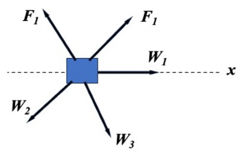
In most of the engineering problems which are related to systems in static equilibrium normally two forces are unknown as shown in Figure 1. The forces $F_1$ and $F_2$ are unknown whereas $W_1$ to $W_3$ are known forces. Let say that the unknown forces are making an angle of $\theta_1$ and $\theta_2$ whereas, the $W_1$ to $W_3$ forces are making angles of $\theta_{w 1}, \theta_{w 2}$, and $\theta_{w 3}$ form the positive $x$-axis, respectively. As the body is in equilibrium under all the forces so the net force along $x$ and its perpendicular direction should add up to zero. On resolving the forces along $x$ and its perpendicular direction following equations are obtained [37]:
$\begin{gathered}F_1 \cos \left(\theta_1\right)+F_2 \cos \left(\theta_2\right)+W_1 \cos \left(\theta_{w 1}\right)+ \\ W_2 \cos \left(\theta_{w 2}\right)+W_3 \cos \left(\theta_{w 3}\right)=0\end{gathered}$ (1)
$\begin{gathered}F_1 \sin \left(\theta_1\right)+F_2 \sin \left(\theta_2\right)+W_1 \sin \left(\theta_{w 1}\right)+ \\ W_2 \sin \left(\theta_{w 2}\right)+W_3 \sin \left(\theta_{w 3}\right)=0\end{gathered}$ (2)
Now rearranging Eqs. (1) and (2) will result in Eqs. (3) and (4) as shown below:
$F_1 \cos \left(\theta_1\right)+F_2 \cos \left(\theta_2\right)=-\sum_{i=1}^{i=N} W_i \cos \left(\theta_{w i}\right)$ (3)
$F_1 \sin \left(\theta_1\right)+F_2 \sin \left(\theta_2\right)=-\sum_{i=1}^N W_i \sin \left(\theta_{w i}\right)$ (4)
where, N is the number of known forces. Now in matrix notation the above equations can be written as:
$\left[\begin{array}{cc}\cos \left(\theta_1\right) & \cos \left(\theta_2\right) \\ \sin \left(\theta_1\right) & \sin \left(\theta_1\right)\end{array}\right]\left[\begin{array}{l}F_1 \\ F_2\end{array}\right]=\left[\begin{array}{l}-\sum_{i=1}^{i=N} W_i \cos \left(\theta_{w i}\right) \\ -\sum_{i=1}^{i=N} W_i \sin \left(\theta_{w i}\right)\end{array}\right]$ (5)
Now this is in a simple matrix form AX=b, which can be easily solved using any of the existing functions present in linear algebra function of NumPy. Here, A, X, and b are as follows:
$\begin{gathered}A=\left[\begin{array}{cc}\cos \left(\theta_1\right) & \cos \left(\theta_2\right) \\ \sin \left(\theta_1\right) & \sin \left(\theta_1\right)\end{array}\right] \\ X=\left[\begin{array}{l}F_1 \\ F_2\end{array}\right] \\ b=\left[\begin{array}{c}-\sum_{i=1}^{i=N} W_i \cos \left(\theta_{w i}\right) \\ -\sum_{i=1}^{i=N} W_i \sin \left(\theta_{w i}\right)\end{array}\right]\end{gathered}$
Figure 1. A typical system in static equilibrium
While classical analytical methods, such as resolving forces and solving linear equations manually provide a clear insight into the static equilibrium, they often become cumbersome and error-prone when dealing with complex force systems or multiple unknowns. Additionally, graphical interpretations and hand calculations can be time-consuming and less flexible for parametric studies or iterative design processes. Python programming addresses these challenges by offering numerical solvers and visualization tools that automate and streamline the analysis. This not only enhances computational efficiency but also reduces human error and allows the engineers and students to focus more on interpretation and design rather than tedious calculations.
To facilitate the solution procedure the following function has been developed:
First the module numpy has to be imported to work with arrays (from numpy import *). In line no. 1, the function is defined with the name Eqli_Eqn_solve which accepts three arguments viz.
In lines 10 to 12 the list of θ_un, W, and θ_w are converted into numpy arrays. As the arguments of trigonometric functions should be in radians, so θ_un and θ_w are converted into radians using function radians()in line 15 and 18, respectively. Then a two-dimensional array (A matrix) is created in line 20 and in lines 21 and 22 the rows are assigned with cosines and sines of respective angles. In line 25, the right-hand side vector b is created and in line 27 and 28 the elements are assigned the values as shown in Eq. (5). Finally, linalg.solve() function has been used to solve $A X=b$ which will return the values of forces $F_1$ and $F_2$.
The choice of the NumPy library is deliberate due to its efficiency and reliability in handling numerical computations involving arrays and matrices, which are essential in solving equilibrium equations. The linalg.solve() function is particularly advantageous as it is optimized for solving linear systems of the form $A X=b$ using LU decomposition, making it more efficient and accurate than writing custom solvers or using basic Python data structures. Compared to alternatives like manually implementing Gaussian elimination or using general-purpose libraries like math, NumPy offers faster performance, better error handling, and compatibility with large-scale scientific computations. This makes it highly suitable for educational and practical applications in engineering analysis.
|
def Eqli_Eqn_solve(θ_un,W,θ_w): ''' This function evaluates the unknown forces in equilibrium Inputs: θ_un-angles for unknown forces W-known force magnitude θ_w-angles of known weight Outputs: Array of unknown forces ''' #converting forces and angles in array W=array(W) θ_un=array(θ_un) θ_w=array(θ_w) # converting unknown force angles in radians θ_un=radians(θ_un) # converting known force angles in radians θ_w=radians(θ_w) # Array creation (Constructing the coefficient matrix A) A=empty((len(θ_un),len(θ_un))) A[0,:]=cos(θ_un[:]) A[-1,:]=sin(θ_un[:]) # RHS vector (Constructing the right-hand side vector b (net known forces)) b=empty(len(θ_un)) b[:]=array([-sum(W[:]*cos(θ_w[:])),-sum(W[:]*sin(θ_w[:]))]) # Solving the linear system A·x = b to find unknown forces return linalg.solve(A,b) |
Now, let us apply the above function on some numerical problems to obtain the unknown forces.
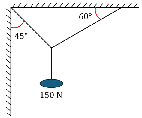
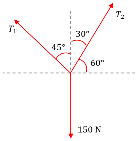
Example 1: A 150 N weight is suspended by two cables (as shown below) attached to a rigid support, forming angles of 45° and 60° with the horizontal. Assuming the system is in static equilibrium, determine the tensions T1 and T2 in the two cables by resolving forces in both the horizontal and vertical directions [37] as shown in Figure 2.
(a) Force developed in wires
(b) Free body diagram (FBD)
Figure 2. Static equilibrium of a suspended mass supported by two cables at different angles
Solution:
|
Main Program |
|
# Input Data # List of unknown force angles (in deg) θ_un=[60,135] # List of known weights (in kN) W=[150] # List of known weights angles (in deg) θ_w=[270] # Calling function to evaluate tensions T1,T2=Eqli_Eqn_solve(θ_un,W,θ_w) print(f"T1[{θ_un[0]}]={round(T1,3)} kN; T2[{θ_un[1]}]={round(T2,3)} kN") |
|
Output |
|
T1[60]=109.808 kN; T2[135]=77.646 kN |
The computed values are $T_1$=109.808 kN at an angle of $60^{\circ}$ and $T_2$=77.646 kN at an angle of $135^{\circ}$. These results indicate that the left cable (corresponding to $T_1$) bears a higher load due to its steeper angle, thereby providing more vertical force to counteract the 150 N weight. The right cable (corresponding to $T_2$) carries a comparatively lower force since its inclination distributes more of the force horizontally rather than vertically. This solution confirms the balance of forces in both axes, ensuring the system remains in equilibrium.
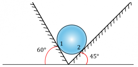
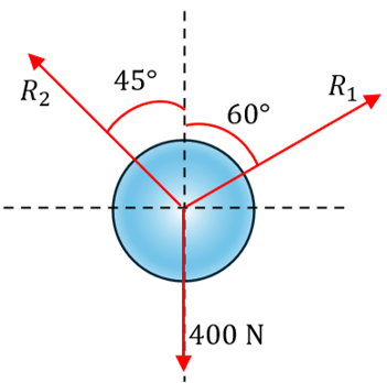
Example 2: A 400 N sphere is resting in equilibrium between two smooth inclined surfaces (as shown below), which form angles of $45^{\circ}$ and $60^{\circ}$ with the horizontal. The sphere experience's normal reaction forces $R_1$ and $R_2$ from the inclined surfaces. Assuming the system is in static equilibrium, determine the magnitudes of the reaction forces $R_1$ and $R_2$ by resolving forces in both the horizontal and vertical directions [37] (see Figure 3).
(a) Sphere on wedge
(b) FBD
Figure 3. Equilibrium of a sphere resting between two inclined surfaces
Solution:
|
Main Program |
|
# Input Data # List of unknown force angles (in deg) θ_un=[270-60,270+45] # List of known weights (in kN) W=[400] # List of known weights angles (in deg) θ_w=[90] # Calling function to evaluate reactions T1,T2=Eqli_Eqn_solve(θ_un,W,θ_w) print(f"T1[{θ_un[0]}]={round(T1,3)} kN; T2[{θ_un[1]}]={round(T2,3)} kN") |
|
Output |
|
R1[210]=292.82 kN; R2[315]=358.63 kN |
The computed values, $R_1$=292.82 kN and $R_2$=358.63 kN, indicate that the reaction force on the right surface $\left(R_2\right)$ is greater, implying that this surface provides more resistance in counteracting the vertical force. The sum of these reaction forces ensures equilibrium by balancing both the vertical and horizontal force components acting on the sphere. The directional angles correspond to the orientation of the inclined surfaces, ensuring the net force in the system remains zero. These results confirm the correct application of equilibrium conditions, reinforcing the balance of forces acting on the sphere.
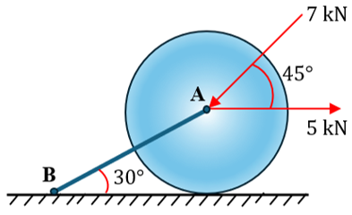
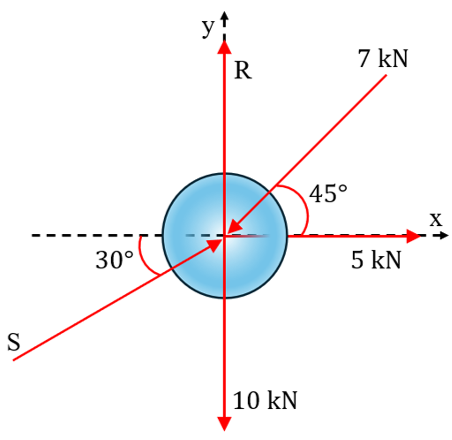
Example 3: A sphere at point A is subjected to three known forces: a 7 kN force acting at a $45^{\circ}$ angle, a 5 kN horizontal force, and a 10 kN vertical downward force. Additionally, the sphere is in contact with bar $(A B)$ at a $30^{\circ}$ angle, which exerts a reaction force $S$. The system is in static equilibrium, with a reaction force $R$ acting at the contact point. Determine the magnitudes of the reaction forces $S$ and $R$ by resolving the forces into horizontal and vertical components. Verify that the sum of forces in both directions is zero, ensuring the equilibrium condition is satisfied [5] as shown in Figure 4.
(a) Sphere on ground and tied by bar CA
(b) FBD
Figure 4. Force analysis of a sphere resting on the ground with an inclined support at point B
Solution:
|
Main Program |
|
# Input Data # List of unknown force angles (in deg) θ_un=[30,90] # List of known weights (in kN) W=[5,-7,10] # List of known weights angles (in deg) θ_w=[0,45,270] # Calling function to evaluate reaction and tension S,R=Eqli_Eqn_solve(θ_un,W,θ_w) print(f"S[{θ_un[0]}]={round(S,3)} kN; R[{θ_un[1]}]={round(R,3)} kN") |
|
Output |
|
S[30]=-0.058 kN; R[90]=14.979 kN |
The computed values, $S$=-0.058 kN and $R$=14.979 kN, indicate that the support reaction along the inclined plane is nearly negligible, implying that the applied forces are primarily balanced by the vertical reaction force $R$. The negative value of $S$ suggests that the assumed direction might be opposite to the actual reaction force or that its contribution is minimal. The significant value of $R$ confirms that most of the equilibrium condition is maintained by the vertical reaction force, effectively counteracting the downward 10 kN force while also accounting for the vertical components of other applied forces.
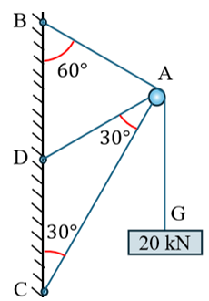
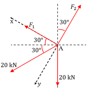
Example 4: A pulley is mounted at point A and is supported by two bars, AB and AC, which are attached to a fixed vertical wall. A cable is hinged at point D and passes over the pulley, supporting a 20 kN load at point G. The angles between the members and the horizontal or vertical directions are given as 30°, 60°, and 30°. Determine the forces $F_1$ and $F_2$ in the supporting members by resolving forces along the x and y directions [5] (see Figure 5).
(a) Arrangement of rope, pully, bar, and weight
(b) FBD
Figure 5. Structure and its free-body diagram showing applied forces and corresponding force components at point A
Solution:
As the pully is frictionless so the tension on the chord AD will be same as the external weight, i.e., 20 kN.
|
Main Program |
|
# Input Data # List of unknown force angles (in deg) θ_un=[90+60,60] # List of known weights (in kN) W=[20,20] # List of known weights angles (in deg) θ_w=[210,270] # Calling function to evaluate tensions F1,F2=Eqli_Eqn_solve(θ_un,W,θ_w) print(f"F1[{θ_un[0]}]={round(F1,3)} kN; F2[{θ_un[1]}]={round(F2,3)} kN") |
|
Output |
|
F1[150]=0.0 kN; F2[60]=34.641 kN |
The calculated results indicate that force $F_1$ along the $150^{\circ}$ direction is zero, meaning that there is no force required in this direction to maintain equilibrium. This is due to the geometric symmetry of the force system about the vertical axis. However, the force $F_2$, acting at $60^{\circ}$, is determined to be 34.641 kN, which balances the applied loads and maintains static equilibrium. This suggests that the system primarily relies on the force in the $60^{\circ}$ direction to support the given loads while no force contribution is needed in the $150^{\circ}$ direction.
Note that in all the examples the forces going away from node are considered. If the forces come to the node, then one can evaluate its angle when it is the opposite side and correspondingly write the angle. Table 1 presents the comparison of the results obtained from Python programming and the one mentioned in the literature for all the examples. The Python results exactly matches with the results found in the literature.
Table 1. Comparison of obtained results with the theory
|
Example |
Theoretical [37] |
From Python Code |
|
1 |
T1[60]=109.8 kN T2[135]=77.6 kN |
T1[60]=109.808 kN T2[135]=77.646 kN |
|
2 |
R1[210]=292.8 kN R2[315]=358.6 kN |
R1[210]=292.82 kN R2[315]=358.63 kN |
|
3 |
S[30]=-0.058 kN R[90]=14.98 kN |
S[30]=-0.058 kN R[90]=14.979 kN |
|
4 |
F1[150]=0.0 kN F2[60]=34.64 kN |
F1[150]=0.0 kN F2[60]=34.641 kN |
Across all examples, it has been observed that the steeper force directions (closer to vertical) bear higher load magnitudes due to their superior capacity to counteract the gravitational forces. Conversely, shallower angles result in lower vertical components, thus smaller tensions or reactions. In symmetric setups, one force can become redundant. These outcomes reinforce classical principles of force resolution and equilibrium, validating the Python-based computational model. Unexpected results, like negative values, often indicate misassumed directions and highlight the importance of the vector interpretations in statics.
While the Python implementation using numpy.linalg.solve() ensures precise and efficient solutions for systems in static equilibrium, some limitations remain. The method assumes ideal conditions such as exact input angles and perfectly known force magnitudes. In real-world applications, measurement errors, incorrect angle estimation, and modeling simplifications (e.g., neglecting friction or assuming point loads) can affect the accuracy of the results. Additionally, if the input angles are not linearly independent (e.g., collinear forces), the system matrix may become singular or ill-conditioned, which would lead to numerical instability or failure in computation.
In this exploration of solving static equilibrium using Python programming, one can venture into the realm where theory and practice converge. Static equilibrium, a cornerstone of physics and engineering, has been dissected and understood through the lens of Python's computational prowess. Through this journey, the essential principles of static equilibrium, discovering how objects and structures remain at rest under the influence of various forces are unraveled. Python, with its libraries and capabilities, has empowered us to go beyond theory and step into practical problem-solving. A function has been developed to model the system in equilibrium and it has been tested on four standard problems. The result of the program exactly matches the results in the literature [37]. Hence, it has been recognized that Python programming provides a bridge between the abstract concepts of equilibrium and the concrete challenges of the physical world. Armed with this knowledge and practical skill set, one can be better equipped to solve static equilibrium problems with confidence and precision, enriching the understanding of the forces that maintain our world in balance.
While the current study focuses on solving static equilibrium problems using Python, several directions can be explored to enhance and extend this work. One potential improvement is integrating symbolic computation using libraries such as SymPy to derive analytical solutions alongside numerical results. Additionally, incorporating graphical visualization tools like Matplotlib and Plotly can help in better interpreting force diagrams and equilibrium conditions. Further, expanding the program's functionality to analyze dynamic equilibrium problems and structural analysis in engineering applications can provide a more comprehensive tool for students and researchers. It is also acknowledged that the present execution assumes a two-dimensional system with exactly two unknowns; extending the code to support three-dimensional force systems and multiple unknowns is a valuable direction for future development to enhance its applicability to real-world engineering problems. Finally, developing an interactive Python-based application or web interface for solving equilibrium problems in real time could make this tool more accessible and user-friendly.
[1] Vasudevan, A., Aanisha, A.C., Mohammad, S.I., Manoharan, R., Raja, N., Oqilat, O., Alshurideh, M.T. (2025). Divided square divisor cordial and Fibonacci prime labeling of theta graphs in Python. Applied Mathematics and Information Sciences, 19(1): 149-159. https://doi.org/10.18576/amis/190113
[2] Mittelstedt, C. (2023). Engineering Mechanics 2: Strength of Materials. Springer. https://doi.org/10.1007/978-3-662-66590-9
[3] Meriam, J.L., Kraige, L.G. (2006). Engineering Mechanics. John Wiley & Sons, Inc.
[4] Carrera, E., Giunta, G., Petrolo, M. (2011). Beam Structures: Classical and Advanced Theories. John Wiley & Sons. https://doi.org/10.1002/9781119978565
[5] Lavarenne, J., Mbengue, A. (2025). SARRA-Py: A Python-based geospatial simulation framework for agroclimatic modeling. SoftwareX, 30: 102145. https://doi.org/10.1016/j.softx.2025.102145
[6] Ullman, D.G. (2002). Toward the ideal mechanical engineering design support system. Research in Engineering Design, 13: 55-64. https://doi.org/10.1007/s00163-001-0007-4
[7] Stein, E. (2014). History of the finite element method – mathematics meets mechanics – Part I: Engineering developments. In the History of Theoretical, Material and Computational Mechanics - Mathematics Meets Mechanics and Engineering. Lecture Notes in Applied Mathematics and Mechanics, Springer, Berlin, Heidelberg. https://doi.org/10.1007/978-3-642-39905-3_22
[8] Alipour, P. (2024). The dual reciprocity boundary element method for one-dimensional nonlinear parabolic partial differential equations. Journal of Mathematical Sciences, 280: 131-145. https://doi.org/10.1007/s10958-023-06642-4
[9] Prajapati, D.K., Prakash, C., Saxena, K., Gupta, M., Mehta, J.S. (2014). Prediction of contact response using boundary element method (BEM) for different surface topography. International Journal on Interactive Design and Manufacturing, 18: 2725-2732. https://doi.org/10.1007/s12008-023-01290-z
[10] Qin, X., Shen, Y., Chen, W., Yang, J., Peng, L.X. (2021). Bending and free vibration analyses of circular stiffened plates using the FSDT mesh-free method. International Journal of Mechanical Sciences, 202-203: 106498. https://doi.org/10.1016/j.ijmecsci.2021.106498
[11] Hoffer, J.G., Geiger, B.C., Ofner, P., Kern, R. (2021). Mesh-free surrogate models for structural mechanic FEM simulation: A comparative study of approaches. Applied Sciences, 11(20): 9411. https://doi.org/10.3390/app11209411
[12] Thangavel, K., Palanisamy, N., Muthusamy, S., Mishra, O.P., Sundararajan, S.C.M., Panchal, H., Loganathan, A.K., Ramamoorthi, P. (2023). A novel method for image captioning using multimodal feature fusion employing mask RNN and LSTM models. Soft Computing, 37: 14205-14218. https://doi.org/10.1007/s00500-023-08448-7
[13] Long, Y.F., Yu, W.S., Pipes, R.B., Forghani, A., Poursartip, A., Gordnian, K. (2022). Simulation of composites curing using mechanics of structure genome based shell model. Composites Part A: Applied Science and Manufacturing, 154: 106766. https://doi.org/10.1016/j.compositesa.2021.106766
[14] Shin, H.V., Porst, C.F., Vouga, E., Ochsendorf, J., Durand, F. (2016). Reconciling elastic and equilibrium methods: For static analysis. ACM Transactions on Graphics, 35(2): 1-16. https://doi.org/10.1145/2835173
[15] Mourad, L., Bleyer, J., Mesnil, R., Nseir, J., Sab, K., Raphael, W. (2021). Topology optimization of load-bearing capacity. Structural and Multidisciplinary Optimization, 64: 1376-1383. https://doi.org/10.1007/s00158-021-02923-1
[16] Tschuchnigg, F., Schweiger, H.F., Sloan, S.W., Lyamin, A.V., Raissakis, I. (2015). Comparison of finite-element limit analysis and strength reduction techniques. Géotechnique, 65(4): 249-257. https://doi.org/10.1680/geot.14.P.022
[17] Zhou, Y., Zhan, H., Zhang, W., Zhu, J., Bai, J., Wang, Q., Gu, Y.T. (2020). A new data-driven topology optimization framework for structural optimization. Computers & Structures, 239: 106310. https://doi.org/10.1016/j.compstruc.2020.106310
[18] Varsha, M., Yashashree, S., Ramdas, D.K., Alex, S.A. (2019). A review of existing approaches to increase the computational speed of the python. International Journal of Research in Engineering, Science and Management, 2(4): 594-598.
[19] Shein, E. (2015). Python for beginners. Communications of the ACM, 58(3): 19-21. https://doi.org/10.1145/2716560
[20] Moruzzi, G. (2020). Python basics and the interactive mode. In Essential Python for the Physicist, Springer, Cham. pp. 1-39. https://doi.org/10.1007/978-3-030-45027-4_1
[21] Srinath, K.R. (2017). Python-The fastest growing programming language. International Research Journal of Engineering and Technology, 4(12): 354-357.
[22] Pawar, P.S., Mishra, D.R., Dumka, P., Pradesh, M. (2022). Obtaining exact solutions of visco-incompressible parallel flows using python. International Journal of Engineering Applied Sciences and Technology, 6(11): 213-217.
[23] Bäcker, A. (2007). Computational physics education with python. Computing in Science & Engineering, 9(3): 30-33. https://doi.org/10.1109/MCSE.2007.48
[24] Rocklin, M., Terrel, A.R. (2012). Symbolic statistics with SymPy. Computing in Science & Engineering, 14(3): 88-93. https://doi.org/10.1109/MCSE.2012.56
[25] Dumka, P., Chauhan, R., Singh, A., Singh, G., Mishra, D. (2022). Implementation of Buckingham’s Pi theorem using Python. Advances in Engineering Software, 173: 103232. https://doi.org/10.1016/j.advengsoft.2022.103232
[26] Kanagachidambaresan, G.R., Manohar Vinoothna, G. (2021). Visualizations. In Programming with TensorFlow. EAI/Springer Innovations in Communication and Computing, Springer, Cham. https://doi.org/10.1007/978-3-030-57077-4_3
[27] Bisong, E. (2019). Matplotlib and Seaborn. Building Machine Learning and Deep Learning Models on Google Cloud Platform. Apress, Berkeley, CA, pp. 151-165. https://doi.org/10.1007/978-1-4842-4470-8_12
[28] Porcu, V. (2018). Matplotlib. Python for Data Mining Quick Syntax Reference, Apress, Berkeley, CA, pp. 201-234. https://doi.org/10.1007/978-1-4842-4113-4_10
[29] Ranjani, J., Sheela, A., Pandi Meena, K. (2019). Combination of NumPy, SciPy and Matplotlib/Pylab-A good alternative methodology to MATLAB-A Comparative analysis. In 2019 1st International Conference on Innovations in Information and Communication Technology (ICIICT), Chennai, India, pp. 1-5. https://doi.org/10.1109/ICIICT1.2019.8741475
[30] Gajula, K., Sharma, V., Sharma, B., Mishra, D.R., Dumka, P. (2022). Modelling of energy in transit using python. International Journal of Innovative Science and Research Technology, 7(8): 1152-1156.
[31] Bauckhage, C. (2020). NumPy/SciPy recipes for data science: Subset-constrained vector quantization via mean discrepancy minimization.
[32] Johansson, R. (2018). Numerical python: Scientific computing and data science applications with NumPy, SciPy and matplotlib, Second edition. Apress, Berkeley, CA. https://doi.org/10.1007/978-1-4842-4246-9
[33] Fuhrer, C., Verdier, O., Solem, J.E., Führer, C., Verdier, O., Solem, J.E. (2021). Scientific computing with Python. In High-Performance Scientific Computing with NumPy, SciPy, and Pandas, Packt Publishing Ltd.
[34] Dumka, P., Chauhan, R., Mishra, D.R., Shaik, F., Govindaraj, P., Kumar, A., Sonawane, C., Velkin, V.I. (2024). Development and implementation of a Python functions for automated chemical reaction balancing. Indonesian Journal of Electrical Engineering and Computer Science, 34(3): 1557-1565. https://doi.org/10.11591/ijeecs.v34.i3.pp1557-1565
[35] Randles, B.M., Pasquetto, I.V., Golshan, M.S., Borgman, C.L. (2017). Using the Jupyter notebook as a tool for open science: An empirical study. In 2017 ACM/IEEE Joint Conference on Digital Libraries (JCDL), Toronto, ON, Canada, pp. 1-2. https://doi.org/10.1109/JCDL.2017.7991618
[36] Kyriakou, F., Maclean, C., Dempster, W., Nash, D. (2020). Efficiently simulating an endograft deployment: A methodology for detailed CFD analyses. Annals of Biomedical Engineering, 48: 2449-2465. https://doi.org/10.1007/s10439-020-02519-8
[37] Bhavikatti, S.S., Rajashekarappa, K.G. (1994). Engineering Mechanics. New Age International.