Salaheddin J. Juneidi*![]() | Rami M. Amro
| Rami M. Amro![]()
© 2025 The authors. This article is published by IIETA and is licensed under the CC BY 4.0 license (http://creativecommons.org/licenses/by/4.0/).
OPEN ACCESS
Vegetables are one of the most daily consumable crops, and mass produced in greenhouses. Several previous experimental scientific studies have reported on the main chemical elements that speed the growth rate and crop amount. While experimental studies are taking a long time to investigate the effect of these chemical elements on the plant and harvest growth. Biophysical modelling which relies on biochemical and biophysical mechanisms can reduce the time and chemical waste, in addition it offers insights to scientists, engineers and farmers at the same time. Moreover, recent advances in Internet of Things (IoT) help to control growth factors such as irrigation, temperature, light intensity, and humidity etc. IoT provides practical solutions to simultaneous measurements of ionic concentration in soil and plants. In this research paper, we have developed a model that consists of a few differential equations that model biochemical and biophysical mechanisms. These equations are significant to predict and to supervise tomato plant’s growth to increase crop production. The model offers experimentally validated predictions, and extrapolates the effect of three main chemical nutrients; Nitrogen, Potassium, and Phosphorus on the life cycle of tomato. The model has the advantage over previous modelling attempts; it uses less number of parameters that are involved directly to plant growth and production. Moreover, it incorporates time explicitly. The model has low dimensionality compared to existing models, yet it reproduces the experimentally observed effects on tomato growth and crop amount.
IoT, Arduino, NPK sensors, modelling, differential equations
Using IoT for modeling Nitrogen (N), Phosphorous (P), and Potassium (K) (NPK) nutrition in planting vegetables can be a beneficial approach. By incorporating IoT devices and sensors into smart green houses, you can collect real-time data on various environmental factors, such as soil moisture, temperature, and light levels [1, 2]. To model NPK nutrition, you can deploy IoT sensors that measure the nutrient levels in the soil. These sensors can provide data on the current nutrient status and help you monitor and optimize the NPK levels for optimal vegetable growth. By connecting these sensors to a central system or platform, you can collect and analyze the data to gain insights into the nutrient levels and make informed decisions about fertilizer application. Additionally, IoT devices can assist in automating the irrigation process based on the measured soil moisture levels. This ensures that plants receive adequate water while avoiding overwatering or under watering, which can impact nutrient availability and uptake. Furthermore, by integrating weather data into your modeling system, you can account for external factors that influence nutrient absorption, such as rainfall patterns and temperature changes. This holistic approach can help you develop a comprehensive model for NPK nutrition in your vegetable garden. Overall, utilizing IoT for modeling NPK nutrition in planting vegetables enables precision agriculture, optimizing nutrient management, and promoting healthier and more productive crops. In previous paper [3], we have seen in practice through data collection the importance of calibrating the amount of nutrients that are important for the plants. This calibration is fully depending on plant’s several growth levels, from plant nursing stage until fruit harvesting stage.
NPK refers to the three major nutrients that are essential for plant’s growth: Nitrogen (N), Phosphorous (P), and Potassium (K). These fertilizers are mostly found in nutrients and soil and used to improve plant growth and crop production.
In the past three decades, nutrient balances from a historical perspective have gained momentum as a way to reach best conclusions about the history and functioning of agro-ecosystems. It combines past information on weather and soils, crop and yield patterns, and key management practices, among other data, with current predictive models of soil nutrient cycling. However, most of the applied models lack one or more important processes, for example, nitrogen leaching or soil weathering, and most efforts have focused on nitrogen homeostasis, ignoring the importance of P and K. Recently, NPK analysis has become the basis of many studies of historical nutrient balances involving most input-output processes. In general, the agro-ecosystem is analyzed as a whole, which includes all land uses in a given area, but some studies have focused on crop yield [4].
Each of the nutrients considered has its own natural and synthetic history, as well as soil-specific soil chemistry. N has a long recent history. The interest devoted to P at present, results largely from its limited global reserves and because it continues to provide key missing links in agricultural history. K has become a “forgotten nutrient” and is not considered as important as N and P, although it plays a major role in plant physiology. Potassium reserves appear to be sufficient for hundreds of years but profitability in marginal soils will increasingly depend on its efficient use [5].
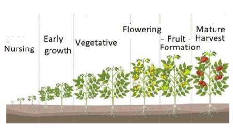
Figure 1. Growing stages of tomato plant last about 100 days [3]
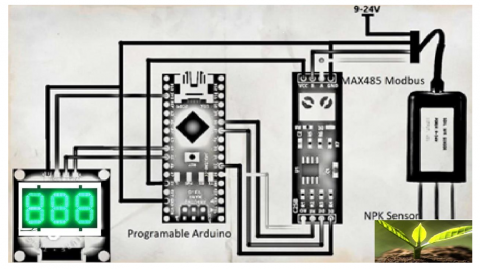
Figure 2. Arduino, NPK sensor and LCD display system to read nutrition in soil [3]
In this study, Figure 1 is defining the growing stages of vegetable plant. Figure 2 is defining the measuring developed tool to read the concentration of NPK in the soil. We examined the soil fertility of agricultural lands using a nutrient balance approach that seeks to cover all NPK inputs and outputs from the topsoil. In the past, where lack of data to determine how much soil needs of NPK nutrition. The agriculture engineers in Palestine were improvising in the most cases, as they do not have a precise measurement tool to determine the concentration of nutrition’s in any area of land, so they had and depend on some common sense of the kind of soil according to the color the soil (e.g., Black Soil, Red Soil, White Soil) [6] and then advise farmers to use fertilizers according this common sense with no precise figures of concentration of each nutrition’s. In Figure 2, we have developed a simple measurement tool that consists of NPK sensor that enables us to determine how much NPK elements in soil with precise figures, then we can determine how much to add of each nutrient concentration. This addition will be added as a solution in the irrigation water. In particular, we found from previous work [3] that N element is mostly needed in first three stages as given in Figure 1, and P element is mostly needed in flowering stage and finally K elements is mostly needed in the last two stages of plant production.
We have defined the three variables as nutrition for a plant, these variables can be gauged by sensors, all of these variables are running by time (100 days) which defined as plant growing and producing stages depicted in Figure 1. Moreover, we can send these readings to be stored as blue-tooth adapter to big data repository [7].
Calibrating NPK levels in soil offers several benefits:
Optimized Nutrient Application: Calibration ensures that you provide the right amount of nutrients, avoiding over-fertilization or under-fertilization, which can negatively impact plant growth and yield.
Cost Savings: Precise nutrient application reduces the wastage of fertilizers, saving you money on unnecessary inputs.
Improved Crop Yield: Properly calibrated NPK levels promote healthy plant growth, leading to increased crop yields and better-quality produce.
Environmental Protection: Accurate nutrient application minimizes nutrient runoff, decreasing the risk of water pollution and environmental harm.
Sustainability: By matching nutrient supply to plant needs, calibration contributes to sustainable agricultural practices and reduces the environmental footprint of farming.
Reduced Nutrient Imbalance: Calibration helps prevent nutrient imbalances that can result in nutrient deficiencies or toxicities, ensuring plants receive a balanced diet for optimal development.
Data-Driven Decisions: Calibration provides data that supports informed decision-making, allowing farmers to adjust nutrient management strategies based on real-time soil and plant conditions.
Enhanced Soil Health: Balancing nutrient levels contributes to soil health, fostering microbial activity and nutrient cycling, which further supports plant growth.
Adaptation to Variability: Different crops and soil types have varying nutrient requirements. Calibration enables tailoring nutrient application to suit the specific needs of each crop and soil type.
Long-Term Productivity: Consistently calibrated NPK levels help maintain soil fertility over time, supporting sustained productivity for future growing seasons.
The main purposes of this study are to develop an integrated nutrient balance model, and to provide a comprehensive assessment of nutrient functions and cycling of past agroecosystems. The proposed model is a build-up and refinement to previous modelling studies [9-12]. In this research article we introduce a model composed of few differential equations as compared to previous studies, albeit it relies on previous modelling and regression models to estimate and simulate some of the needed rates and parameters. Moreover, in contrast to previous models, the modelling methodology here is incorporating the growth time explicitly in the equations which make it easier for implementing it easier parallel to the experiment and by farmers too.
Overall, calibrating NPK levels in soil is a crucial practice that promotes efficient resource utilization, healthier crops, and sustainable agriculture. The research paper is arranged in the following manner: Model description section present model assumption, equations and parameter estimation. Then, in model validation section, we show explain how numerical methodology used to solve the set of differential equations and compare the model output against experimental data provided in reference [3]. Finally, the conclusion and outlook section shed the light on potential future use of the model and how This study would help farmers, researchers and practitioners to have systematic methods based on equations that define the interdependency between NPK as parameters, and the amount to be added to the soil from each N-P-K substance.
Calibrating an NPK equation for soil and vegetables involves determining the appropriate nutrient levels for optimal plant growth. To calibrate, one collects soil samples from the vegetable growing area, conducts nutrient tests, and analyzes the data to establish the relationship between soil nutrient levels (NPK) and plant growth. This helps customize fertilization practices to match the specific nutrient needs of your chosen vegetables.
Several scientific studies have reported on the modelling of vegetable and fruit crops [8-10], such models were also made as available software like Vegsyst, Vegsyst V2 [11], or growth, etc. In These models, a set of differential equations was developed to describe the growth of different organs of the plant. The total growth is the sum of net individual rates of growth in these organs. Other models are dependent on regression analysis which require a pre-knowledge of specific dry matter percentage in each organ [12]. Recent studies have focused on the dynamics of the main ionic concentration in each organ using photo-thermal index [13]. In a less detailed ion uptake studies which was concerned with ion concentration in each organ disregarding the biophysical mechanisms lead to those concentrations, these studies used regression models to estimate the internal ionic concentration, which later used as variables in the dynamical model [9], or in Vegsyst model [10] to estimate the dry matter content of each organ. The studies considered multiple ionic concentrations such as nitrogen, phosphorous, potassium, calcium, magnesium or sulfur. Here, we managed to find a minimal set of equations that take into account regression and dynamical approach to estimate dry and fresh matter based on experimental data provided by Juneidi [3], who has proctored the concentration of three main ionic concentrations, N, P and K, using internet of things techniques measured in units of mg.
We used kinetic rates for photosynthesis of these three main ions in leaves. Starting with base growth rates (Rio, i=N, P, or K) that are calculated using the formula:
Rio=Ro*SLA*Mi
where, Ro is the photosynthesis rate and is dependent on Photosynthesis photon flux density (PPFD). In this model we assume a constant value corresponding to average PPFD level of $R_o \cong 14\mu$mol.m-2.s-1 [14]. Mi is the molar mass of each ion individually in kg units.
Specific leaf area (SLA) was estimated using an exponentially decaying function fitted (R2=0.9) to data in reference [15].
SLA=24.5*(e(-t/330)), with t is simulated in days, SLA has the units of m2/kg.
In general, enzyme activity and hence growth rates are time and temperature dependent [16]. In our model growth rates are assumed to depend on SLA, temperature and internal ionic concentration [17]. Internal ionic concentration is shown to rise monotonically and for simplicity we modelled it logistic growth function [18] a function used widely in modelling plant growth. We model growth rates in the following form with tio=34 days, chosen to be by the end of the germination (nursing and early growth stages) [19]. $\tau_i$=1 day represents the response time for internal ionic concentrations to equilibrate with the external changes in ionic concentrations. lowering $\tau_i$ didn’t affect our results while raising it would make the vegetation process earlier. 0.02 is chosen to reflect basal growth or developmental activity in the germination stage and necessary to reflect non-zero growth.
$R_N=R_{N o} \frac{[N]_{i n}}{1 X 10^{-6}} Q_t *\left(0.02+\frac{1}{1+e^{-\left(\frac{\left(t-t_{N 0}\right)}{\tau_N}\right)^2}}\right)$
$R_P=R_{P o} \frac{[P]_{i n}}{1 X 10^{-6}} Q_t *\left(0.02+\frac{1}{1+e^{\frac{-\left(t-t_{P 0}\right)}{\tau_P}}}\right)$
$R_K=R_{K o} \frac{[K]_{i n}}{1 X 10^{-6}} Q_t *\left(0.02+\frac{1}{1+e^{\frac{-\left(t-t_{K 0}\right)}{\tau_K}}}\right)$
$Q_t$ is the changes in growth rates in response to changes in temperature (T) and is given in terms of the Q10 factor by
$Q_t=Q_{10} \frac{T-T_0}{10}$
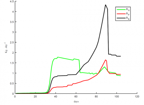
where, Q10 show variations with temperatures, hence we use a regression model in reference [20] for the variations, $Q_{10}=3.22-0.046 * T$, where T is measured in ℃. $[.]_{i n}$ are the internal ion concentrations and calculated using regression models shown below fitted for data in Figure 3 [9] with R2=0.995, given a specific external concentration of the ion $[.]_{\text {ext. }}$
$[N]_{i n}=[N]_{e x t} e^{-t / 130}$
$[P]_{i n}=\frac{[P]_{e x t}}{3.5}$
$[K]_{i n}=\frac{[K]_{e x t}}{2.8}$
Figure 3. Growth rate functions for three main nutrients used in the simulation
We used a system of two differential equations to describe the leaf (WL), fruit (WF) dry matter accumulation, with photosynthesis was done in leaves, the rates in leaves have temperature dependence in addition to concentration and evolution time dependence. We note here, the details of the biophysical mechanisms behind the time evolution of the rates are lumped in sigmoidal like shape (represented by the last terms in parentheses on the right in the RN, RP, and RK formulae) for P, K and Gaussian for N nutrient. The sigmoidal and the gaussian trends are realized from a general growth.
$\frac{d w_L}{d t}=\sum_{i=1}^n B(i) * R_i$ (1)
$\frac{d w_F}{d t}=\sum_{i=1}^n(1-B(i)) * R_i$ (2)
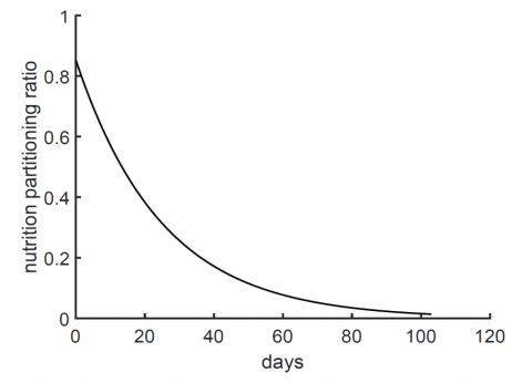
where, the nutrition partitioning function $B(i)=e^{-(t+1.5) / 25}$ having a value between 0 and 1 over growth time course, and accounts for the decline in leaf growth and the rise in the fruit crop. It basically distributes the nutrition material between leaves and fruit. This form of the partitioning function ensures a constant delivery combined percentage of nearly 0.2 (the y-intercept in Figure 4) to the roots and stem as shown in Figure 4 [21]. Moreover, the soaking period of the seeds takes about 1.5 days. The function reasoned to be decreasing at slow rate rather than a sharp decrease to ensure a gradual decrease of the mass allocated to the leaves as compared to the fruit weight which logically should increase with time.
Figure 4. Assumed shape of the nutrition partitioning function as a function of time
To account for harvested mature fruit, we assumed an increasing daily removal rate with a maximal value of 0.135 kg starting from the mature fruit stage which occur around the day 85. Hence, the removed mass ($w_h$) can be modelled as
$\frac{d w_h}{d t}=0.135 /\left(1+e^{\frac{-(t-89)}{0.01}}\right)$ (3)
Eq. (1) describes the accumulation of dry matter in leaves, thus we used this to estimate dry matter in different parts of the plant. For the mass percentage (%N, %P, and %K) of each nutrient in the leaves and fruit respectively, we used percentages provided in reference [21].
Thus, the fresh weight of the leaves, taking into account that most of the fresh mass is water, can be given as
$\mathrm{w}_{\mathrm{L}, { fresh }}=\mathrm{w}_{\mathrm{L}} /(\% \mathrm{~N}+\% \mathrm{P}+\% \mathrm{~K}) * 1 / \mathrm{Wp}_{\mathrm{L}}$ (4)
$\mathrm{w}_{\mathrm{F}, { fresh }}=\mathrm{w}_{\mathrm{F}} /(\% \mathrm{~N}+\% \mathrm{P}+\% \mathrm{~K}) * 1 / \mathrm{Wp}_{\mathrm{F}}$ (5)
Such that, WpL= 1- (%N + %P + %K - % of other dry content in the leaf) is the water percentage in the leaves, and WpF= 1- (%N + %P + %K - % of other dry content in the fruit) is water percentage in fruit. The percentage of other dry content in the leaf and fruit are estimated from reference [21] to be nearly 6% and 2% respectively.
The mass of the stem and root is estimated from fresh mass of the leaves by Eq. (8) and Eq. (9) in reference [9].
$\mathrm{W}_{\mathrm{S}}=0.3391^* \mathrm{~W}_{\mathrm{L}, { fresh }}-0.53771 \times 10^{-3}$ (6)
$\mathrm{W}_{\mathrm{R}}=0.6^* \mathrm{~W}_{\mathrm{L}, { fresh }}$ (7)
Finally, the total mass (Wtot) of the plant is the sum of all the masses carried by each organ of the plant.
$\mathrm{W}_{\text {tot }}=\mathrm{W}_{\mathrm{L}, { fresh }}+\mathrm{W}_{\mathrm{F}, { fresh }}+\mathrm{W}_{\mathrm{R}}+\mathrm{WS}-w_h$
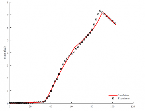
With these equations in hand, we have used MATLAB 2015 to integrate the set of three differential equations using Euler-Maruyama integration scheme with time step 1 day. The dynamical model presented here was able to generate the reported experimental data provided in reference [3] as shown in Figure 5, in which instant measurements of nutrient concentration in the environment were done using IoT. Figure 5 shows that simulation results coincide with experimental observations at most instants of time validating model underlying biophysical assumptions and parameter values. We also notice some near the ripening stage leaving room for future enhancements of the growth rates and the start of the crop cultivation stage. This similarity between the experiment and simulation is attributed to the chosen shape of the growth rates as well other underlying assumptions.
Figure 5. Simulated results and experimental measurements. Simulated data are generated by integrating Eq. (1) using a code written in MATLAB 2015
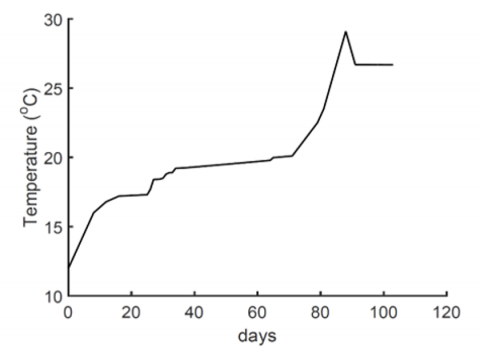
Figure 6. Temperature variation over the 120 days period of planting as used in experiment [3]
The growth rate functions used to generate these results are presented in Figure 3. It is evident that growth rates are strongly influenced by temperature as shown in Figures 3, abrupt changes in temperature are directly reflected in the growth rates (Figures 3 and 6). This observation is consistent with previous experimental findings related to tomato fruit ripening [22]. Growth rates are driven by enzyme activity which we haven’t modelled, rather, the model lump-sum their kinetics in the growth rates and are usually sensitive to abrupt temperature changes [16]. Growth rates are the main driving mechanism in mass production in tomato, hence small changes in their value will result in a direct change to the calculated fresh and dry matter in Eqs. (1) and (2).
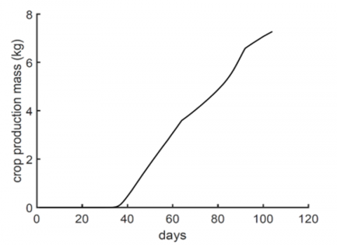
As we can see, the dynamical model, composed of few differential equations, is sufficient to generate the experimentally observed behavior, an advantage over other detailed models which vary in the level of complexity and number of equations. The toy model proposed here is a lump-sum of other models which has many parameters, and uses a different set of regression equations for different tomato organs [9]. Here we see that crop mass can be estimated too, as shown in Figure 7. The simplicity of our model doesn't ignore the internal biophysical mechanisms related to enzyme activity and its time and temperature dependence, instead, we have used growth rate functions that agree with the general shape of them reported in the literature [16]. The exact shape of the growth rates was estimated by choosing physiologically meaningful values such as the approximate starting or ending time of the experimentally observed growth stages [3, 19].
Figure 7. Estimated crop production over time
In this research article, we have developed a biophysical model that incorporate previously published data and models. In this paper we managed to reduce the burden of using many differential equations to estimate the crop mass production, shown in Figure 7. The model basically relies on previous studies on growing and modelling tomato crop in estimating model parameters, either by using average values, or regression curves. The model shows explicit dependence on time as compared to previous models, which account for time implicitly, allowing it to be modified easily for future experiments not only in tomato, but also used as prototype for other crops that have similar life course similar to other previous modelling attempts for cucumber [8] and other fruit-producing greenhouse crops. Thus, our model can be applied to other vegetables albeit model parameters and time period for growth stages are adjusted to reflect the life cycle of the intended plant. The model is based on estimating the fresh mass of the plant as whole, using specific percentages from scientific literature for the abundance of the three main elements (N, P, and K) we are concerned about in this study. The model shows a very reliable way for calculating the total plant weight and crop mass production at any time over the lifespan of the tomato plant. Our results are shown per plant, and can be easily transformed to account for a field of such a plant. The model contains fewer parameters compared to previous attempts at modeling tomato growth. It enables the investigation of the effects of the three main nutrients on growth rate and crop mass production. We observe that nitrogen is essential for vegetative growth and remains a key component of the tomato fruit. Furthermore, the model suggests that after the germination period, the plant initiates a nutrient distribution mechanism, with a time-evolving allocation of the products of the growth process—from the nursing stage to the onset of fruit production.
The model could be improved by incorporating different mass partitioning functions for each growth stage. Additionally, the nutrient percentages in the fruit and leaves are assumed to be constant throughout the model. Future work could explore how variations in these nutrient concentrations impact the total plant mass.
The authors thank Palestine Technical University- Kadoorie for supporting this research.
[1] Laktionov, I.S., Vovna, O.V., Zori, A.A., Lebedev, V.A. (2018). Results of simulation and physical modeling of the computerized monitoring and control system for greenhouse microclimate parameters. International Journal on Smart Sensing and Intelligent Systems, 11(1): 1. https://doi.org/10.21307/ijssis-2018-017
[2] Laktionov, I.S., Vovna, O.V., Zori, A.A. (2017). Planning of remote experimental research on effects of greenhouse microclimate parameters on vegetable crop-producing. International Journal on Smart Sensing and Intelligent Systems, 10(4): 845. https://doi.org/10.21307/ijssis-2018-021
[3] Juneidi, S.J. (2022). Smart greenhouses using internet of things: Case study on tomatoes. International Journal on Smart Sensing and Intelligent Systems, 15(1). https://doi.org/10.2478/ijssis-2022-0019
[4] Ison, J.L.C., San Pedro, J.A.B., Ramizares, J.Z., Magwili, G.V., Hortinela, C.C. (2021). Precision agriculture detecting npk level using a wireless sensor network with mobile sensor nodes. In 2021 IEEE 13th International Conference on Humanoid, Nanotechnology, Information Technology, Communication and Control, Environment, and Management (HNICEM), Manila, Philippines, pp. 1-6. https://doi.org/10.1109/HNICEM54116.2021.9732000
[5] Amrutha, A., Lekha, R., Sreedevi, A. (2016). Automatic soil nutrient detection and fertilizer dispensary system. In 2016 International Conference on Robotics: Current Trends and Future Challenges (RCTFC), Thanjavur, India, pp. 1-5. https://doi.org/10.1109/RCTFC.2016.7893418
[6] Davis, J.N., Pérez, A., Asigbee, F.M., Landry, M.J., et al. (2021). School-based gardening, cooking and nutrition intervention increased vegetable intake but did not reduce BMI: Texas sprouts-a cluster randomized controlled trial. International Journal of Behavioral Nutrition and Physical Activity, 18: 18. https://doi.org/10.1186/s12966-021-01087-x
[7] Juneidi, S.J. (2020). Autonomous data centers ADC: Using agent role locking theory (ARL). International Journal of Advanced Trends in Computer Science and Engineering, 9(4): 5343-5354. https://doi.org/10.30534/ijatcse/2020/169942020
[8] Ramírez-Pérez, L.J., Morales-Díaz, A.B., Benavides-Mendoza, A., De-Alba-Romenus, K., González-Morales, S., Juárez-Maldonado, A. (2018). Dynamic modeling of cucumber crop growth and uptake of N, P and K under greenhouse conditions. Scientia Horticulturae, 234: 250-260. https://doi.org/10.1016/j.scienta.2018.02.068
[9] Juárez-Maldonado, A., Benavides-Mendoza, A., de-Alba-Romenus, K., Morales-Díaz, A.B. (2014). Dynamic modeling of mineral contents in greenhouse tomato crop. Agricultural Sciences, 5(2): 114-123. https://doi.org/10.4236/as.2014.52015
[10] Gallardo, M., Cuartero, J., de la Torre, L.A., Padilla, F.M., Segura, M.L., Thompson, R.B. (2021). Modelling nitrogen, phosphorus, potassium, calcium and magnesium uptake, and uptake concentration, of greenhouse tomato with the VegSyst model. Scientia Horticulturae, 279: 109862. https://doi.org/10.1016/j.scienta.2020.109862
[11] Gallardo, M., Fernández, M.D., Giménez, C., Padilla, F.M., Thompson, R.B. (2016). Revised VegSyst model to calculate dry matter production, critical N uptake and ETc of several vegetable species grown in Mediterranean greenhouses. Agricultural Systems, 146: 30-43. https://doi.org/10.1016/j.agsy.2016.03.014
[12] Gil, R., Bojacá, C.R., Schrevens, E. (2017). A tailor-made crop growth model for the tomato production systems in Colombia. Agronomía Colombiana, 35(3): 301-313. https://doi.org/10.15446/agron.colomb.v35n3.65615
[13] Martinez-Ruiz, A., Sánchez-García, P., Pineda-Pineda, J., Prado-Hernández, J.V., Ruiz-García, A. (2019). Prediction of nitrogen, phosphorus and potassium uptake using a photothermal model. In International Symposium on Advanced Technologies and Management for Innovative Greenhouses: GreenSys2019 1296, pp. 469-476. https://doi.org/10.17660/actahortic.2020.1296.61
[14] Saito, T., Mochizuki, Y., Kawasaki, Y., Ohyama, A., Higashide, T. (2020). Estimation of leaf area and light-use efficiency by non-destructive measurements for growth modeling and recommended leaf area index in greenhouse tomatoes. The Horticulture Journal, 89(4): 445-453. https://doi.org/10.2503/hortj.utd-171
[15] Costa, L.C., Filho, A.B.C., Ribas, R.G.T., Dutra, A.F., Rocha, A.M.S., Barbosa, J.C. (2020). Growth analysis of tomato for industrial processing as a function of nitrogen doses. Australian Journal of Crop Science, 14(8): 1348-1354. https://doi.org/10.21475/ajcs.20.14.08.p2648
[16] Daniel, R.M., Danson, M.J. (2013). Temperature and the catalytic activity of enzymes: A fresh understanding. FEBS Letters, 587(17): 2738-2743. https://doi.org/10.1016/j.febslet.2013.06.027
[17] McIlrath, W.J. (1950). Growth responses of tomato to nutrient ions adsorbed on a pumice substrate. Plant Physiology, 25(4): 682. https://doi.org/10.1104/pp.25.4.682
[18] Latif, N.S.A., Mushoddad, N.A.M.A., Azmai, N.S.M. (2020). Agriculture management strategies using simple logistic growth model. IOP Conference Series: Earth and Environmental Science, 596(1): 012076. https://doi.org/10.1088/1755-1315/596/1/012076
[19] Shamshiri, R.R., Jones, J.W., Thorp, K.R., Ahmad, D., Man, H.C., Taheri, S. (2018). Review of optimum temperature, humidity, and vapour pressure deficit for microclimate evaluation and control in greenhouse cultivation of tomato: A review. International Agrophysics, 32(2): 287-302. https://doi.org/10.1515/intag-2017-0005
[20] Tjoelker, M.G., Oleksyn, J., Reich, P.B. (2001). Modelling respiration of vegetation: Evidence for a general temperature-dependent Q10. Global Change Biology, 7(2): 223-230. https://doi.org/10.1046/j.1365-2486.2001.00397.x
[21] Şahin, M., Tepecik, M., Gül, A., Özaktan, H. (2013). Rhizobacterium affects uptake and distribution of nutrients in tomato plants grown in perlite. Soil-Water, 2(2): 619-626.
[22] Adams, S.R., Cockshull, K.E., Cave, C.R.J. (2001). Effect of temperature on the growth and development of tomato fruits. Annals of Botany, 88(5): 869-877. https://doi.org/10.1006/anbo.2001.1524