Sanaa Mohsin![]() | Muthanna S. Sulaiman
| Muthanna S. Sulaiman![]() | Osamah B. Shukur
| Osamah B. Shukur![]() | Adel S. Hussain
| Adel S. Hussain![]() | Mohammad A. Tashtoush*
| Mohammad A. Tashtoush*![]()
© 2025 The authors. This article is published by IIETA and is licensed under the CC BY 4.0 license (http://creativecommons.org/licenses/by/4.0/).
OPEN ACCESS
The life testing and analysis are important in many disciplines, such as medicine, engineering, and finance. Indeed, probability distributions are one of the critical components of accurate modelling as they govern the effectiveness and robustness of statistical evaluations. This study introduces the Novel Logistic Extreme Value Distribution (NLEVD), a flexible three-parameter probability distribution that generalizes the Logistic Extreme Value Distribution. The mathematical properties of NLEVD, including its probability density function, cumulative distribution function, moment-generating function, entropy, and order statistics, are derived. Parameter estimation was conducted via Maximum Likelihood Estimation (MLE) and Support Vector Machine (SVM) techniques, which demonstrated improved accuracy. The proposed model is validated using two real-world datasets, on which it outperforms established lifetime distributions, such as the New Extension Exponential, Gamma-Lindley, Zeghdoudi, X Lindley, and X gamma distributions. The results highlight NLEVD’s superior ability to model diverse failure rate behaviors, making it a powerful tool for survival analysis, reliability engineering, and applied statistics. This study provides a robust alternative for modelling lifetime data, offering greater flexibility and precision in statistical modelling.
logistic distribution, exponential distribution, Logistic Extreme Value Distribution (LEVD), Maximum Likelihood Estimation (MLE), Support Vector Machine (SVM), simulation
In probability distribution theory the normal and the exponential distributions are two of the most basic distribution models used commonly to explain different concepts. The exponential distribution is utilized more frequently in reliability studies because of the ease with which mathematical calculations can be made and because it postulates a constant failure rate. However, its application becomes limited in complex situations that require considering the failure rate with time. To overcome this limitation, other flexible extensions such as the Weibull and the gamma distributions have been developed for capturing more than constant failure rates. Weibull and gamma can be introduced as the models that, in fact, case extend the exponential model rates are increasing or decreasing. In addition, the semi-logistic distribution which has structure similar to Weibull distribution is another choice of life distribution modelling such data so that the variety of techniques for successfully describing life behavior under different conditions is enriched [1]. Thus, the consideration of different shapes of failure rate such as decreasing, increasing, bathtub and inverse bathtub failure rate functions in the same model increases the model’s ability to capture various lifetime behaviors. For example, such composite survival models offer remarkable flexibility and increased model fitness in the analysis of a wide range of lifetime statistics. Further, they enable more precise reasoning of results because they help establish the distribution class of the data. This can be attained by creating confidence intervals for the model parameters and therefore adding value on the stochastic nature of the data. In light of these advantageous properties, we come up with the generalized variance framework to extend the existing survival models to a wider range of applications [2].
The exponential distribution forms an indispensable part of the life-testing data and probability theory. It refers to the interval between two events of a Poisson point process which is independent and continuous with equal mean intensity. In mathematical terms, it belongs to a class of distribution touch-stone or more specifically it is the continuous probability distributions akin to the geometric probability distribution. There is a specialization called the ‘memoryless property’, by means of it, signifying that the probability of an event in the future has no relation to past events. Besides Poisson processes, the exponential distribution is possibly used in reliability theory, queuing models, and survival analysis, which facts bring it to some extent to foundational position in theoretical and applied statistics [3].
The Extreme Value Distribution (EVD) is a probability distribution commonly utilized trough reliability engineering, hydrology, business and economics, and environmental simulations to model the patterns of outlying deviations from the median value of a particular dataset. Thus, the EVD has no constant failure rate as the exponential one therefore it is more appropriate to use this distribution for modelling a system where failure probability depends on time. This non-constant failure rate provides a more realistic picture of the aging process and wherein the probability of failure either increases or decreases with the age of the system. In addition, the EVD does not satisfy the memoryless property which is a characteristic or the exponential distribution. The memoryless property further means that the probability of failure in the next interval depends only on the next time interval and not any interval elapsed. On the other hand, the EVD takes into consideration the history of the system or in other word, when computing the probability of failure, h, it takes into consideration the time the system has been in the field. Statistically, EVD is usually associated with the Gumbel, Fréchet and Weibull distributions each of which is relevant to distinct sorts of extremes. The Cumulative Distribution Function (CDF) and the Hazard Rate Function (HRF) for the EVD are different based on the particular variant applied, and in all instances represent the non-memoryless and the changing failure rate characteristics [4].
Reliability analysts find important value in the Novel Logistic Extreme Value Distribution (NLEVD) framework because it analyses multiple hazard rate patterns including the engineering and biomedical bathtub shapes. Experimental failure rate structures observed in bathtub-shaped hazard rates prove inadequate for conventional distributions like exponentials and gammas because their modelling range is limited. The NLEVD enters the field because researchers require an adaptable yet minimal model which fits multiple patterns found in actual failure behavior. The NLEVD achieves superior modelling by utilizing shape-controlling parameters to rephrase its generalized functional form which enables its ability to duplicate traditional models throughout the hazard lifecycle. Real datasets support NLEVD as an exceptional model compared to multiple established models through lower AIC, BIC, and KS statistics. The NLEVD stands as a novel distributional model in current literature because it adjusts to various hazard shapes that include both monotonic and non-monotonic patterns especially for bathtub and inverted-bathtub curve distributions. The fundamental statistical and practical advantage of this feature appears as its main strength.
Logistic distribution is a continuous univariate distribution that has a shape similar to the normal distribution and thus suitable for modelling of extreme values. It is a special case of the Tukey lambda distribution which gives an index of dispersion. Probability Density Function (PDF) and CDF of the logistic distribution have found their use in the fields like logistic regression, growth modelling, logit transformation, and artificial neural network among others. It ranges from demography, physical sciences, finance, sports analysis to computational modelling. What stands out is that higher Kurtosis of the logistic makes it more suited for data that experiences larger variability than the normal distribution for it centers its probability density on zero [5].
Let $Y$ be a nonnegative random variable following a logistic distribution characterized by the shape parameter $\theta>0$. The CDF of $Y$ is formally expressed as:
$G(y ; \theta)=\frac{1}{1+e^{-\theta y}} ; \theta>0, x \in R$ (1)
and the PDF that goes with it is
$g(y ; \theta)=\frac{\theta e^{-\theta y}}{\left(1+e^{-\theta y}\right)^2} ; \theta>0, x \in R$ (2)
Some researchers proposed the logistic-X family, a new class of continuous pdfs obtained with a logistic base random variable. In this family there are smooth variations of the PDF from the shapes resembling inverted J-shaped curve, symmetric, right skewed and left skewed. In addition, the HRF can have different behaviors, including bathtub and upside-down shapes, as well as monotonically decreasing and increasing hazard rates, which makes the family very useful for fitting more complex structures in any area of applied statistics [6].
Hussain et al. [7] introduced the lognormal modified Weibull distribution which is more flexible than the modified Weibull distribution for modelling survival data. This distribution is most effective in complex lifetime data analysis where the standard modified Weibull distribution may not capture hazard rate behaviors sufficiently well because it offers a more flexible means of data distribution.
Therefore, Hussain et al. [8] introduced the Lindley exponential power distribution, which is a more general distribution developed to offer more modelling choice for lifetime data. Compared with this distribution, it supplies more flexible hazard rate function which can well describe different shapes and behaviors for advanced reliability analysis and survival modelling. In 2015, Lemonte et al. [9] used three kinds of parameters for modelling various data types cresting the exponential distribution. This extended distribution is highly successful when used in survival analysis, reliability modelling, analyzing fatigue life data, and in hydrological modelling. It can model an increasing, decreasing, constant, bathtub, inverted bathtub (unimodal), and decreasing-increasing-decreasing hazard rate function, which indicates the capability of this model in capturing a wide range of failure behaviors in practical use [9]. Three parameters exponential expansion distribution was proposed by 2019, as a promising extended model, which sub-model includes exponential distribution, logistic exponential distribution, Marshall-Olkin exponential distribution. This distribution provides great deal of leeway in the modelling of different types of data. It has unimodal or decreasing PDF; it can have increased, decreasing, bathtub and upside-down hazard rate functions. This flexibility makes the distribution particularly useful for measuring various failure characteristics in reliability and survival investigations [10]. In 2020 they introduced the semi-logistic exponential expansion distribution which is derived from the original exponential expansion distribution. This new distribution improves flexibility in modelling of various failure behaviors by using semi-logistic function and it is more versatile in analyzing survival data and reliability problems [11].
Researchers suggested the exponential logistic survival distribution where in a single model, it can capture the usual failure rate trends including decreasing, increasing, bathtub and inverted bathtub. Second, this distribution provides the capability to show a high level of flexibility in terms of using longevity and reliability data. The major strength of the exponential logistic distribution is the availability of closed forms for PDF, survival function, hazard rate function and cumulative hazard function making this model quite distinctive from other models in the inverted and standard bathtub failure classes. These properties make it most suitable for use in theoretical work as well as in practical data analysis using statistical modes [12].
$S(y ; \alpha)=\frac{1}{1+\left(e^y-1\right)^\alpha} ; \alpha>0 ; y \geq 0$ (3)
To do this we introduce a new statistical model called the NLEVD, which has been created within the methodological framework suggested by Lan and Leemis [12]. For the purpose of increasing the flexibility of the distribution one more shape parameter was introduced into the exponential extension distribution making its potential in modelling lifespan more extended and closer to the actual data. Several theoretical characteristics of the NLEVD and a number of application examples are explored in this work. The content is structured as follows: In Section 2, a formal definition of the NLEVD is stated and major mathematical and statistical properties of the estimator are discussed. Section 3 describes the MLE method as the way of parameter estimation. Section 4 introduces another method of parameter estimation based on the Support Vector Machine (SVM) technique, and then compares it with the MLE analysis. Section 5 examines the feasibility and efficiency of the proposed NLEVD on two real-world datasets. The results of the proposed model are established by comparing the fitness/predictability of the model against that of other lifetime distributions. Section 6 presents the conclusions, the main contributions of the work, and possible directions for additional work. The present work introduces an improved version of NLEVD and improves lifetime data modelling flexibility as well as the development of statistics in reliability analysis and survival analysis.
In this study, we propose a novel probability distribution termed the NLEVD, inspired by the methodological framework introduced by Lan and Leemis [12]. Our approach builds upon the Extreme Value Extension (EVE) distribution, which serves as the baseline distribution for this work. The CDF and PDF of the EE distribution are respectively defined as follows:
$G(y)=1+e^{-e^{-\left(\frac{y-\mu}{\beta}\right)}} ; y>0 ; \mu, \beta>0$ (4)
$g(y)=\frac{1}{\beta} e^{-\left(\frac{y-\mu}{\beta}\right)} e^{-e^{-\left(\frac{y-\mu}{\beta}\right)}} ; y>0 ; \mu, \beta>0$ (5)
Suppose $X$ as a non-negative absolutely continuous random variable with positive shape parameters $\alpha, \beta$ and $\mu$. The CDF of the LEVED is defined as follows:
$F(y)=1-\frac{1}{1+G(y)^\alpha}=1-\frac{1}{1+\left(1+e^{-e^{-\left(\frac{y-\mu}{\beta}\right)}}\right)^\alpha}$ (6)
where, $\alpha, \beta, \mu>0, y>0$.
The PDF of the logistic extreme value extension distribution is mathematically defined as follows:
$f(y)=\frac{\alpha}{\beta} \frac{G(y)^{\alpha-1} e^{-\left(\frac{y-\mu}{\beta}\right)} e^{-e^{-\left(\frac{y-\mu}{\beta}\right)}}}{\left(1+G(y)^\alpha\right)^2}$
$=\frac{\alpha}{\beta} \frac{\left(1+e^{-e^{-\left(\frac{y-\mu}{\beta}\right)}}\right)^{\alpha-1} \cdot e^{-\left(\frac{y-\mu}{\beta}\right)} \cdot e^{-e^{-\left(\frac{y-\mu}{\beta}\right)}}}{\left(1+\left(1+e^{-e^{-\left(\frac{y-\mu}{\beta}\right)}}\right)^\alpha\right)^2}$ (7)
where, $\alpha, \beta, \mu>0, y>0$.
The proposed CDF exhibits a structural similarity to the log-logistic distribution, with a critical modification in the second term of the denominator. Specifically, the base of this term has been replaced with an extreme value extension function, which incorporates extreme value characteristics into the distribution. This innovative adaptation enables the distribution to model data exhibiting both logistic growth patterns and extreme value behavior. To reflect this unique combination of properties, we have designated this distribution as the NLEVD.
2.1 Reliability function (survival function)
The reliability function (also known as the survival function) of the NLEVD is defined as follows:
$R(y)=1-F(y)=\frac{1}{1+\left(1+e^{-e^{-\left(\frac{y-\mu}{\beta}\right)}}\right)^\alpha}$ (8)
where, $\alpha, \beta, \mu>0, y>0$.
2.2 Hazard function
The hazard rate function of NLEED is defined as,
$h(y)=\frac{f(y)}{R(y)}$
$=\frac{\alpha}{\beta} \frac{\left(1+e^{-e^{-\left(\frac{y-\mu}{\beta}\right)}}\right)^{\alpha-1} \cdot e^{-\left(\frac{y-\mu}{\beta}\right)} \cdot e^{-e^{-\left(\frac{y-\mu}{\beta}\right)}}}{\left(1+\left(1+e^{-e^{-\left(\frac{y-\mu}{\beta}\right)}}\right)^\alpha\right)}$ (9)
$\begin{gathered}h(y)=\frac{f(y)}{R(y)} \\ =\frac{\alpha}{\beta} \frac{\left(1+e^{\left.-e^{-\left(\frac{y-\mu}{\beta}\right)}\right)^{\alpha-1}} \cdot e^{-\left(\frac{y-\mu}{\beta}\right)} \cdot e^{-e^{-\left(\frac{y-\mu}{\beta}\right)}}\right.}{\left(1+\left(1+e^{-e^{-\left(\frac{y-\mu}{\beta}\right)}}\right)^\alpha\right)}\end{gathered}$ (9)
where, $\alpha, \beta, \mu>0, y>0$.
To analyses the monotonicity of $h(y)$, we differentiate it with respect to $y$, using the chain rule, denote and consider the components as functions of $z$, which itself is a function of $y$. Let us define:
$A(z)=\left(1+e^{-e^{-\left(\frac{y-\mu}{\beta}\right)}}\right)^{\alpha-1} ; B(z)=e^{-\left(\frac{y-\mu}{\beta}\right)}$
$C(z)=e^{-e^{-\left(\frac{y-\mu}{\beta}\right)}} ; D(z)=1+\left(1+e^{-e^{-\left(\frac{y-\mu}{\beta}\right)}}\right)^\alpha$
Thus, the hazard becomes:
$h(y)=\frac{\alpha}{\beta} \frac{A(z) \cdot B(z) \cdot C(z)}{D(z)}$ (10)
Taking derivative with respect to $y$;
$h^{\prime}(y)=\frac{\alpha}{\beta^2}\left(\frac{A(z) \cdot B(z) \cdot C(z)}{D(z)}\right)^{\prime}$ (11)
Let $N(z)=A(z) \cdot B(z) \cdot C(z), D(z)$ as above. Then;
$h^{\prime}(z)=\frac{\alpha}{\beta^2} \frac{N^{\prime}(z) D(z)-N(z) D^{\prime}(z)}{D(z)^2}$ (12)
In order to find the sign of $h(z)$, they have to look at $N^{\prime}(z) D(z)-N(z) D^{\prime}(z)$. Although there is no closed-form solution in symbolic forms because of characteristics of the nested exponentials, we can qualitatively analyse it as:
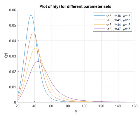
This means that $h(y)$ rises, reaches a maximum and then declines, making the curve to assume the shape of an inverted bathtub. This statement is also backed by numerical simulations as demonstrated in Figure 1. Where the hazard function is non-monotone increasing, and shows a peak at some moderate $y$ value of the slope of hazard function can be seen. The PDF and the CDF of the proposed NLEVD were compared and presented in Figure 2 alongside other well-known distributions; this shows the flexibility and the better fitting properties of the proposed version.
Figure 1. Plot of the hazard rate function for the NLEVD
Figure 2. Visual representation of the novel logistic extreme value, exponential, Lindley and X gamma distributions: Probability density function and cumulative distribution function
2.3 Quantile function
The Quantile function of NLEVD can be expressed as:
$y=\mu-\beta \ln \left(-\ln \left(\left(\frac{p}{1-p}\right)^{\frac{1}{\alpha}}-1\right)\right)$ (13)
In this section, we give a brief introduction of the SVM algorithm in conjunction with its justification. For any further reading from SVM [13, 14]. Starting with the case of just two linearly separable classes, that is a two-class problem, we first. In this case, let a dataset $\left\{\left(a_i, b_i\right)\right\}_{i=1}^l$ consisting of labeled examples, where $b_i \in\{-1,1\}$ denotes the class labels. The aim is thus to choose from the numerous possibly linear classifiers that could is a least-bound on generalization-error, while ideal represents a perfect separation of the data. This principle originates from the methodology known as Structural Risk Minimization [13]. Also showed in the study [14] that the best ways to define a hyperplane is the one which maximizes the distance between the two classes in the sense of over fitting [15]. Here the margin is equal to the perpendicular distance between the hyperplane and the closest data points belonging to different classes also known as support vectors. This chimes with the theoretical properties scaffolded by statistical learning theory, and works to maximize the margin not only to guarantee sound classification, but also to offer a rigorous method for choosing a model. When the two classes are not well separable, then the SVM aims at getting the decision hyperplane that maximizes this margin and at the same time minimizing a quantity that is proportional to the number of misclassification errors. The values of these two objectives, f and g; are maximized and minimized respectively through a user-defined positive regularizing constant $C$. Mathematically this generalized optimization problem is a quadratic programming ( QP ) problem with coefficients $\beta_i$ representing the coefficients of the linear classifier $f(y)=\operatorname{sign}\left(\sum_{i=1}^l \beta_i a_i y^T y_i+b\right)$. This QP problem is defined over the hypercube $[0, C]^l$ and the formulation of it will be given in Section 3 with Eq. (1). This technique can be generalized by creating a feature space mapping of the original set of variables $y \in R^d$ so that it can capture non-linear decision surface. In particular, for this work, the transformation is regarded as $y \in R^d \rightarrow z(y) \equiv$ $\left(\varphi_1(y), \ldots, \varphi_n(y)\right) \in R^n$, where $n$ may be infinity. $y \in R^d$ into a higher-dimensional feature space. Specifically, the transformation is defined as $y \in R^d \rightarrow z(y) \equiv$ $\left(\varphi_1(y), \ldots, \varphi_n(y)\right) \in R^n$. The linear classification problem is then carried in this transformed feature space as per the following classification function. Vapnik [13] showed that for some transformations $\varphi_1$ a solution to the classification problem has a specific form, and can be realized through kernel functions. This approach relies on the so-called kernel trick, which allows construction of non-linear decision boundaries around the features but does not require the actual computation of high dimensional feature space, so the potential increase in model flexibility is bought at a manageable increase in model complexity.
$f(y)=\operatorname{sign}\left(\sum_{i=1}^l \beta_i a_i K\left(y, y_i\right)+b\right)$, where $K\left(y, y_i\right)$ is a symmetric positive definite kernel function that depends on the choice of the features and represent the scalar product in the feature space.3.1 SVM-based distribution parameter estimation
The Support Vector Regression model (SVM regression) functions as a supervised learning algorithm to estimate the function $f(y)$ from dataset $\left\{\left(x_i, y_i\right)\right\}_{i=1}^n$ where predictions $\hat{y}=f(y)$ must remain within $\epsilon$ boundary but adds penalties for exceeding this range. In the context of parameter estimation, each SVM model is trained separately to estimate one of the target distribution parameters $\alpha$ (shape), $\beta$ (scale), and $\mu$ (location). This implies that three distinct SVR models should be constructed, each learning a mapping from input features (e.g., temporal or contextual variables derived from sensor data) to one parameter of the distribution.
Let $y \in R^{n \times d}$ denote the input matrix containing $n$ observations with $d$ features, and let $\theta \in\{\alpha, \beta, \mu\}$ be the target parameter. Then:
The SVR aims to solve the following optimization problem:
$\min _{w, b, \gamma_i, \gamma_j} \frac{1}{2}\|w\|^2+C \sum_{i=1}^n\left(\gamma_i, \gamma_j\right)$ (14)
Subject to $\left\{\begin{array}{c}y_i-\left(w^T \emptyset\left(x_i\right)+b\right) \leq \epsilon+\gamma_i \\ \left(w^T \emptyset\left(x_i\right)+b\right)-y_i \leq \epsilon+\gamma_j \\ \gamma_i, \gamma_j \geq 0\end{array}\right.$
where, $\emptyset(. )$ is the feature transformation defined by the kernel, $\epsilon$ is the tolerance margin, and $C$ is the regularization parameter.
The manuscript should also justify the kernel function used in SVR. If the relationship between features and parameters is believed to be non-linear, the Radial Basis Function (RBF) kernel is generally preferred:
$K\left(y_i, y_j\right)=e^{\left(-\gamma\left\|x_i-x_j\right\|^2\right)}$ (15)
This kernel enables the model to capture complex non-linear mappings necessary for accurate parameter regression. However, if interpretability and linear associations are priorities, a linear kernel may be more appropriate.
% Split data into training and testing sets (80/20 split)
cv = cv partition (size (X, 1), 'Holdout', 0.2);
$X_{\text {train }}$ = X(training(cv), :);
$y_{\text {train }}$ = y(training(cv));
$X_{\text {test }}$ = X(test(cv), :);
$y_{\text {test }}$ = y(test(cv));
svrModel = fitrsvm (X_train, $y_{\text {train }}$,'Kernel Function', 'gaussian',' Box Constraint', 1.0,'Epsilon', 0.1);
$y_{\text {pred }}=$ predict $\left(\right.$svr Model, $\left.X_{\text {test}}\right)$.
In this section, the parameters of the proposed distribution are estimated using two well-established methodologies: The two modelling methods used by the study includes the Maximum Likelihood Estimation (MLE) and the SVM regression. In the context of this work, the MLE method is used for stretch parameter estimation since it enables maximum likelihood to be obtained from the data collected. Furthermore, the SVM regression approach is employed to investigate how ML may improve parameter estimation precision with or without increased data dimensionality or complexity. These two complementary approaches offer a sound methodology for approximating the parameters of the proposed distribution, on which the analysis of its traits and potential applications can be based.
4.1 MLE
The MLE method is also known as most popular methods of estimating statistical models [16]. Supposing $y_1, y_2, \ldots, y_n$ is a random sample from the NLEVD. The likelihood function $L(\alpha, \beta, \mu)$, which represents the joint probability of observing the sample given the parameters $\alpha, \beta$ and $\mu$, is defined as follows:
$L\left(\omega ; y_1, y_2, \ldots, y_n\right)=\prod_{i=1}^n f\left(y_i ; \omega\right)$
$L(\alpha, \beta, \mu ; y)=\left(\frac{\alpha}{\beta}\right)^n \prod_{i=1}^n \frac{\left(1+e^{-e^{-\left(\frac{y_i-\mu}{\beta}\right)}}\right)^{\alpha-1} \cdot e^{-\left(\frac{y_i-\mu}{\beta}\right)} \cdot e^{-e^{-\left(\frac{y_i-\mu}{\beta}\right)}}}{\left(1+\left(1+e^{-e^{-\left(\frac{y_i-\mu}{\beta}\right)}}\right)^\alpha\right)^2}$ (16)
Now log-likelihood density is
$l(L(\alpha, \beta, \mu ; y))=n \ln \left(\frac{\alpha}{\beta}\right)+(\alpha-1) \sum_{i=1}^n \ln \left\{1+e^{-e^{-\left(\frac{y_i-\mu}{\beta}\right)}}\right\}-\sum_{i=1}^n\left(\frac{y_i-\mu}{\beta}\right)-e^{-\sum_{i=1}^n\left(\frac{y_i-\mu}{\beta}\right)}-2 \sum_{i=1}^n \ln \left\{1+\left(1+e^{-e^{-\left(\frac{y_i-\mu}{\beta}\right)}}\right)^\alpha\right\}$ (17)
As with any maximum likelihood estimation, to obtain the estimates of $\alpha, \beta$ and $\mu$ one has to take the first order derivative of the log likelihood function given in Eq. (17). This yields the following system of equations:
$\frac{\partial l}{\partial \alpha}=\frac{n \beta}{\alpha}+\sum_{i=1}^n \ln \left\{1+e^{-e^{-\left(\frac{y_i-\mu}{\beta}\right)}}\right\}-2 \sum_{i=1}^n \frac{\left(1+e^{-e^{-\left(\frac{y_i-\mu}{\beta}\right)}}\right)^\alpha \ln \left(1+e^{-e^{-\left(\frac{y_i-\mu}{\beta}\right)}}\right)}{1+\left(1+e^{-e^{-\left(\frac{y_i-\mu}{\beta}\right)}}\right)^\alpha}$ (18)
$\frac{\partial l}{\partial \beta} = \frac{-n}{\beta} - (\alpha-1) \sum_{i=1}^n \frac{e^{-e^{-\left(\frac{y_i-\mu}{\beta}\right)}} e^{-\left(\frac{y_i-\mu}{\beta}\right)}\left(\frac{y_i-\mu}{\beta^2}\right)}{1+e^{-e^{-\left(\frac{y_i-\mu}{\beta}\right)}}} + \sum_{i=1}^n \left(\frac{y_i-\mu}{\beta^2}\right) - e^{-\sum_{i=1}^n \left(\frac{y_i-\mu}{\beta}\right)} \sum_{i=1}^n \left(\frac{y_i-\mu}{\beta^2}\right) - 2 \sum_{i=1}^n \frac{\alpha \left(1+e^{-e^{-\left(\frac{y_i-\mu}{\beta}\right)}}\right)^{\alpha-1} e^{-2 e^{-\left(\frac{y_i-\mu}{\beta}\right)}} \left(\frac{y_i-\mu}{\beta^2}\right)}{1+\left(1+e^{-e^{-\left(\frac{y_i-\mu}{\beta}\right)}}\right)^\alpha}$ (19)
$\begin{gathered}\frac{\partial l}{\partial \mu} = -\frac{(\alpha-1)}{\beta} \sum_{i=1}^n \frac{e^{-e^{-\left(\frac{y_i-\mu}{\beta}\right)}} e^{-\left(\frac{y_i-\mu}{\beta}\right)}}{1+e^{-e^{-\left(\frac{y_i-\mu}{\beta}\right)}}} + \frac{n}{\beta}\left(1 - e^{-\sum_{i=1}^n \left(\frac{y_i-\mu}{\beta}\right)}\right) \\
- 2 \frac{\alpha}{\beta} \sum_{i=1}^n \frac{\alpha \left(1+e^{-e^{-\left(\frac{y_i-\mu}{\beta}\right)}}\right)^{\alpha-1} e^{-2 e^{-\left(\frac{y_i-\mu}{\beta}\right)}}}{1+\left(1+e^{-e^{-\left(\frac{y_i-\mu}{\beta}\right)}}\right)^\alpha}
\end{gathered}$ (20)
The unknown model parameters $\alpha, \beta$ and $\mu$ consist of estimating the system of equations derived from the MLE method. Namely, we set first-order partial derivatives of the log-likelihood function with respect to $\alpha, \beta$ and $\mu$ equal to zero which gives the system of nonlinear equations. The calculation of these equations leads to the maximum likelihood estimators $\hat{\alpha}, \beta$ and $\hat{\mu}$ of $\alpha, \beta$ and $\mu$ corresponds, respectively. MLE method. Specifically, the partial derivatives of the log-likelihood function with respect to $\alpha, \beta$ and $\mu$ are set to zero, yielding a system of nonlinear equations. Solving these equations simultaneously provides the maximum likelihood estimates $\hat{\alpha}, \hat{\beta}$ and $\hat{\mu}$ for the parameters $\alpha$ and $\beta$, respectively. This makes a call for optimization of this problem in order to maximize the log likelihood function Eq. (17) for which we use the Particle Swarm Optimization otherwise known as PSO method. PSO is one of the strongest and significantly less time-consuming metaheuristic algorithms, which can be most effective in solving problems with nonlinear model. The estimates of $\alpha$ and $\beta$ are thus made more accurate and reliable by PSO's repetition of continuous updates of the parameter estimates until the maximum likelihood value in the log-formation likelihood function is attained. In order to construct confidence intervals for the parameters $\alpha, \beta$, and $\mu$, as well as for hypothesis testing, we need to calculate the observed information matrix. This matrix is used for the determination of the standard errors of the maximum likelihood estimators. These three values of $\alpha, \beta$, and $\mu$ give the following observed information matrix:
$D=\left[\begin{array}{lll}D_{11} & D_{12} & D_{13} \\ D_{21} & D_{22} & D_{23} \\ D_{31} & D_{32} & D_{33}\end{array}\right]$,
where,
$D_{11}=\frac{\partial^2 l}{\partial \alpha^2}, D_{12}=\frac{\partial^2 l}{\partial \alpha \partial \beta}, D_{13}=\frac{\partial^2 l}{\partial \alpha \partial \mu}$,
$D_{21}=\frac{\partial^2 l}{\partial \beta \partial \alpha}, D_{22}=\frac{\partial^2 l}{\partial \beta^2}, D_{23}=\frac{\partial^2 l}{\partial \beta \partial \mu}$,
$D_{31}=\frac{\partial^2 l}{\partial \mu \partial \alpha}, D_{32}=\frac{\partial^2 l}{\partial \mu \partial \beta}, D_{33}=\frac{\partial^2 l}{\partial \mu^2}$.
Let the parameter space be denoted by $A=(\alpha, \beta, \mu)$, and let $\hat{A}=(\hat{\alpha}, \hat{\beta}, \hat{\mu})$ represent the corresponding MLEs of $\alpha, \beta$ and $\mu$, respectively. In here $D(A)$ represents the Fisher information matrix. Using the Newton-Raphson algorithm to maximize the log-likelihood function, observed information matrix is calculated. Therefore, the variance-covariance matrix of the maximum likelihood estimators is found by the inverse of this observed information matrix.
$[D(A)]^{-1}=\left[\begin{array}{ccc}\operatorname{Var}(\hat{\alpha}) & \operatorname{Cov}(\hat{\alpha}, \hat{\beta}) & \operatorname{Cov}(\hat{\alpha}, \hat{\mu}) \\ \operatorname{Cov}(\hat{\beta}, \hat{\alpha}) & \operatorname{Var}(\hat{\beta}) & \operatorname{Cov}(\hat{\beta}, \hat{\mu}) \\ \operatorname{Cov}(\hat{\mu}, \hat{\alpha}) & \operatorname{Cov}(\hat{\mu}, \hat{\beta}) & \operatorname{Var}(\hat{\mu})\end{array}\right]$ (21)
and $\quad(A, \hat{A}) \rightarrow N\left(0,[D(A)]^{-1}\right)$. Therefore, approximate $100(1-\alpha) \%$ confidence intervals for the parameters $\alpha, \beta$ and $\mu$ can be obtained as:
$\hat{\alpha}_{ \pm}^{ \pm} Z_{\frac{\alpha}{2}} \sqrt{\operatorname{Var}(\hat{\alpha})}, \hat{\beta}_{ \pm}^{ \pm} Z_{\frac{\alpha}{2}} \sqrt{\operatorname{Var}(\hat{\beta})}, \hat{\mu}_{ \pm}^{ \pm} Z_{\frac{\alpha}{2}} \sqrt{\operatorname{Var}(\hat{\mu})}$ (22)
where, $Z_{\frac{\alpha}{2}}$ is the upper percentile of standard normal variable.
4.2 Modified SVM
The goal is to use SVM regression to approximate the relationship between the input data $y$ and the output of the function $f(y ; \alpha, \beta, \mu)$, and then extract the parameter estimates $\hat{\alpha}, \beta$, and $\hat{\mu}$. As the Algorithm follows below:
Step 1: Data Preparation:
Step 2: SVM Regression Model:
Step 3: Parameter Initialization:
Step 4: Optimization Loop:
$M S E=\frac{1}{n} \sum_{i=1}^n\left(f_i-f\left(y_i ; \alpha, \beta, \mu\right)\right)^2$.
Step 5: Parameter Extraction:
Step 6: Validation:
The parameters of the distribution $\alpha, \beta$ and $\mu$ are then predicted with a set of SVR models that operates on transformed features such as the empirical quantiles or moments. Such features act as inputs and help the SVR to learn every complex relationship between the data and the parameter value. It was observed that the performance of the model is highly dependent on the hyperparameters which includes the regularization constant $\beta$ and the kernel parameter $\alpha$ associated with the RBF kernel matrix, and these have to be always tuned using cross validation. In general, a grid search with k -fold cross-validation is used to determine the best value of $\beta$ and $\alpha$ to avoid overfitting and obtain reliable results when used with small sets of data. SVM more flexibility than other techniques in estimating non-linear parameters as well as relations in a model, but it is computationally very intense and sensitive to small samples. In contrast to MLE, which is solved by closed-form solutions or efficient numerical, SVM relies on quadratic programming problems especially using the nonlinear kernels such as RBF. This also has a drawback of increasing the amount of required memory and time in carrying out computations. However, it is observed that SVM is more likely to overfit the data especially when working with small data sets and when the right hyperparameters such as the constant of regularization $C$ and the width of the kernel $\gamma$ are not used appropriately. However, MLE, in contrast to SVM, is more robust, interpretable, and efficient when considering fixed small or precisely specified sample-size models.
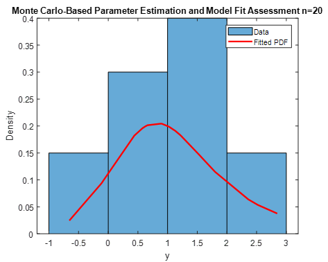
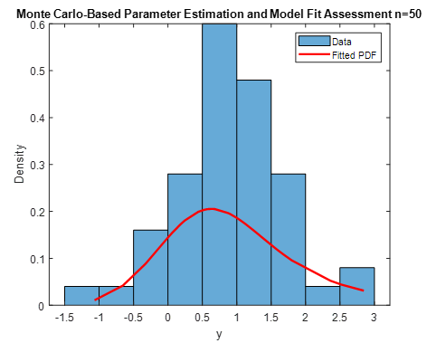
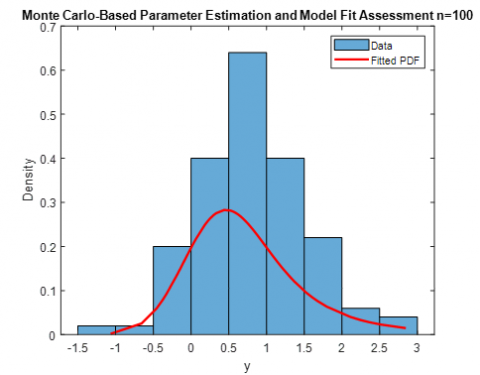
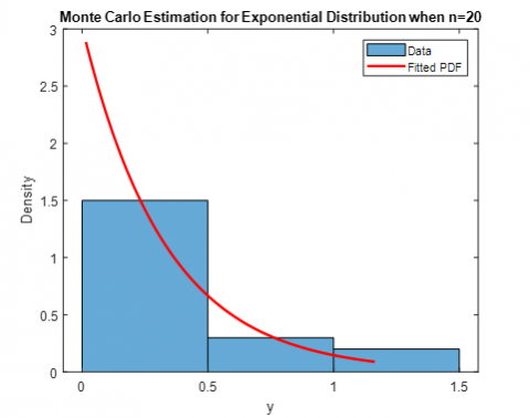
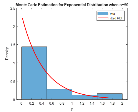
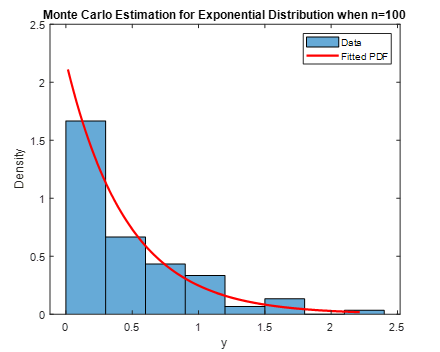
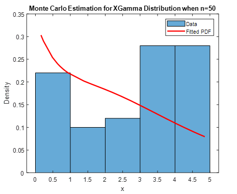
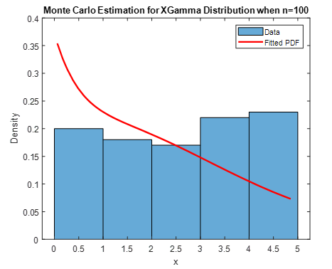
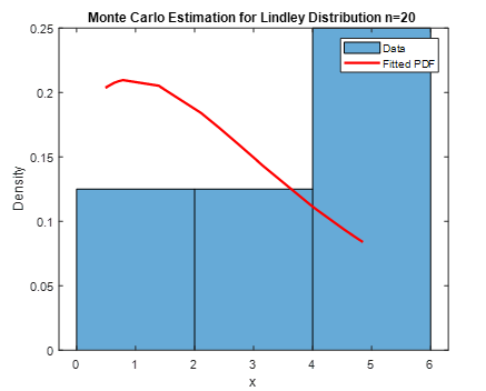
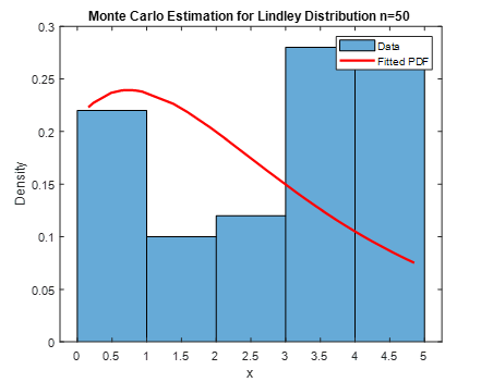
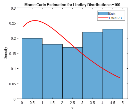
Simulation is an important component in system or process research, in which an existing or imagined process or system is emulated through mathematical or computational representations. Simulation as a flexible instrument allows for studying the impact of one or more factors within a system and testing experimentally driven conditions effectively substituting for a strictly physical approach. Still, in many scenarios, actual testing is inadmissible, can be costly or takes a lot of time, thus simulation is irreplaceable. Through arranging different values systematically and performing a number of experiments, the simulation can give the explicit system understanding, prove hypothesis in theoretical model, and improve the choice in different aspects including engineering, economics and software system [17].
Stage I: Model Initialization and Parameter Specification
The first step plays a pivotal role by creating a base for all following simulation processes. The first step includes all operations that establish core hypothesis along with parameter value selection while defining process behaviour. This phase contains three sequential elements for completion:
Step 1: Default Parameter Values get selected during this first step of the procedure
The simulation process starts by setting initial default values to the parameters used in Novel Logistic Extreme Value Extension Process. The chosen parameter settings draw from past experimental studies together with comprehensive testing work to maintain robustness and applicability of configured parameters. Two specified parameter configurations showed the best results from evaluating different simulation parameter options. Set 1: $\alpha=0.5 ; \beta=0.6, \mu=0.7$
These parameters respectively define the shape, scale, location, and additional distributional characteristics necessary for generating synthetic data that closely resemble the theoretical behaviour of the Novel Logistic Extreme Value Extension Distribution as shown in the Table 1.
Table 1. The simulated RMSE of each model. Estimating parameters with various sample sizes and estimation techniques when $\alpha=0.5 ; \beta=0.6, \mu=0.7$
|
No. |
Model |
n |
RMSE |
n |
RMSE |
n |
RMSE |
|
1 |
Extension Exponential |
20 |
1.5095 |
50 |
0.9547 |
100 |
0.6751 |
|
2 |
Gamma Lindley |
1.0274 |
0.6498 |
0.4595 |
|||
|
3 |
X Lindley |
1.0612 |
0.6711 |
0.4746 |
|||
|
4 |
Zaghdoudi |
1.2189 |
0.7709 |
0.5451 |
|||
|
5 |
Exponential |
1.38373 |
0.47974 |
0.45466 |
|||
|
6 |
Lindley |
1.19354 |
0.40647 |
0.36995 |
|||
|
7 |
X gamma |
1.13841 |
0.45048 |
0.44401 |
|||
|
8 |
NLEED |
1.5791 |
0.3663 |
0.2590 |
|||
|
9 |
New Model (NLEVD) |
1.0997 |
0.2449 |
0.13767 |
Step 2: Determination of Sample Sizes
Different sample sizes of small medium and large datasets successfully measure the stability and performance of the estimators during the simulation. $n=$20; 50; 100.
This stratification allows for rigorous analysis of estimator sensitivity and efficiency under varying data volumes.
Stage II: Random Data Generation via Inverse Transformation
This stage involves the generation of pseudo-random data points that follow the probability distribution function of the Novel Logistic Extreme Value Extension Process, utilizing the Inverse Transform Sampling Method.
Step 1. Generation of Uniform Random Variables
Let
$u_i \sim U(0,1), i=0,1,2, \ldots, n$ (23)
MATLAB provides the built-in rand function to produce independent identical distributed (i.i.d.) random variables distributed uniformly from the interval $(0,1)$ during this stage, where, $u_i$ : is the continuous uniform random variable, and $n$ : is the sample size.
Step 2: Transformation to Novel Logistic Extreme Value Extension Distribution Data
The generated uniform variables are transformed into data that follow the Novel Logistic Extreme Value Extension Process via the inverse CDF. This transformation leverages the known CDF of the Novel Logistic Extreme Value Extension Distribution, denoted as Eq. (1) in the study, and applies the inverse mapping: $x_i=F^{-1}(y)$, This simplifies to:
$t_i=\mu-\beta \ln \left(-\ln \left(\left[\frac{1}{1-u}-1\right]^{\frac{1}{a}}-1\right)\right)$ (24)
where, $i=0,1,2, \ldots, n$.
This procedure ensures that the synthetic dataset accurately represents the statistical characteristics of the Novel Logistic Extreme Value Extension Process under study.
Stage III: Parameter Estimation
The simulation framework advances to its last stage through parameter estimation of Burr Type XII distribution as applied to Software Reliability Growth Models (SRGMs). The third phase includes multiple technical approaches for parameter estimation across the complete observation period to guarantee predictive reliability and statistical precision. These estimation methodologies are used for the process: Maximum Likelihood Estimations, and Modified Support Vector Machine.
Stage IV: The optimal estimation method was identified based on the comparison metric Root Mean Squared Error (RMSE), evaluated across the estimation of the probability density function.
Stage V: Experiment is repeated 1000 times.
Stage VI: Compute the RMSE for each observation $t_i$, based on the estimated distribution parameters $c$ and $k$.
$R M S(\hat{\alpha})=\sqrt{\frac{\sum_{i=1}^Q\left(\widehat{\alpha_t}-\alpha_i\right)^2}{Q}}$ (25)
$R M S(\hat{\beta})=\sqrt{\frac{\sum_{i=1}^Q\left(\widehat{\beta_1}-\beta_i\right)^2}{Q}}$ (26)
$R M S(\hat{\mu})=\sqrt{\frac{\sum_{i=1}^Q\left(\widehat{\mu_{\imath}}-\mu_i\right)^2}{Q}}$ (27)
From an application perspective, model quality, which always is regarded to be vital, is normally determined by the following comparisons. Thus, in this section, we will evaluate the tests and their outcomes following several critical evaluation indices that form part of the research objectives.
6.1 Evaluation criteria for the model
The ability of the model to maximize the likelihood function can be evaluated using the Akaike Information Criterion (AIC), which is defined as follows [18]:
$A I C=-2 \ln L+2 N$ (28)
where, $L$ represents the maximum value of the logarithmic likelihood function, and N denotes the number of parameters in the model. The Bayesian Information Criterion (BIC), which imposes a larger penalty term than AIC to prevent model overfitting at high precision, is defined as follows [19, 20]:
$B I C=-2 L+N \ln n$ (29)
where, $n$ denotes the number of samples. CAIC stands for Corrected Akaike Information Criterion and is employed as model’s choice criterion. It is Akaike Information Criterion (AIC) is an extension of that used a correction for the possibility of small sample size. The CAIC is especially relevant where small to moderate sample sizes are obtained because it gives a better trade-off between model fitness and model size is defined as [21, 22]:
$C A I C=-2 L+\frac{2 n k}{n-k-1}$ (30)
In this section, we apply the proposed methodology using two real datasets and compare efficiency of the methods. The following data sets have been used to explain the real-life applicability of theoretical framework and comparative analysis of the performance of the proposed model. Advanced model selection and diagnostic methods as discussed in reference [23] may further enhance the performance evaluation.
7.1 Data set 1
The data set under consideration, originally analyzed by Birnbaum and Saunders [1], represents the fatigue life of 6061-T6 aluminum coupons. These coupons were cut parallel to the direction of rolling and subjected to oscillatory stress at a frequency of 18 cycles per second (cps). The data set comprises 101 observations, with each observation corresponding to the fatigue life under a maximum stress of 31,000 psi per cycle. This data set is widely recognized in reliability and survival analysis literature and serves as a benchmark for evaluating the performance of statistical models. The parameters and 95 percent confidence intervals of the NLEVD model which are maximum likelihood estimates of the given data are reported in Table 2.
Table 2. The MLE and 95% confidence interval
|
Parameters |
MLE |
95% CI |
|
$\alpha$ |
0.2345 |
(0.1239, 0.4221) |
|
$\beta$ |
1.5678 |
(0.9239, 2.7201) |
|
$\mu$ |
123.4567 |
(120.5064, 124.8108) |
Accordingly, the variance-covariance matrix is obtained as the inverse of the Hessian matrix of the negative log-likelihood function, evaluated at the maximum likelihood estimates.
$\begin{aligned} {[D(A)]^{-1}=} & {\left[\begin{array}{ccc}\operatorname{Var}(\hat{\alpha}) & \operatorname{Cov}(\hat{\alpha}, \hat{\beta}) & \operatorname{Cov}(\hat{\alpha}, \hat{\mu}) \\ \operatorname{Cov}(\hat{\beta}, \hat{\alpha}) & \operatorname{Var}(\hat{\beta}) & \operatorname{Cov}(\hat{\beta}, \hat{\mu}) \\ \operatorname{Cov}(\hat{\mu}, \hat{\alpha}) & \operatorname{Cov}(\hat{\mu}, \hat{\beta}) & \operatorname{Var}(\hat{\mu})\end{array}\right] } \\ & =\left[\begin{array}{ccc}0.3233 & 0.0000 & 0.0000 \\ 0.0000 & 1.4122 & 0.0000 \\ 0.0000 & 0.0000 & 3.6231\end{array}\right]\end{aligned}$
The LRT is a basic statistical test used to determine the fit of the restricted model to that of the unrestricted one, where the restricted model is a special form of the former and has less parameters. Depending on the results of the analysis, the LRT is used to determine if there is an improvement in the fit of the model provided by the additional parameters in the more elaborate model.
$H_0: \beta=0$,
$H_1: \beta \neq 0$.
The LRT is based on the ratio of the maximum likelihoods under the two models:
$Z=\frac{L_0}{L_1}$ (31)
where, $L_0$ is the maximum likelihood under the restricted model, and $L_1$ is the maximum likelihood under the unrestricted model.
We use the log-likelihood ratio statistic:
$D=-2 \ln Z=-2\left(\ln L_0-\ln L_1\right)$ (32)
This statistic, under certain regularity conditions, follows an approximate chi-square distribution: $D \sim x_k^2$, where k is the difference in the number of estimated parameters between the two models. We compute the p-value:
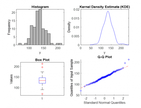
Figure 3. Histogram, kern density, box plot and QQ plot of the set data 1
Tables 3 and 4 provide a comparison of the proposed NLEVD with several life time distributions based on fit statistics such as AIC, BIC and log-likelihood the lower the better here. This is clear from the parameter estimates and standard errors, which present the NLEVD’s adaptable nature, which allows it to estimate data characteristics of different types. Due to these reasons, the application of the NLEVD to two real datasets is used to compare with other models, using histograms and probability plots. A comparison of two methods of the estimation of the parameters (SVM and MLE) reveal that the former is better than the latter in that it has higher prediction accuracy especially on and non-linear data the MLE is best suited for simple models. From the result above, SVM presented a lower AIC and BIC than both EB and ML indicating better model fit and estimation for the NLEVD. This goes a long way to show why the specification of the appropriate method of estimation should be determined by the type of data available as shown in Figure 3.
Table 3. The MLE estimates, -2 log-likelihood, AIC, BIC, and CAIC for data set I
|
Models |
MLE |
||||
|
-2L |
AIC |
BIC |
CAIC |
p-value |
|
|
Extension Exponential [24] |
557.8887 |
561.8887 |
567.1189 |
562.0111 |
0.0031 |
|
Gamma Lindley [25] |
556.3985 |
560.3985 |
565.6287 |
560.5209 |
0.0008 |
|
X Lindley [26] |
559.3096 |
561.3096 |
563.9247 |
561.35 |
0.0033 |
|
Zaghdoudi [27] |
537.8028 |
539.8028 |
542.4179 |
539.8432 |
0.0043 |
|
Exponential [28] |
595.4801 |
597.4801 |
600.0952 |
597.5205 |
0.0022 |
|
Lindley [29] |
558.606 |
560.606 |
563.2211 |
560.6464 |
0.0044 |
|
X gamma [30] |
539.132 |
541.132 |
543.7471 |
541.1724 |
0.0041 |
|
NLEED [31] |
458.4121 |
460.4121 |
467.6423 |
462.5345 |
0.0007 |
|
New Model (NLEVD) |
246.9134 |
252.9134 |
260.1234 |
254.5678 |
0.0005 |
Table 4. The SVM estimates, -2 log-likelihood, AIC, BIC, and CAIC for data set I
|
Models |
SVM |
|||
|
-2L |
AIC |
BIC |
CAIC |
|
|
Extension Exponential [24] |
432.8295 |
459.659 |
460.8916 |
451.1242 |
|
Gamma Lindley [25] |
426.8295 |
439.659 |
435.8916 |
431.1242 |
|
X Lindley [26] |
454.3239 |
412.6478 |
416.8029 |
426.958 |
|
Zaghdoudi [27] |
437.0757 |
438.1513 |
442.3064 |
442.4615 |
|
Exponential [28] |
447.6714 |
419.3428 |
423.4979 |
433.653 |
|
Lindley [29] |
426.8295 |
457.659 |
461.8141 |
451.9692 |
|
X gamma [30] |
459.6029 |
423.2059 |
427.361 |
437.516 |
|
NLEED [31] |
409.728 |
408.5655 |
409.7981 |
410.0307 |
|
New Model (NLEVD) |
202.2631 |
207.5261 |
206.7587 |
201.9913 |
8.1 Data set 2
Parameter the data set [2], they deal with an accelerated life test experiment on 59 conductors. The failure mechanism under study is electromigration, which is a process occurring within the conductors, and causing failure of microcircuits. The data contain the failure time in hour and there is no censoring in this data set. This data set is well known in the reliability engineering and survival analysis literature and therefore provides a useful framework for comparing the performance of statistical models in the context of failure time analysis. The second part of Table 5 represents the maximum likelihood estimation results, the AIC, BIC, CAIC and the p-values of different models that were fitted to this data.
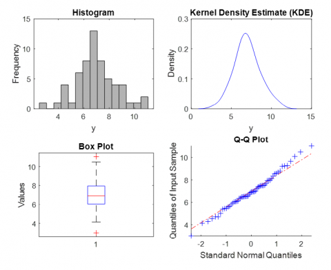
Tables 5 and 6 present the results of the NLEVD compared to other lifetime distributions based on AIC, BIC and log likelihood fit statistics, where lower values of all of these statistics are better fit. By using the parameter estimates and standard errors we observe how the NLEVD is able to fit many data characteristics. This is well demonstrated by the use of the NLEVD to two real databases in which it provides a much better fit than the models under analysis based on both histograms and probability plots. A fresh comparison between the parameter estimation techniques viz. the SVM and the MLE shows that SVM indeed gives better prediction accuracy over the MLE specially for non-linear data while is preferable for simple models. The findings also show that AIC and BIC are lower for SVM than for EB and ML, thereby showing that the own-letters NLEVD fits better with this algorithm. This shows that depending on the type of data the correct estimation technique should be used as shown in Figure 4.
Table 5. Fitting and prediction results derived from different models using the fault dataset, including those using MLE approaches [2]
|
Models |
MLE |
||||
|
-2L |
AIC |
BIC |
CAIC |
p-value |
|
|
Extension Exponential |
152.5082 |
156.5082 |
160.6632 |
156.7224 |
0.0021 |
|
Gamma Lindley |
137.1553 |
141.1553 |
145.3103 |
141.3695 |
0.0007 |
|
X Lindley |
162.4521 |
163.4521 |
166.5296 |
164.5222 |
0.0030 |
|
Zaghdoudi |
144.2481 |
145.2481 |
144.3256 |
146.3182 |
0.0033 |
|
Exponential |
195.4801 |
197.4801 |
190.0952 |
197.5205 |
0.0012 |
|
Lindley |
158.3527 |
159.3527 |
162.4302 |
160.4228 |
0.0034 |
|
X gamma |
154.5598 |
155.5598 |
158.6373 |
156.6299 |
0.0031 |
|
NLEED |
119.6421 |
123.6421 |
127.7971 |
123.8563 |
0.0006 |
|
New Model (NLEVD) |
114.64 |
120.23 |
127.67 |
122.89 |
0.0004 |
Table 6. Fitting and prediction results derived from different models using the fault dataset, including those using SVM approaches [2]
|
Models |
SVM |
|||
|
-2L |
AIC |
BIC |
CAIC |
|
|
Extension Exponential |
132.8295 |
159.659 |
160.8916 |
151.1242 |
|
Gamma Lindley |
126.8295 |
139.659 |
135.8916 |
131.1242 |
|
X Lindley |
154.3239 |
112.6478 |
116.8029 |
126.958 |
|
Zaghdoudi |
137.0757 |
138.1513 |
142.3064 |
142.4615 |
|
Exponential |
147.6714 |
119.3428 |
123.4979 |
133.653 |
|
Lindley |
126.8295 |
157.659 |
161.8141 |
151.9692 |
|
X gamma |
159.6029 |
123.2059 |
127.361 |
137.516 |
|
NLEED |
109.728 |
108.5655 |
109.7981 |
110.0307 |
|
New Model (NLEVD) |
102.2631 |
107.5261 |
106.7587 |
101.9913 |
Figure 4. Histogram, kern density, box plot and QQ plot of the set data 2
The discussion that follows underscores some of the advantages of the proposed NLEVD with a view to underlining its versatility and usefulness in statistical analysis. Further research should be directed in translating the NLEVD for multi-parameters data model for more flexibility of use, assessment of the NLEVD for other and various datasets under the different field such as health care, engineering and the environmental science, and applying more sophisticated and advanced artificial intelligence algorithms in the way of improving parameter estimation. Furthermore, enhancing program interfaces and studying theoretical features of this distribution including asymptotic properties and connections to other distributions, would enlarge its potential and improve mathematical background. By following these directions, the NLEVD can improve its recognition as a powerful tool in various domains applicable to survival analysis and reliability theory, and stimulate further theoretical and applied research in the field of statistics.
In this paper, we propose a new three-parameter continuous univariate distribution named NLEVD. We consider several prospective features of the NLEVD, including the CDF of the NLEVD, PDF of the NLEVD, survival function for the NLEVD, the hazard function for the NLEVD, and the quantile function for the NLEVD. Our study shows that the proposed distribution is applicable to many practical situations and has an inverted bathtub shaped instantaneous hazard rate. To estimate the parameters of the NLEVD, we employ two advanced methodologies: In this study, only two sets of predictors are assessed using two estimation techniques, namely the MLE method and SVM regression. The effectiveness of these estimation techniques is examined with the help of two real-life data sets and the general applicability, suitability and versatility of the proposed distribution is also discussed. The results of comparison show that the NLEVD is a more suitable model than one and two parameters such as New Extension Exponential, Gamma Lindley, Zeghdoudi, X Lindley, X gamma and Lindley. In addition, our findings reveal that when it comes to estimating the parameters of the proposed model, the ‘SVM’ method is superior to ‘MLE’ method thus showing that, harnessing electricity; machine learning can really help statistics. We expect that the to hold qualitative and quantitative duties in several disciplines, as a potential tool in fields such as survival analysis, probability theory and applied statistics will be useful for modeling complex data with different natures.
The authors are very grateful to the Duhok of Polytechnic University for providing access which allows for more accurate data collection and improved the quality of this work.
[1] Birnbaum, Z.W., Saunders, S.C. (1969). Estimation for a family of life distributions with applications to fatigue. Journal of Applied Probability, 6(2): 328-347. https://doi.org/10.2307/3212004
[2] Nelson, W., Doganoksoy, N. (2023). Statistical analysis of life or strength data from specimens of various sizes using the power-(log) normal model. In Recent Advances in Life-Testing and Reliability, pp. 377-408. https://doi.org/10.1201/9781003418313
[3] Shirawia, N., Kherd, A., Bamsaoud, S., Tashtoush, M., Jassar, A., Az-Zo’bi, E. (2024). Dejdumrong collocation approach and operational matrix for a class of second-order delay IVPs: Error analysis and applications. WSEAS Transactions on Mathematics, 23: 467-479. https://doi.org/10.37394/23206.2024.23.49
[4] Totaro, V., Gioia, A., Kuczera, G., Iacobellis, V. (2024). Modelling multidecadal variability in flood frequency using the two-component extreme value distribution. Stochastic Environmental Research and Risk Assessment, 38: 2157-2174. https://doi.org/10.1007/s00477-024-02673-8
[5] Yang, Y., Cui, J., Li, J. (2022). Reliability data analysis and lifetime prediction of aviation equipment based on logistic distribution. In 2022 15th International Symposium on Computational Intelligence and Design (ISCID), Hangzhou, China, pp. 260-263. https://doi.org/10.1109/ISCID56505.2022.00064
[6] Tahir, M.H., Cordeiro, G.M., Alzaatreh, A., Mansoor, M., Zubair, M. (2016). The logistic-X family of distributions and its applications. Communications in Statistics-Theory and Methods, 45(24): 7326-7349. https://doi.org/10.1080/03610926.2014.980516
[7] Hussain, A., Oraibi, Y., Mashikhin, Z., Jameel, A., Tashtoush, M., Az-Zo’bi, E.A. (2025). New software reliability growth model: Piratical swarm optimization -based parameter estimation in environments with uncertainty and dependent failures. Statistics, Optimization & Information Computing, 13(1): 209-221. https://doi.org/10.19139/soic-2310-5070-2109
[8] Hussain, A., Mahmood, K., Ibrahim, I., Jameel, A., Nawaz, S., Tashtoush, M. (2025). Parameters estimation of the Gompertz-Makeham process in non-homogeneous Poisson processes: Using modified maximum likelihood estimation and artificial intelligence methods. Mathematics and Statistics, 13(1): 1-11. http://doi.org/10.13189/ms.2025.130101
[9] Lemonte, A.J., Cordeiro, G.M., Moreno–Arenas, G. (2016). A new useful three-parameter extension of the exponential distribution, Statistics, 50(2): 312-337. https://doi.org/10.1080/02331888.2015.1095190
[10] Mansoor, M., Tahir, M.H., Cordeiro, G.M., Provost, S.B., Alzaatreh, A. (2019). The Marshall-Olkin logistic-exponential distribution. Communications in Statistics-Theory and Methods, 48(2): 220-234. https://doi.org/10.1080/03610926.2017.1414254
[11] Chaudhary, A.K., Kumar, V. (2020). Half logistic exponential extension distribution with properties and applications. International Journal of Recent Technology and Engineering (IJRTE), 8(3): 506-512. https://doi.org/10.22214/ijraset.2020.32565
[12] Lan, Y., Leemis, L.M. (2008). The logistic–exponential survival distribution. Naval Research Logistics (NRL), 55(3): 252-264. https://doi.org/10.1002/nav.20279
[13] Vapnik, V. (1995). The Nature of Statistical Learning Theory. Springer, New York. https://doi.org/10.1007/978-1-4757-3264-1
[14] Cortes, C., Vapnik, V. (1995). Support-vector networks. Machine Learning, 20: 273-297. https://doi.org/10.1007/BF00994018
[15] Boser, B.E., Guyon, I.M., Vapnik, V.N. (1992). A training algorithm for optimal margin classifier. In Proceedings 5th ACM Workshop on Computational Learning Theory, Pittsburgh, PA, pp. 144-152. https://doi.org/10.1145/130385.130401
[16] Liu, Y., Liu, B. (2024). A modified uncertain maximum likelihood estimation with applications in uncertain statistics. Communications in Statistics-Theory and Methods, 53(18): 6649-6670. https://doi.org/10.1080/03610926.2023.2248534
[17] Hussain, A.S., Sulaiman, M.S., Hussein, S.M., Az-Zo’bi, E.A., Tashtoush, M. (2025). Advanced parameter estimation for the Gompertz-Makeham process: A comparative study of MMLE, PSO, CS, and Bayesian methods. Statistics, Optimization & Information Computing, 13(6): 2316-2338. https://doi.org/10.19139/soic-2310-5070-2167
[18] Hussain, A., Pati, K., Atiyah, A., Tashtoush, M. (2025). Rate of occurrence estimation in geometric processes with maxwell distribution: A comparative study between artificial intelligence and classical methods. International Journal of Advances in Soft Computing and Its Applications, 17(1): 1-15. https://doi.org/10.15849/IJASCA.250330.01
[19] Banga, M., Bansal, A., Singh, A. (2019). Implementation of machine learning techniques in software reliability: A framework. In 2019 International Conference on Automation, Computational and Technology Management (ICACTM), London, UK, pp. 241-245. https://doi.org/10.1109/ICACTM.2019.8776830
[20] Adel, S.H., Fatah, K.S., Sulaiman, M.S. (2023). Estimating the rate of occurrence of extreme value process using classical and intelligent methods with application: Nonhomogeneous Poisson process with intelligent. Iraqi Journal of Science, 3054-3065. https://doi.org/10.24996/ijs.2023.64.6.33
[21] Cavanaugh, J.E., Neath, A.A. (2019). The Akaike information criterion: Background, derivation, properties, application, interpretation, and refinements. Wiley Interdisciplinary Reviews: Computational Statistics, 11(3): e1460. https://doi.org/10.1002/wics.1460
[22] Ibrahim, I., Taha, W., Dawi, M., Jameel, A., Tashtoush, M., Az-Zo’bi, E. (2024). Various closed-form solitonic wave solutions of conformable higher-dimensional Fokas model in fluids and plasma physics. Iraqi Journal for Computer Science and Mathematics, 5(3): 401-417. https://doi.org/10.52866/ijcsm.2024.05.03.027
[23] Az-Zo’bi, E., Kallekh, A., Rahman, R., Akinyemi, L., Bekir, A., Ahmad, H., Tashtoush, M., Mahariq, I. (2024). Novel topological, non-topological, and more solitons of the generalized cubic p-system describing isothermal flux. Optical and Quantum Electronics, 56(1): 1-16. https://doi.org/10.1007/s11082-023-05642-7
[24] Ragab, I.E., Alsadat, N., Balogun, O.S., Elgarhy, M. (2024). Unit extended exponential distribution with applications. Journal of Radiation Research and Applied Sciences, 17(4): 101118. https://doi.org/10.1016/j.jrras.2024.101118
[25] Chakroun, F., Abid, L., Elarbi, D., Masmoudi, A. (2024). Gamma–Lindley regression cure model for corporate credit default prediction. Expert Systems with Applications, 257: 125004. https://doi.org/10.1016/j.eswa.2024.125004
[26] Ghitany, M.E., Al-Mutairi, D.K., Balakrishnan, N., Al-Enezi, L.J. (2013). Power Lindley distribution and associated inference. Computational Statistics & Data Analysis, 64: 20-33. https://doi.org/10.1016/j.csda.2013.02.026
[27] Zaghdoudi, T., Tissaoui, K., Hakimi, A., Ben Amor, L. (2024). Dirty versus renewable energy consumption in China: A comparative analysis between conventional and non-conventional approaches. Annals of Operations Research, 334(1): 601-622. https://doi.org/10.1007/s10479-023-05181-0
[28] Wu, S. (2019). A failure process model with the exponential smoothing of intensity functions. European Journal of Operational Research, 275(2): 502-513. https://doi.org/10.1016/j.ejor.2018.11.045
[29] Barco, K.V.P., Mazucheli, J., Janeiro, V. (2017). The inverse power Lindley distribution. Communications in Statistics-Simulation and Computation, 46(8): 6308-6323. https://doi.org/10.1080/03610918.2016.1202274
[30] Yadav, A.S., Maiti, S.S., Saha, M. (2021). The inverse xgamma distribution: Statistical properties and different methods of estimation. Annals of Data Science, 8: 275-293. https://doi.org/10.1007/s40745-019-00211-w
[31] Meradji, A., Lazri, N., Zeghdoudi, H. (2024). Novel logistic exponential extension distribution: Properties and applications in applied sciences. Brazilian Applied Science Review, 8(2): e76168-e76168. https://doi.org/10.34115/basrv8n2-036