Chinniah Ramya![]() | SatheeshKumar Palanisamy*
| SatheeshKumar Palanisamy*![]() | Sghaier Guizani
| Sghaier Guizani![]()
© 2025 The authors. This article is published by IIETA and is licensed under the CC BY 4.0 license (http://creativecommons.org/licenses/by/4.0/).
OPEN ACCESS
Agriculture plays a vital role in food production and economic stability, but plant diseases can severely affect crop yields, leading to global losses. Efficient and accurate disease detection is essential for sustainable agriculture. In this study, a deep learning-based approach for plant disease detection using convolutional neural networks (CNNs) is proposed. The proposed model combines batch normalization, Adam optimizer with exponential learning rate, and ReLU activation function to improve learning efficiency and generalization. A dataset of 70,000 images is used for training and evaluation. The model successfully classifies plant leaves as healthy or diseased and identifies specific diseases with 99.4% accuracy. Performance metrics such as precision (96.77%) and recall (96%) further validate the robustness of the proposed system. The integration of advanced optimization techniques improves the convergence speed and classification accuracy compared to traditional methods, making the model well suited for real-world agricultural applications. The results of the study demonstrate the potential of AI-driven smart agricultural systems for early disease detection, enabling timely intervention and improving overall crop health.
Plant disease detection, smart agriculture, deep learning, batch normalization, convolutional neural network (CNN), image classification
Plant diseases can significantly impact crop yield and food production, leading to reduced agricultural productivity and global losses. In severe cases, plant diseases caused by pests can hinder plant development at various growth stages, affecting harvests. Over the years, numerous methods have been proposed for disease identification in plants. However, these methods often require specialized expertise, making them difficult for non-experts to implement effectively. Among various approaches, deep learning-based models have demonstrated significant promise in identifying plant diseases using leaf images. These models aid in diagnosing diseased plants by distinguishing them from healthy ones through digital analysis, benefiting small-scale farmers in low-income regions.
Despite their effectiveness, deep learning models face challenges such as overfitting, computational complexity, and handling large datasets. These issues can be addressed using Convolutional Neural Networks (CNNs), which optimize computational efficiency by reducing the number of layers. The incorporation of data augmentation techniques, such as image rotation and resizing, further enhances model performance and accuracy.
This paper proposes a plant disease detection system that comprises three key steps:
A neural network consists of multiple neurons organized in a layered structure, where adjacent layers are interconnected to enable intelligent learning. This network intelligence allows neurons to process user input and generate accurate outputs. In this study, a CNN is employed due to its efficiency in handling large datasets. The dataset used in this research comprises 70,000 images, making CNN a suitable choice for processing extensive agricultural data. Table 1 summarizes the diseases against various plants and datasets for analysis.
A. Pre-processing layer
Images are imported to the input layer. Before that, certain pre-processing operations are to be performed, like image resizing rotation, etc. CNN requires fewer pre-processing operations when it’s compared to other neural network models, which makes it more efficient.
B. Convolutional layer
The convolutional layer is responsible for condensing the input image by extracting features and producing a feature map. Convolutional layers have various parameters like input image size, kernel/filter size, depth, and stride. A non-linear activation function is required for the breaking of the simple linear combination of the input. ReLU activation function is being since it is widely regarded for activation convolutional outputs.
ReLU(a)=max(0,a)
Batch normalization comes under the normalization technique, which is done between the hidden layers of the neural network to increase the learning rates and skip the intermediate layers based on the knowledge obtained previously.
C. Pooling layer
Pooling increases the efficiency of the CNN model by preventing overfitting, thus reducing the dimensionality of the data thus leading to the reduction of calculations. Max pooling and average pooling are the most frequently used in the CNN model.
D. Fully connected classification layer
It takes the convoluted feature map and returns a column vector where each row indicated a class (the estimation of each class) In general, input images after pre-processing phase, the data flows into convolutional layers (the number of layers depends upon the choice of the designer), then to the next layer which is pooling layers which is responsible for feature extraction, and redundancy is reduced efficiently.
After that, the obtained features are combined and then labeled as a class. At last, the selected features are passed to the fully connected layer, and then estimation is provided.
Table 1. Vegetable and fruit leaves with diseases
|
Plant |
Disease |
Number of Images |
|
Grape |
Black Rot |
1913 |
|
Early Blight |
1988 |
|
|
Esca Measles |
1816 |
|
|
Healthy |
1987 |
|
|
Orange |
Citrus Greening |
1760 |
|
Bacterial Spot |
2016 |
|
|
Healthy |
2008 |
|
|
Potato |
Late Blight |
1888 |
|
Early Blight |
1920 |
|
|
Healthy |
1692 |
|
|
Coffee |
Bacterial Spot |
1722 |
|
Healthy |
2010 |
|
|
Cotton |
Black Rot |
1838 |
|
Cedar Cotton rust |
1728 |
|
|
Cotton Scab |
1939 |
|
|
Tea |
Healthy |
1781 |
|
Powdery Mildew |
2022 |
|
|
Tomato |
Bacterial Spot |
1736 |
|
Late Blight |
1824 |
|
|
Early Blight |
1774 |
|
|
Healthy |
1642 |
|
|
Leaf Mold |
1907 |
|
|
Septoria Leaf Spot |
1908 |
|
|
Spider Mites |
1826 |
|
|
Target Spot |
1683 |
|
|
Mosaic Virus |
1702 |
|
|
Leaf Curl |
1920 |
|
|
Sugarcane |
Northern Leaf Blight |
1926 |
|
Common Rust |
1851 |
|
|
Cercospora |
1822 |
|
|
Healthy |
1745 |
|
|
Strawberry |
Healthy |
1731 |
|
Leaf scorch |
1827 |
Conventional disease detection systems primarily rely on image analysis techniques that require prior domain knowledge to describe visual symptoms using parameters such as shape, color, and texture. Numerous deep learning-based plant disease identification models have been developed to overcome these limitations [1]. Among these, CNNs have demonstrated superior efficiency due to their ability to autonomously learn features from input images [2, 3]. However, CNN models typically consist of multiple layers, increasing parameter complexity and leading to overfitting during training. To mitigate this, transfer learning techniques have been deployed, where pre-trained CNN models on large datasets are fine-tuned on smaller datasets to enhance generalization [4].
2.1 CNN-based approaches in plant disease detection
CNN-based plant disease detection techniques utilize image classification methods, where features are extracted through multiple convolutional layers. Binary classification models typically categorize leaves into diseased-positive and diseased-negative classes, as demonstrated in studies focusing on Huanglongbing (HLB) disease classification [5]. Some models extend to multi-class classification using a two-stage approach: first identifying diseased versus healthy leaves, then classifying specific diseases in the second stage [6]. Alternatively, a single-phase multi-class classification model can differentiate between multiple diseases and healthy cases simultaneously [7].
Recent advancements have explored EfficientNetV2 [8] and U2-Net architectures, which improve classification accuracy while reducing computational costs. Additionally, segmentation techniques such as k-means clustering and U-Net are used to remove background data and isolate diseased regions before classification [9]. Sparse representation techniques further refine classification by analyzing color-based segmented portions. Ocular-attention deep neural networks have been employed to improve interpretability by highlighting crucial regions in the feature maps [10].
2.2 Object detection and optimization techniques
Region-based deep learning models, such as single-shot multi-box detectors (SSD) combined with Visual Geometry Group (VGG) networks, have been utilized for precise leaf disease detection [11]. Other studies incorporate multiple pre-trained deep learning models for enhanced classification accuracy [12]. Transfer learning has been successfully implemented to address overfitting, as seen in applications using AlexNet for cucumber and tomato disease detection [13], ResNet and DenseNet for apple and soybean leaf disease classification [14], and CNN-based models for peach leaf disease recognition [15].
2.3 IoT and smart agriculture integration
Low-power embedded systems with machine learning capabilities have enabled autonomous pest detection in fruit orchards using pheromone-based traps, with integrated energy harvesting ensuring continuous operation without farmer intervention [16]. An IoT-based deep learning framework, APDDCM-SHODL, enhances plant disease detection and crop management by employing DenseNet201 for feature extraction and a recurrent spiking neural network (RSNN) for classification, achieving 98.60% accuracy [17]. Similarly, an automated system integrating IoT, blockchain, and deep learning has improved pest detection in paddy cultivation, reaching 98.91% accuracy using VGG19 and ensemble classifiers [18].
Advanced AI-driven models have enhanced disease detection, forecasting, and control in crops such as potatoes by integrating image and climate data, achieving near-perfect accuracy [19]. CNN-based image recognition combined with unmanned aerial vehicles (UAVs) has further improved large-scale agricultural disease monitoring, highlighting the tradeoff between robustness and computational efficiency [20]. Edge intelligence and motion-static collaboration techniques, leveraging YOLO-FDAC and ant colony optimization, have been explored to enhance real-time crop disease detection using IoT-integrated image acquisition systems [21].
2.4 Optimization strategies for deep learning models
Most existing agricultural disease detection models rely on CNN architectures optimized using standard Adam or SGD optimizers. However, these approaches often suffer from slow convergence, unstable training dynamics, and suboptimal feature extraction due to inconsistent learning rates and lack of adaptive regularization [22]. While batch normalization has been utilized to improve feature learning, its synergy with learning rate scheduling remains underexplored. To address these challenges, this study proposes a novel power-exponential learning rate scheduler combined with batch normalization within the Adam optimizer. This technique enhances convergence speed, model stability, and generalization capabilities, making the model more robust for real-world agricultural disease classification. The proposed method facilitates automated pest detection and early disease identification in crops, enabling timely interventions to prevent yield loss and improve crop health.
2.5 Impact of proposed study in relevant to existing methodology
This study addresses several gaps in existing works, emphasizing its originality in the following ways:
Models that are developed using deep learning find their purpose in image processing and well as image reorganization domains. This paper takes the novelty of proposing a model which has been developed by applying the concepts of deep learning in the agricultural sector to produce results with improved efficiency when compared to the previously established models. The design flow of the proposed method is shown in Figure 1.
Figure 1. Design flow of the model proposed model
The design flow has been explained in detailed with their respective mathematical equations below.
Step 1: Image acquisition
The first step in the design flow is image acquisition where the images will be acquired from our Diseased leaf detection database. This database consists of over 70,000 images of different leaves with different sizes and resolutions.
i. Structure of the digital image
Digital images in general, are actually a combination of numerous matrices of numbers and each number being represented in the matrix is a representation of the brightness of a single pixel. In the case of traditional black-and-white images, there is a requirement for only one matrix. When it comes to color images, it is made up of three matrices that individually represent 3 color channels which are red, blue, and green. The matrices contain a range of values from 0 to 255.
Step 2: Image resizing and data augmentation
The images in the dataset are in different formats and also have different resolutions. Thus, all images are pre-processed before using them. The images are resized to 256×256 pixels. Several operations are performed on the images like rotation, resizing, etc.
The mathematical equation for rotation is shown below:
$x 2=\cos (\alpha) *(x 1-x 0)+\sin (\alpha) *(y 1-y 0)$ (1)
$y 2=-\sin (\alpha) *(x 1-x 0)+\cos (\alpha) *(y 1-y 0)$ (2)
where, $(x 1, y 1)$ are the original coordinated being rotated by an angle $(\alpha)$ around $(x 0, y 0)$ finally producing $(x 2, y 2)$.
The mathematical equation for resizing is as follows:
$\mathrm{w} 1=(a * r)^{\frac{1}{2}}$ (3)
$h 1=w1/r$ (4)
where, $w 1$ and $h 1$ denote the resized width and height of the image and r is the aspect ratio, which can be deduced as:
$r=w/h$ (5)
where, w and h denote the original width and height of the image.
Step 3: Feature extraction and classification
In image processing, convolution has been considered an efficient method for feature extraction since it effectively reduces the dimensions of the data thus providing a lesser redundant data set which can also be called a feature map.
3.1 Convolution
Kernel convolution is a concept widely applied across many simple and complex computer algorithms. A kernel is nothing but a small matrix consisting of numbers. Kernel convolution is a process where we take the kernel and transformation is done by passing it over the given image. Considering our input image to be i and our kernel to be k, rows and column index is represented by m and n respectively the process can be mathematically represented as the following
$G[m+n]=(i * k)[m, n]=\sum_j \sum_k k[j, k] i[m-j, n-k]$ (6)
By selecting a particular pixel and placing the filter over that particular pixel, multiplication by pairs is done by taking each and every value from the kernel with the corresponding values in the image. Last, performing a sum operation and then representing the result in its corresponding position in the output which is a feature map.
3.2 Padding
By performing convolution, the image tends to shrink every time the operation is performed. This makes the feasibility of the operation to be performed a limited number of times. If the threshold is crossed this might lead to the image getting disappeared completely. Thus, we lose the information contained in the image. To solve this problem, padding an image with an additional border is being done. The additional padding is usually filled with zeros. There are 2 types of convolutions whether padding is being used or not. If padding is done, then width of padding can be calculated using the following equation. Here, w is the width k is the kernel dimension. The equation is represented below
$\text{w}=\frac{k-1}{2}$ (7)
The dimensions of the output matrix when padding and stride is taken into account is represented below
$nout=1+\frac{nin+2w-k}{s}$ (8)
3.3 Activation function
In CNN, the purpose of an activated function is to calculate the weighted sum and add bias to it, and based on the result decision is made on whether to activate the particular neuron or not. Its main purpose is to add non-linearity to a neuron’s output. Rectified linear activation function, or ReLU, is a piecewise linear function that produces an output in response to an input. Positive input results in positive output, whereas negative input results in zero output.
ReLU(a)=max(0,a) (9)
3.4 Adam optimizer
The feature maps which are the output of the convolutional layer are the input to the pooling layer which reduces the dimension of the feature extracted earlier. The fully connected layer uses these redefined features for the classification of the input image into the categories defined by the user earlier.
Instead of a traditional Adam optimizer, Adam optimizer deployed with a power exponential learning rate is used for increasing the optimization rate in the CNN model since the adjustment with respect to the learning rate can be done according to the previous stages’ learning rate. This help in concision of learning rate in the minimum possible way leading to the stabilization of the parameters thus enhancing the effectiveness of the model.
The power- exponential learning rate adapts dynamically based on previous learning rates and gradients, improving convergence. Unlike step decay (which reduces the learning rate at fixed intervals) and cosine decay (which follows a sinusoidal pattern), the power-exponential scheduler dynamically adapts based on prior learning rates and gradient behavior. This allows smoother convergence and better stability across epochs. Empirical ablation studies comparing it to standard Adam and cosine decay schedulers will be presented in future work.
Pseudo Code 1: Adam optimizer deployed with power exponential learning rate
|
Algorithm: Adam optimizer deployed with a power-exponential learning rate, $\theta$: parameters, $m$, $v$: first and second moment estimates, $\beta_0$, $\beta_1$: exponential decay rates, |
|
Requirement: $\eta_1=0.1, \beta_0=0.9, \beta_1=0.999, \varepsilon=0.9999, Q=0.8$ |
|
Requirement: Initialize time step $\mathrm{t}_0$, parameter $\theta$, first/second-moment estimation $\widehat{m_{t 0}}, \widehat{v_{t 0}}$ while stopping criterion is not met do, Updating first/second moment: $m_{t 0} \leftarrow \beta_0 m_{t 0-1}+\left(1-\beta_0\right) g_t, v_{t 0} \leftarrow \beta_1 v_{t 0-1}+\left(1-\beta_1\right) g_t^2$ Moment correction: $\widehat{m_{t 0}} \leftarrow \frac{m_{t 0}}{1}-\beta_0^t, \widehat{v_{t 0}} \leftarrow \frac{v_{t 0}}{1}-\beta_1^t$ Power-exponential learning rate $\eta \leftarrow \eta_1 m^{-k}, m \leftarrow 1+\frac{t}{r^r} ; \eta(t) \leftarrow \eta_1\left[1+\frac{t}{r}\right]^{-k}$ Update parameters: $\theta_{t 0} \leftarrow \theta_{t 0-1}-\eta_1\left[1+\frac{t}{r}\right]^{-k} \frac{\widehat{m_{t 0}}}{\sqrt{\widehat{v_{t 0}}}+\varepsilon}$ |
|
Return optimized parameters $\theta$ |
3.5 Batch normalization
Batch normalization comes under the normalization technique, which is done between the hidden layers of the neural network to increase the learning rates and skip the intermediate layers based on the knowledge obtained previously. In general, a neuron without performing batch normalization is computed in the following manner.
$f(w, x)+b=\mathrm{i}$ (10)
$g(i)=\mathrm{A}$ (11)
where, f() is the linear transformation, w is the weight, b is the bias and g() is the activation function of the neuron.
If batch normalization is used, it can be computed in the following manner
$f(w, x)=i$ (12)
$(i)^n=\frac{i-m}{s} * \alpha+\beta$ (13)
$g(i)^n=A$ (14)
where, $i^n$ is the output of the batch normalization, m is the mean, s is the standard deviation of the neuron,
and are the batch normalization learning parameters. The comprehensive hyperparameter details include Batch size: 32, Epochs: 50, Architecture: 4-convolutional layers (kernel sizes: 3×3), ReLU activations, 2 MaxPooling layers, BatchNorm after each conv layer, 2 fully connected layers before output.Step 4: Output detection
Based on the input, features are being extracted and are being compared with the corresponding feature values that are stored correspondingly in feature dataset. Based on the analysis, it can be detected if the input image is healthy or diseased.
Pseudo Code 2: Pseudo code of proposed methodology
|
Considering input image to be i(x,y) |
|
i(x,y) undergoes image rotation $\begin{gathered}x 2=\cos (\alpha) *(x 1-x 0)+\sin (\alpha) *(y 1-y 0) \\ y 2=-\sin (\alpha) *(x 1-x 0)+\cos (\alpha) *(y 1-y 0)\end{gathered}$ i(x,y) undergoes resizing $\mathrm{w} 1=(a * r)^{\frac{1}{2}} ; h 1=w 1 / r$ where, $r=w / h$ i(x,y) undergoes convolution $G[m+n]=(i * k)[m, n]=\sum_j \sum_k k[j, k] i[m-j, n-k]$ Padding is done to i(x,y) $\begin{gathered}\mathrm{w}=\frac{k-1}{2} \\ \text { nout }=1+\frac{n i n+2 w-k}{s}\end{gathered}$ ReLU activation function and Adam optimizer is being used ReLU(a)=max(0,a) $\theta_{t 0} \leftarrow \theta_{t 0-1}-\eta_1\left[1+\frac{t}{r}\right]^{-k} \frac{\widehat{m_{t 0}}}{\sqrt{\widehat{v_{t 0}}}+\varepsilon}$ Batch normalization is being deployed to enhance the efficiency of the model being proposed $\begin{gathered}f(w, x)=\mathrm{i} \\ (i)^n=\frac{i-m}{s} * \alpha+\beta \\ g(i)^n=A\end{gathered}$ |
The considered dataset consists of 70,000 images of different sizes and resolutions. Pre-processing operations such as image resizing and rotation are performed on the input images to enhance the efficiency of the proposed CNN-based model. The dataset is divided into training and testing sets, ensuring a balanced distribution for effective learning and evaluation.
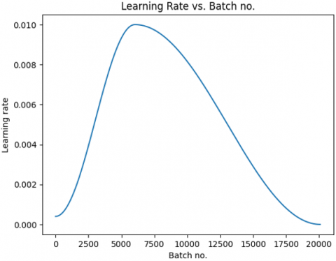
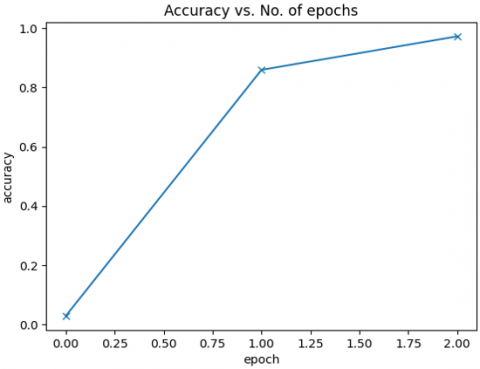
The proposed model is specifically trained on face-up leaf images, resulting in the highest accuracy when the input images are in the same orientation. Due to the use of batch normalization, the training process is accelerated by reducing the time required for additional calculations and parameter adjustments during backpropagation. Unlike traditional backpropagation, where the gradients may diminish as the number of layers increases-leading to challenges in weight initialization-batch normalization helps maintain stable gradient flow and optimizes weight updates. Figure 2 shows the improved learning rate of the model due to the deployment of batch normalization. To validate the generalization capability of the proposed model, 5-fold cross-validation was performed in addition to the standard train-test split. The dataset was divided into five equal subsets, and the model was trained and tested iteratively. The cross-validation results showed an average classification accuracy of 98.96%, with slight variations across folds, confirming the robustness and stability of the proposed architecture. To mitigate mild class imbalance observed in the dataset (e.g., Bacterial Spot: 2016, Leaf Mold: 1907), random oversampling was applied to underrepresented classes during batch formation. To enhance model robustness and generalization, data augmentation techniques such as random rotation (±25°), horizontal/vertical flipping (probability 0.5), brightness adjustment (±10%), and zooming (scale 0.9-1.1) were employed. These transformations were applied only during training, helping the model learn invariant features and reducing the risk of overfitting.
Additionally, batch normalization regulates the parameters entering the activation function, mitigating issues such as vanishing gradients and dead neurons in activation functions like ReLU. As a result, the proposed method demonstrates an improved learning rate and enhanced model generalization, contributing to higher classification accuracy in plant disease detection.
Figure 2. Improved learning rate of the model due to the deployment of batch normalization
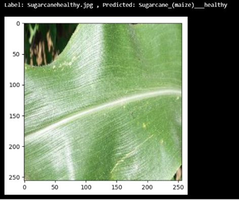
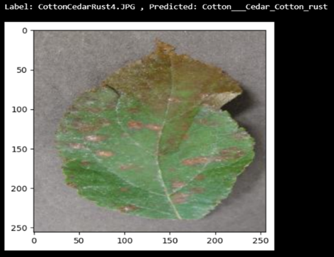
The proposed model successfully analyzes input leaf images and accurately predicts whether the leaf is healthy or diseased. If the leaf is diseased, the model further classifies it by identifying the specific disease affecting it. The detected model of healthy and diseased images is shown in Figures 3 and 4.
Figure 3. Detection by the model that input leaf is healthy
Figure 4. Detection by the model that input leaf is diseased
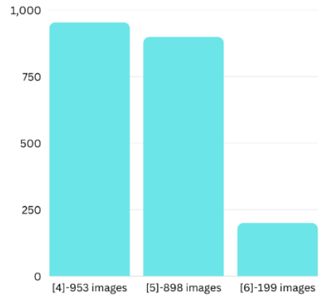
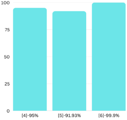
By incorporating batch normalization, the Adam optimizer with a power-exponential learning rate, and ReLU as the activation function, the proposed model achieves significantly higher accuracy compared to conventional models. While traditional approaches struggle with large datasets, such as the one used in this study, comprising 70,000 images, the proposed model demonstrates an estimated accuracy of 99.4% due to these enhancements. Figures 5-7 depict the size of the dataset and accuracy considered for the existing models with 70,000 images. Table 2 shows the performance comparative analysis of accuracy level with various datasets.
Figure 5. Depicts the size of the dataset considered for the existing models
Figure 6. Depicts the estimated accuracy of the existing models
Figure 7. Depicts the estimated accuracy of the proposed model with 70,000 images
Table 2. Performance comparison of accuracy level with various datasets
|
S. No. |
Model Type |
No. of Images in the Dataset |
Overall Accuracy (%) |
|
1. |
[4]-Existing |
953 |
95 |
|
2. |
[5]-Existing |
898 |
91.93 |
|
3. |
[6]-Existing |
199 |
99.9 |
|
4. |
[11]-Existing |
17,244 |
98.26 |
|
5. |
[17]-Existing |
16,225 |
97.50 |
|
6. |
[18]-Existing |
3,355 |
91.90 |
|
7. |
Proposed |
70,000 |
99.4 |
Performance metrics have been calculated for the proposed model. Common performance metrics parameters are accuracy, precision, recall, and mean F1 score, which is again based on precision and recall parameters.
Mean F1 score can be defined as
$\mathrm{F} 1=\frac{2 * P * R}{P+R}$ (15)
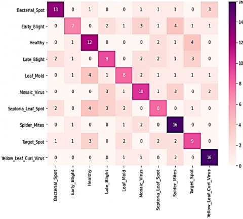
Performance metrics for the proposed model have been derived using the aforementioned formulae, and the confusion matrix has been shown in Figure 8. Table 3 shows the performance metrics analysis of various diseases.
Figure 8. Confusion matrix
Table 3. Performance Metrics analysis of various diseases
|
S. No. |
Disease |
Precision (%) |
Recall (%) |
F1-Score (%) |
|
1. |
Bacterial Spot |
72 |
65 |
68 |
|
2. |
Early Blight |
58 |
35 |
44 |
|
3. |
Healthy |
50 |
60 |
55 |
|
4. |
Late Blight |
50 |
45 |
47 |
|
5. |
Leaf Mold |
50 |
40 |
44 |
|
6. |
Mosaic Virus |
48 |
50 |
49 |
|
7. |
Septoria Leaf Spot |
44 |
40 |
42 |
|
8. |
Spider Mites |
52 |
80 |
63 |
|
9. |
Target Spot |
47 |
45 |
46 |
|
10. |
Yellow Leaf Curl Virus |
70 |
80 |
74 |
This study proposes an advanced deep learning-based plant disease detection system that effectively classifies and diagnoses plant diseases using a dataset of 70,000 images. By integrating batch normalization, the Adam optimizer with a power-exponential learning rate, and ReLU activation, the proposed model achieves superior performance, addressing common challenges such as overfitting and computational inefficiency. The system outperforms conventional models with an estimated accuracy of 99.4%, precision of 96.77%, and recall of 96%, demonstrating its effectiveness in large-scale agricultural disease classification. The results highlight the potential of AI-driven solutions in precision agriculture, enabling farmers to detect plant diseases early and take corrective actions to minimize yield losses. Future work can focus on expanding the model's applicability by incorporating real-time image processing techniques, Internet of Things (IoT) integration, and UAV-based monitoring for enhanced scalability and field deployment.
The authors would like to thank Tamil Nadu State Council for Science and Technology (TNSCST) for supporting this study (Project code: EEE-1383).
[1] Al-Shahari, E.A., Aldehim, G., Aljebreen, M., Alqurni, J. S., Salama, A.S., Abdelbagi, S. (2025). Internet of things assisted plant disease detection and crop management using deep learning for sustainable agriculture. IEEE Access, 13: 3512-3520. https://doi.org/10.1109/ACCESS.2024.3397619
[2] Rahman, W., Hossain, M.M., Hasan, M.M., Iqbal, M.S., Rahman, M.M., Hasan, K.F., Moni, M.A. (2024). Automated detection of harmful insects in agriculture: A smart framework leveraging IoT, machine learning, and blockchain. IEEE Transactions on Artificial Intelligence, 5(9): 4787-4798. https://doi.org/10.1109/TAI.2024.3394799
[3] Kaur, A., Randhawa, G.S., Abbas, F., Ali, M., Esau, T. J., Farooque, A.A., Singh, R. (2024). Artificial intelligence driven smart farming for accurate detection of potato diseases: A systematic review. IEEE Access, 12: 193902-193922. https://doi.org/10.1109/ACCESS.2024.3510456
[4] Nyakuri, J.P., Nkundineza, C., Gatera, O., Nkurikiyeyezu, K. (2024). State-of-the-art deep learning algorithms for internet of things-based detection of crop pests and diseases: A comprehensive review. IEEE Access, 12: 169824-169849. https://doi.org/10.1109/ACCESS.2024.3455244
[5] Li, X., Hou, B., Tang, H., Talpur, B.A., Zeeshan, Z., Bhatti, U.A., Liao, J., Liu, J., Alabdullah, B., Al Naimi, I.S. (2024). Abnormal crops image data acquisition strategy by exploiting edge intelligence and dynamic-static synergy in smart agriculture. IEEE Journal of Selected Topics in Applied Earth Observations and Remote Sensing, 17: 12538-12553. https://doi.org/10.1109/JSTARS.2024.3414306
[6] Boedeker, W., Watts, M., Clausing, P., Marquez, E. (2020). The global distribution of acute unintentional pesticide poisoning: Estimations based on a systematic review. BMC Public Health, 20: 1-19. https://doi.org/10.1186/s12889-020-09939-0
[7] Xu, Q., Cai, J.R., Zhang, W., Bai, J.W., Li, Z.Q., Tan, B., Sun, L. (2022). Detection of citrus Huanglongbing (HLB) based on the HLB-Induced leaf starch accumulation using a home-made computer vision system. Biosystems Engineering, 218: 163-174. https://doi.org/10.1016/j.biosystemseng.2022.04.018
[8] Adeem, G., ur Rehman, S., Ahmad, S. (2022). Classification of citrus canker and black spot diseases using a deep learning based approach. VFAST Transactions on Software Engineering, 10(2): 185-197. https://doi.org/10.21015/vtess.v15i3.976
[9] Farooq, M.S., Mehboob, A. (2023). Prediction of citrus diseases using machine learning and deep learning: Classifier, models SLR. arXiv preprint arXiv: 2306.01816. https://doi.org/10.48550/arXiv.2306.01816
[10] Sunil, C.K., Jaidhar, C.D. (2021). Cardamom plant disease detection approach using EfficientNetV2. IEEE Access, 10: 789-804. https://doi.org/10.1109/ACCESS.2021.3138920
[11] Tan, M., Le, Q. (2021). Efficientnetv2: Smaller models and faster training. In International Conference on Machine Learning, PMLR, pp. 10096-10106. https://doi.org/10.48550/arXiv.2104.00298
[12] Qin, X., Zhang, Z., Huang, C., Dehghan, M., Zaiane, O.R., Jagersand, M. (2020). U2-Net: Going deeper with nested U-structure for salient object detection. Pattern Recognition, 106: 107404. https://doi.org/10.1016/j.patcog.2020.107404
[13] Manso, G.L., Knidel, H., Krohling, R.A., Ventura, J.A. (2019). A smartphone application to detection and classification of coffee leaf miner and coffee leaf rust. arXiv preprint arXiv: 1904.00742. https://doi.org/10.48550/arXiv.1904.00742
[14] Neves, R.F., Wetterich, C.B., Sousa, E.P., Marcassa, L.G. (2023). Multiclass classifier based on deep learning for detection of citrus disease using fluorescence imaging spectroscopy. Laser Physics, 33(5): 055602. https://doi.org/10.1088/1555-6611/acc6bd
[15] Yeh, C.H., Lin, M.H., Chang, P.C., Kang, L.W. (2020). Enhanced visual attention-guided deep neural networks for image classification. IEEE Access, 8: 163447-163457. https://doi.org/10.1109/ACCESS.2020.3021729
[16] Li, W., Zheng, T., Yang, Z., Li, M., Sun, C., Yang, X. (2021). Classification and detection of insects from field images using deep learning for smart pest management: A systematic review. Ecological Informatics, 66: 101460. https://doi.org/10.1016/j.ecoinf.2021.101460
[17] Petchiammal, Kiruba, B., Murugan, Arjunan, P. (2023). Paddy doctor: A visual image dataset for automated paddy disease classification and benchmarking. In Proceedings of the 6th Joint International Conference on Data Science & Management of Data (10th ACM IKDD CODS and 28th COMAD), Mumbai, India, pp. 203-207. https://doi.org/10.1145/3570991.3570994
[18] Bhowmik, A., Sannigrahi, M., Chowdhury, D., Das, D. (2022). RiceCloud: A cloud integrated ensemble learning based rice leaf diseases prediction system. In 2022 IEEE 19th India Council International Conference (INDICON), Kochi, India, pp. 1-6. https://doi.org/10.1109/INDICON56171.2022.10039790
[19] Albanese, A., Nardello, M., Brunelli, D. (2021). Automated pest detection with DNN on the edge for precision agriculture. IEEE Journal on Emerging and Selected Topics in Circuits and Systems, 11(3): 458-467. https://doi.org/10.1109/JETCAS.2021.3101740
[20] Ahmad, I., Yang, Y., Yue, Y., Ye, C., Hassan, M., Cheng, X., Wu, Y., Zhang, Y. (2022). Deep learning based detector YOLOv5 for identifying insect pests. Applied Sciences, 12(19): 10167. https://doi.org/10.3390/app121910167
[21] Li, W., Zhu, T., Li, X., Dong, J., Liu, J. (2022). Recommending advanced deep learning models for efficient insect pest detection. Agriculture, 12(7): 1065. https://doi.org/10.3390/agriculture12071065
[22] Toscano-Miranda, R., Toro, M., Aguilar, J., Caro, M., Marulanda, A., Trebilcok, A. (2022). Artificial-Intelligence and sensing techniques for the management of insect pests and diseases in cotton: A systematic literature review. The Journal of Agricultural Science, 160(1-2): 16-31. https://doi.org/10.1017/S002185962200017X