Swathi Bonthala*![]() | Suhasini Ambalavanan
| Suhasini Ambalavanan![]() | Suvarchala Kakani
| Suvarchala Kakani![]()
© 2025 The authors. This article is published by IIETA and is licensed under the CC BY 4.0 license (http://creativecommons.org/licenses/by/4.0/).
OPEN ACCESS
Lung cancer is one of the deadliest diseases in the world affecting nearly five million individuals per year. The accurate detection and classification of lung cancer are crucial for proper treatment planning and increasing survival rates. In recent years, the convolutional neural network (CNN) emerged as an effective approach in lung tumor identification. However, the CNN face challenges such as computational complexity, increased training time, and limited generalization. This study proposed an optimized version of CNN named Spider Wasp optimization CNN (SWoCNN) for precise classification of lung cancer from computed tomography (CT) images. The presented SWoCNN incorporates the fast exploration capacity of spider wasp optimization (SWO) into the CNN algorithm for enhanced lung cancer classification. The developed strategy begins with the collection of lung CT images from both normal and cancer patients and the images are preprocessed to increase their quality. Consequently, an attention neural network (ANN) is developed for capturing and extracting the relevant features from the preprocessed images. Further, feature selection was done using the waterwheel plant algorithm (WPA), which selects the most informative features crucial for distinguishing the patterns of lung cancer. Finally, the proposed SWoCNN was trained using the selected features to classify lung cancer types. The SWO leverages its searching capacity to optimize and fine-tune the CNN hyperparameters to its optimal value, leading to improved classification, reduced computational time and fast CNN training. The proposed strategy was modeled and implemented in the Python platform and experimental results highlighted that the designed methodology achieved an average performance such as accuracy of 0.96407, precision of 0.96396, specificity of 0.96503, and false negative rate of 0.02963. Furthermore, a comparative assessment with existing models depicted that metrics such as accuracy, precision, recall, and specificity are enhanced by 1.23%, 1.24%, 1.19%, and 1.18%, respectively, depicting its reliability in classifying lung cancer.
lung cancer classification, CNN, spider wasp optimization, hyperparameter tuning
Lung cancer is one of the deadliest diseases that occur due to the abnormal growth of cells in the lungs, causing damage to healthy lung tissues [1]. The common cause of this cancer is tobacco usage and it accounts for nearly 80% of lung cancer deaths [2]. The study by the World Health Organization (WHO) on cancer reported that lung cancer has led to approximately 1.61 million deaths and it is more prominent among males than females. Early and precise identification of this disease is crucial for improving the patient's health and survival rate [3]. Currently, various imaging techniques including magnetic resonance imaging (MRI), Computed Tomography (CT), and X-ray are employed for lung cancer prediction [4]. Among these techniques, CT was widely used for lung cancer detection because of its effectiveness in capturing minute variations in the lung region [5]. Conventionally, the medical images are manually examined by healthcare professionals or radiotherapists to detect the presence of cancer [6]. However, this manual examination of cancer is time-consuming and it depends on the knowledge of the healthcare experts. Thus, researchers focused on developing an automatic framework leveraging advanced technologies such as artificial intelligence (AI), computer-aided processing, big data analysis, etc. [7]. In this automatic mechanism, the system was trained using the data containing both healthy and cancer features to understand the variations between them [8].
In recent times, AI approaches such as machine learning (ML) and deep learning (DL) have earned greater attention in image processing tasks. The AI-based models analyze the medical images and capture the features and hierarchical relations to detect the presence of lung cancer [9, 10]. Initially, the researchers utilized ML algorithms such as decision trees (DT), random forest classifier (RF), logistic regression, and support vector machine (SVM), for lung cancer detection [11, 12]. They process the medical images and train using either supervised or unsupervised learning strategies for classification tasks. The studies on ML models concluded that they offered automatic classification with increased accuracy than the manual process. Despite its increased performances, it faces challenges such as large computational demands, algorithmic bias, lack of adaptability, reduced accuracy in test cases, data dependency, etc. [13-15]. On the other hand, the DL models including deep neural network (DNN), CNN, and feed-forward neural network (FFNN) have shown promising results in image classification [16].
Among these neural networks, CNN is more suitable for medical image analysis because of its potential to capture features and relations within the images more effectively. Hence many researches are conducted on lung cancer classification using CNN models [17, 18]. The existing works developed techniques such as Fuzzy Particle Swarm Optimization with CNN [19], Deep CNN [20], 2-dimensional CNN [21], 3-dimensional CNN [22], autoencoder-based CNN [23], etc., for lung cancer detection. These strategies mainly focused on differentiating malignant and benign cells in the lung and achieved accuracy of around 86% to 95%. However, these frameworks face challenges such as computational complexity, minimum accuracy, instability, less generalization, and limited to binary classification. To address these issues, a novel optimized CNN was developed in this work for detecting and classifying lung cancer from CT images.
The major contributions of the presented framework are described below:
Identifying the cancerous nodules in lung CT images is crucial for diagnosing and classifying lung cancer. However, it is a complex and time-consuming process because of the varying size, texture, and shape of nodules. Asuntha and Srinivasan [19] presented an innovative solution for this problem using the DL model. This study designed a unique feature selector model by combining fuzzy function with particle swarm optimization (FPSO) and the selected features using FPSO to train CNN. This strategy was validated using the real-time CT image dataset gathered from Arthi Scan Hospital and the experimental outcomes demonstrated that the usage of FPSO reduces the computational complexity of the CNN. However, it faces complexity in validating the correctness and reliability of fuzzy variables, sets, and membership functions.
Faruqui et al. [20] designed a hybrid classifier model named LungNet having 22 layers of CNN. This study aims to identify and categorize lung cancer from CT scans using a deep CNN algorithm. This study used the lung cancer dataset containing 525,000 images. The results of the study illustrated that it achieved 94.81% accuracy and 3.35% false positive rate. However, the model's accuracy was reduced to 91.6% when classifying the different stages of lung cancer.
Biradar et al. [21] proposed an automatic lung cancer classifier using the DL algorithm. This study intends to detect lung cancer nodules with improved speed and accuracy. A 2-dimensional CNN was created to classify malignant and benign cells in the lungs and it was validated using the Kaggle CT scan dataset. The implementation results manifested that it achieved only 88.76% in detecting cancer nodules, which is not sufficient for real-world clinical scenarios.
Bangare et al. [22] developed a computer-aided approach to categorize lung cancer from CT images. Its primary concern is to increase the probability of survival rate of lung cancer-affected individuals through accurate and timely cancer detection. This work developed a 3-dimensional CNN with image pre-processor and segmentation to detect malignant and non-malignant cells in the lungs. The experimental results highlighted that this strategy achieved an accuracy of 86.42%, specificity of 86.72%, and recall of 86.11%. However, these performances are not sufficient for lung cancer classification in real healthcare institutions.
The previous studies [23-27] developed an integrated framework for classifying lung cancer. This strategy combined the efficiency of the autoencoder and CNN for efficient feature learning. In addition, an Adam optimizer was deployed for optimizing the entire classifier model, and a multispace image reconstruction algorithm was used to minimize the error. The results of the work suggested that it earned 95.79% accuracy in lung cancer nodule detection. Also, it obtained less processing time of 15 seconds (s). However, this methodology is data-dependent and cancer detection from low pixel images lowers its accuracy.
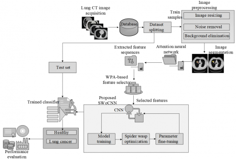
An optimized CNN was developed to classify lung cancer using lung CT images. The presented framework comprises five modules: image acquisition, image preprocessing, feature analysis, feature selection, and optimized model training and classification. In the data collection module, the CT images of healthy and lung cancer-affected individuals are gathered and imported into the system. The accumulated images are preprocessed following steps like noise filtering, image resizing, and background removal. Also, the U-Net algorithm was used for segmenting the region of interest (ROI) from the preprocessed images. In the feature extraction module, ANN was designed to capture the relevant attributes from the segmented images, which reduces the dimensionality of the data and improves training speed. Consequently, the WPA-based feature selector was modeled to select the most informative and highly correlative features from the extracted feature sets, enabling the classifier to concentrate on major features for tumor classification. Finally, an optimized CNN was developed by integrating the efficiency of SWO into it. The SWO continuously refines and optimizes the hyperparameters of CNN, enabling it /to adapt to evolving changes and enhancing its learning capacity. The architecture of the developed lung cancer classifier model is displayed in Figure 1.
Figure 1. Architecture of SWoCNN for lung cancer classification
3.1 Image acquisition
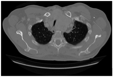
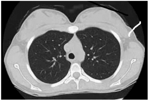
The first stage of the developed framework is the lung CT image acquisition from both healthy and cancer-affected persons as shown in Figure 2. The gathered images are labeled to train the classifier to recognize the patterns of lung cancer. The presented study used the publicly available Lung CT scan database from Kaggle site [27].
(a)
(b)
Figure 2. Dataset images of different classes: (a) Lung cancer; (b) Normal
3.2 Image preprocessing
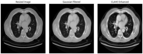
Image preprocessing defines the data preparation phase, where the system converts the raw CT images into an appropriate format for further processing. This stage follows a sequence of processes such as noise filtering, image resizing, and contrast enhancement or background elimination. In the noise filtering step, a Gaussian filter was applied to the images to eliminate the noise or unwanted random variations within each image. The Gaussian filter removes the noise attributes and replaces them with the average value of nearby or surrounding attributes, which is estimated by Gaussian distribution. The mathematical formulation of the Gaussian filter is expressed in Eq. (1):
$G s(m, n)=C_{i m}(m, n) \times \frac{1}{2 \pi \partial^2} e^{-\frac{m^2+n^2}{2 \partial^2}}$ (1)
where, Gs(m, n) represents the Gaussian filter, Cim(m, n) denotes the input CT image, (m, n) indicates the kernel coordinates, and ∂ refers to the standard deviation. Consequently, the filtered images are resized into a common size to boost the dataset consistency. Finally, background removal was done to discard the unwanted regions from the CT images. This process is done using image thresholding. This step helps the system to focus on useful regions in the images. In addition, data augmentation was performed to reduce the risk of overfitting. This step creates new training samples by performing steps like rotation, random translation, scaling, image mixing, etc. Figure 3 displays the preprocessed images.
Figure 3. Preprocessed images
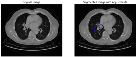
Further, image segmentation was done using the U-Net algorithm to isolate ROI from the preprocessed images [28]. This technique has the potential to segment the regions with training using less data. It consists of three main elements namely: encoder, bottleneck, and decoder. The encoder component down-samples the preprocessed images through convolution and pooling operations and maps the regions within each image. The bottleneck is placed between encoder and decoder and it maps the most informative regions while retaining spatial information. The encoder performs upsampling and reconstructs the image from the feature representation. The reconstructed image is the segmentation output. Figure 4 displays the segmentation outcomes.
Figure 4. Segmentation images
3.3 Feature extraction
An attention model is a kind of DL approach, which tends to concentrate on significant parts of the input data. In the proposed work, it was used to capture the relevant features from the segmented results. Feature extraction is one of the crucial steps in cancer classification, which aims to minimize the data dimension and assists the classifier in quickly learning the feature representations [29]. The architecture of ANN is similar to the structure of the encoder-decoder and finds the relevant features through the calculation of attention weights. It includes three main components namely: encoder, attention, and decoder. The encoder accepts the segmented images as input and generates hidden states (features present in the segmented images). The attention module determines the relevance between the encoder’s hidden state and the target hidden state and produces similarity scores as outcomes, which are mathematically expressed in Eq. (2):
$S w_{x t}^y=\omega\left(\tanh \left(w_e h_{x t}^y+b_{w e}\right)\right)+\beta$ (2)
where, $S w_{x t}^y$ represents the similarity score, ω denotes associated with ANN, tanh defines the activation function, $h_{x t}^y$ indicates the hidden state generated by the encoder, bwe denotes the bias vector associated with the attention component, we represent the weight vector of the attention module, and β indicates the bias vector of ANN. The resultant of the attention component is converted into attention weights using a Softmax function, as defined in Eq. (3):
$A w_t={soft} \max \left(S w_{x t}^y\right)$ (3)
where, Awt denotes the attention weights, which represents the relevance of the extracted feature for lung cancer categorization. These weights are applied to the encoder's hidden state and all the relevant information is extracted based on their importance through a weighted sum function, as represented in Eq. (4):
$W_{s t}=\sum_{t=1}^{T_m} A w_t h_{x t}^y$ (4)
where, Wst denotes the weighted sum and Ts indicates the maximum iteration. The decoder component receives the weighted sum and transforms it into a feature vector. This extracted feature vector contains all important information related to lung cancer classification.
3.4 Feature selection
Feature selection represents the process of selecting the most relevant attributes while eliminating the irrelevant ones. This step aims to enhance interpretability, reduce complexity, and increase accuracy. In the developed work, a novel feature selector was modeled using the meta-heuristic optimization algorithm named “Waterwheel plant algorithm [30].” The WPA is a bio-inspired approach modeled based on the natural characteristics of waterwheel plants to solve complex optimization problems. This algorithm is mathematically designed following the hunting expedition behavior of waterwheel plants. They use search agents to find the prey. Here, the concept of this algorithm is applied to select the most relevant and highly informative features for classifier training. The feature selection process begins with the initialization of extracted feature sets in the search space. In WPA, the extracted feature sets by ANN are expressed as a matrix using Eq. (5) and each feature is initialized in the search space using Eq. (6):
$F_e=\left[\begin{array}{l}F_{e l} \\ \vdots \\ F_{e i} \\ \vdots \\ F_{e Q}\end{array}\right]_{Q \times R}=\left[\begin{array}{cccc}f_{e(1,1)} & \ldots & f_{e(1, j)} & \dots & f_{e(1, R)} \\ \vdots & \ddots& \vdots & \ddots & \vdots \\ f_{e(i, 1)} & \ldots & f_{e(i, j)} & \ldots & f_{e(i, R)} \\ \vdots & \ddots & \vdots & \ddots & \vdots \\ f_{e(Q, 1)} & \ldots & f_{e(Q, j)} & \ldots & f_{e(Q, R)}\end{array} \right]$ (5)
$\begin{gathered}f_{e(i, j)}=L_{b j}+\kappa_{i, j} \cdot\left(U_{b j}-L_{b j}\right) \\ i=1,2,3, \ldots \ldots, Q, j=1,2,3, \ldots ., R\end{gathered}$ (6)
where, Fe indicates the extracted feature sets, Fei denotes the ith feature (candidate solution), fe(i,j) represents the jth problem variable, κi,j represents a random number (0, 1), Ubj and Lbj refers to the upper bound and lower bound. Further, the fitness value was determined for each feature based on their relevance to the tumor classification task, which is defined in Eq. (7):
$\gamma_v=\gamma_v\left[\begin{array}{l}F_{e 1} \\ \vdots \\ F_{e i} \\ \vdots \\ F_{e Q}\end{array}\right]_{Q \times R}$ (7)
The candidate solution with a high fitness value indicates the best or optimal solution and the solution with the lowest value denotes the worst. After fitness evaluation, the next step is exploration, where the system explores the search space and updates its initial values. This exploration helps to find the optimal solution and mitigates the possibility of local optima. The exploration phase of WPA is modeled using Eqs. (8) and (9):
$\vec{A}=\vec{d} \cdot\left(f_e(t)+2 \rho\right)$ (8)
$f_e(t+1)=f_e(t)+\vec{A} \cdot\left(2 \rho+\vec{d}_1\right)$ (9)
where, $\vec{A}$ denotes the direction of moving in the search space, fe(t+1) indicates the updated solution, fe(t) defines the current solution, $\overrightarrow{d_1} \vec{d}$ refers to the random vector, and $\rho$ represents the optimization factor. Consequently, the system exploits the current solutions to estimate the optimal features. This exploitation phase follows the hunting and feeding characteristics of WPA and it is formulated in Eqs. (10) and (11):
$\overrightarrow{A^{\prime}}=\vec{d}_2 \cdot\left(\rho \cdot f_e^{\prime}(t)+\vec{d}_3 f_e(t)\right)$ (10)
$f_e(t+1)=f_e(t)+\rho \overrightarrow{A^{\prime}.}$ (11)
where, $\overrightarrow{A^{\prime}}$ denotes the direction of exploitation, $\vec{d}_2$ and $\vec{d}_3$ indicates the random vector. Further, fitness value was determined for the updated solutions. Then, the feature with a fitness value greater than 0.5 is selected and this process continuous until reaching maximum iteration or maximum convergence rate. The selected features are fed into the classifier for training.
3.5 Optimized CNN for lung cancer classification
A meta-heuristic optimizer-based CNN was developed to accurately identify and categorize lung cancer by processing the CT images [31]. The developed algorithm incorporates the optimization and exploration characteristics of SWO into CNN, enabling the system to adapt to the evolving variations in the image features and to train the model with optimal values. The CNN is a popular DL model used for performing tasks such as object detection, speech recognition, video labeling, image classification, facial recognition, etc. It consists of five important layers namely: input, convolutional, pooling, and fully-connected (FC) layers. The input layer accepts the selected feature sets from the WPA module as classifier input and transforms them into a suitable format for feature learning. The convolutional layer is the building block of CNN, which is responsible for understanding the patterns within each image. It applies a sequence of kernel filters on the input data and creates a feature map, which represents the patterns influencing healthy and lung cancer-affected images. The feature map is mathematically expressed in Eq. (12):
$F_{m a p}(p, q)=\sum_{i=0}^{x-1} \sum_{j=0}^{y-1} S_f(x, y) * K(p-x, q-y)$ (12)
where, Fmap(p, q) indicates the feature map at the position (p, q), and K(p-x, q-y) represents the kernel filter applied at the location (p-x, q-y). Each convolutional layer is followed by a Rectified Linear Unit (ReLU) activation function to introduce non-linearity in the system. After each convolution+ReLU combination, a pooling layer was placed to reduce the spatial dimension, while retaining the significant information. This layer aims to minimize the memory and helps prevent overfitting by performing pooling operations. The pooling operation defines the process of sliding a 2-D filter over each channel of the feature map. In the designed CNN, a max pooling layer was used, which chooses the maximum element from the feature map covered by the 2-D filter. After multiple convolutional and pooling layers, the resultant feature map was flattened into a one-dimensional vector. This learned feature vector contains the patterns and relations between them, enabling them to categorize the lung cancer classes. The FC layer accepts this feature and computes the lung cancer classification through a Softmax function. The Softmax function returns the possibility of the input image belonging to the class, as represented in Eqs. (13) and (14):
$P_{v l}\left(C_{i m}\right)=\operatorname{Soft} \max \left(W_{f c} * f_{l e}\right)+b^{\prime}$ (13)
$C_{c l}= \begin{cases} { if }\left(0>P_{v l} \leq 0.2\right), & { normal } \\ { if }\left(P_{v l} \geq 0.3\right), & S C C\end{cases}$ (14)
where, Pvl indicates the probability value, Ccl denotes the classification function, Wfc defines the weight matrix of the FC layer, fle represents the flattened feature vector, and b' refers to the bias vector of the FC layer. Consequently, the loss or error was determined to estimate the efficiency of the classifier and it is formulated in Eq. (15):
Loss $=\frac{1}{S} \sum_{i=1}^S \sum_{j=1}^C Y_i^j \cdot \log \left(Y_i^{\prime j}\right)$ (15)
where, $Y_i^j$ denotes the ground truth outcome, S refers to the number of training samples, C indicates the number of classes, and ${Y^{\prime}}_i^j$ represents the predicted class. Reducing this loss is significant for improving classification accuracy. Also, the CNN's performance depends on the value of its hyperparameters such as several filters, kernel size, hidden layer, learning rate, batch size, weights, and bias vectors. To optimally select the values of these parameters, the SWO was integrated into CNN. The SWO is a meta-heuristic optimization algorithm developed based on the searching, hunting, mating, and nesting characteristics of female wasps [32]. The female wasps usually do these processes by depositing solitary egg within each spider’s abdomen. In the beginning stage of optimization, the female wasps explore their surroundings for finding suitable spiders. Then, they immobilize and pull them to make nests. After identifying appropriate nests and finding prey, they intend to drag the prey into nests. Unlike conventional optimization models such as genetic algorithm (GA), particle swarm optimization (PSO), grey wolf optimization (GWO), etc., the SWO dynamically switches between exploration and exploitation phases, leading to faster convergence and prevents premature convergence. In addition, the SWO model is more robust and efficient in optimizing the complex and high-dimensional spaces. Moreover, it offers diversified search options, which avoids the local optima. Since the SWO was used for selecting the optimal values in the search range, only the hunting phase is used in the designed model. The mating and nesting phases are not considered as they don’t directly relate with parameter update task, they are intended to reproduction and settlement of wasps in the biological systems The proposed optimization involves four phases: (i) initialization, (ii) fitness evaluation, (iii) searching phase, and (iv) parameter selection and termination.
i. Initialization
The SWO algorithm commences with the initialization of the female wasps. Each female wasp represents the CNN parameter set and it is initialized with a random value in the search space. In the context of CNN parameter tuning, female wasp defines the hyperparameter population, and prey denotes their optimal value The wasp population and the random initialization process are defined in Eqs. (16) and (17):
$\operatorname{Pr}=\left[\begin{array}{cccc}\operatorname{Pr}_{(1,1)} & \operatorname{Pr}_{(1,2)} & \ldots & \operatorname{Pr}_{(1, d)} \\ \operatorname{Pr}_{(2,1)} & \operatorname{Pr}_{(2,2)} & \ldots & \operatorname{Pr}_{(2, d)} \\ \vdots & \vdots & \vdots & \vdots \\ \operatorname{Pr}_{(c, 1)} & \operatorname{Pr}_{(c, 2)} & \ldots & \operatorname{Pr}_{(c, d)}\end{array}\right]$ (16)
$\overrightarrow{\operatorname{Pr}}_t=\vec{L}_u+\vec{r}\left(\vec{K}-\vec{L}_u\right)$ (17)
where, Pr indicates the parameter population, $\vec{L}_u$ $\vec{K}$ denotes the lower and upper bound of the search space and $\vec{r}$ represents the random initialization vector.
ii. Fitness evaluation
For each parameter set, fitness was calculated based on the predefined objective function. The objective function of the SWO is to reduce the loss incurred by CNN, and it is formulated in Eq. (18):
$O b j_{f u n}=\min \left(\frac{1}{S} \sum_{i=1}^S \sum_{j=1}^C Y_i^j \cdot \log \left(Y_i^{\prime j}\right)\right)$ (18)
The parameter set with high fitness indicates the optimal solution and vice versa. Then, the best candidate solution was estimated by sorting them as per their fitness value.
iii. Searching phase
This phase follows how female wasps search for the most suitable spiders for feeding their offspring. They use a constant step for searching for prey by randomly looking into the search space. Similarly, in the developed work, they look for the optimal value for the parameter set in the search range. In this searching phase, the values of the parameter set will be updated in two ways. The random exploration of search space and parameter update is formulated in Eq. (19):
${Pr}(t+1)={Pr}(t)+f .\left({Pr}_a(t)-{Pr}_b(t)\right)$ (19)
where, Pr(t) denotes the current parameter set, Pr(t+1) denotes the updated parameter set, ϕ represents the constant motion, a and b indicates two randomly selected indices to choose the exploration direction. In some instances, the optimization process drops and selects the local optima. To prevent this, the SWO algorithm explores the surrounding search space with a small step size, as expressed in Eq. (20):
${Pr}(t+1)={Pr}(t)+\phi \cdot \vec{L}_u+\vec{r}\left(\vec{K}-\vec{L}_u\right)$ (20)
where, $\vec{r}$ defines the random vector [0, 1]. In searching phase, the updated hyperparameters in the search space are determined using Eq. (21):
${Pr}(t+1)=\left\{\begin{array}{l}{Pr}(t)+f \cdot\left({Pr}_a(t)-{Pr}_b(t)\right) ; \text { if } c<g \\ {Pr}(t)+\phi \cdot \vec{L}_u+\vec{r}\left(\vec{K}-\vec{L}_u\right) ; { otherwise }\end{array}\right.$ (21)
where, χ and γ defines the random number ranging [0, 1], representing the probability of obtaining local optima in the searching phase.
$\begin{gathered}{Pr}(t+1)={Pr}(t) +G \times\left|2 \times r_e \times P r_a(t)-P r_b(t)\right|\end{gathered}$ (22)
where, G denotes the deviation between the current solution and the best solution, and re indicates the randomness in escaping in range [0, 1]. The formula for calculating G is expressed in Eq. (23):
$G=r_e \times\left(2-2 \times\left(\frac{t}{T_m}\right)\right)$ (23)
where, t indicates the current iteration, and Tm denotes the maximum iteration. This stage is the beginning of the exploitation stage in SWO approach.
v. Hunting phase
This phase follows how the female wasps move towards the region where the best spider (prey) can be found. The hyperparameter enters this stage only when its fitness is less than 0.3 (near optimal) and they are updated by exploiting locally. Instead of searching randomly, the algorithm adjusts current solutions by shifting them closer to the high-quality solutions, as formulated in Eq. (24):
$\begin{gathered}{Pr}(t+1)={Pr}(t)^{\prime} +\cos (2 p l) \times\left({Pr}(t)^{\prime}-{Pr}(t)\right)\end{gathered}$ (24)
where, Pr(t)' defines the best available solution. After updating hyperparameters, the fitness value was determined for them for selection purpose.
vi. Parameter selection and termination
If the fitness of the updated sequence is greater than the old fitness, the updated sequence was selected for modeling CNN. If the new fitness is less than the old fitness, no changes in CNN design the parameter selection is formulated in Eq. (25):
${Pr}= \begin{cases}{ if }\left(f_t^*<f_t\right) ,\ {Pr}(t+1) \\ { else } ,\ {Pr}(t)\end{cases}$ (25)
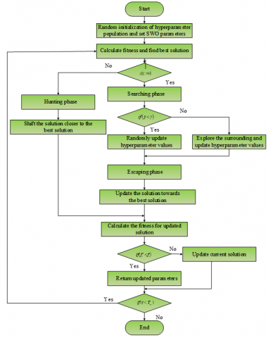
where, $f_t^*$ denotes the fitness of the updated hyperparameter, and ft indicates the fitness of the current solution. This process continues until it reaches maximum iteration. Algorithm 1 presents the working of the developed classifier in pseudocode format. Figure 5 presents the flowchart of the SWO algorithm for CNN parameter update.
Figure 5. The flowchart of the SWO algorithm for CNN parameter update
|
Algorithm: SWO-CNN |
|||
|
Input: Maximum iteration Tm, learning rate, kernel size, hidden layer, batch size, weights and bias vector, CT images; |
|||
|
Output: Lung cancer classification; |
|||
|
Start { |
|||
|
Design CNN with initial parameters (input, convolutional, pooling, and FC layers); |
|||
|
Train the model using selected features using WPA; |
|||
|
Estimate class probability; |
|||
|
Perform classification using Eq. (14); |
|||
|
Parameter optimization: |
|||
|
Define and initialize SWO parameters like population size c and decision variable d; |
|||
|
|
Initialize the initial value of the parameter set Pr; |
||
|
|
Randomly initialize parameter population pr using Eq. (17) |
||
|
|
Fitness evaluation: |
||
|
|
$O b j_{{fun }} \rightarrow \min (loss )$ |
||
|
|
for t=1: Tm |
||
|
|
|
Searching Phase: |
|
|
|
|
if(x<y) |
|
|
|
|
Update parameter set using Eq. (19); |
|
|
|
Else Update parameter set Pr using Eq. (20); |
||
|
|
|
End if; |
|
|
|
|
|
Escaping stage: |
|
|
Update the parameters towards the best solution using Eq. (21); |
||
|
|
|
Hunting Phase: |
|
|
|
|
if (ft<0.7) |
|
|
|
Update the parameter using Eq. (22); |
||
|
else |
|||
|
Exist; // the parameter set will not be updated in this phase |
|||
|
End if; |
|||
|
Determine fitness $f_t^*$ for the updated parameter set Pr(t+1); |
|||
|
if $\left(f_t^*<f_t\right)$ |
|||
|
Return Pr(t+1); |
|||
|
else |
|||
|
Return Pr(t); |
|||
|
t++; |
|||
|
end for; |
|||
|
Return optimal parameter value; |
|||
|
} End |
|||
The developed classifier was modeled and executed in Python software version 3.12.6 running on Jupyter Notebook 7.12, and supported by a Dell 11th Generation processor with 8GB RAM. The presented framework was trained and tested using the publicly available “Lung cancer CT scan dataset” from the Kaggle site.
4.1 Performance metrics
The definition and formula of parameters used for estimating the performance of the developed classifier in lung cancer categorization are defined below.
Accuracy: Accuracy defines the classifier’s effectiveness in categorizing both healthy and lung cancer and it quantifies the proportion of truly classified cases to the total instances. It measures the correctness of the system in classifying both normal and lung cancer images present in the dataset. It is represented in Eq. (26):
Accuracy $=\frac{t_p+t_n}{t_p+t_n+f_p+f_n}$ (26)
where, tp, tn, fp and fn represent TP, TN, FP, and FN, respectively.
Precision: Precision measures the classifier’s efficiency in identifying true positive cases to the total true instances, and it is formulated in Eq. (27). This metric quantifies the effectiveness of the model in classifying lung cancer among the true samples (real normal and lung cancer samples).
Precision $=\frac{t_p}{t_p+t_n}$ (27)
Sensitivity/recall: Recall determines the system’s proficiency to detect all relevant instances and it defines the fraction of real positive cases to the total positive cases, as defined in Eq. (28):
Recall $=\frac{t_p}{t_p+f_p}$ (28)
F-measure: F1-score denotes the harmonic mean of sensitivity and precision. It determines the balanced performance of the classifier in categorizing lung cancer, as formulated in Eq. (29). This parameter enables to determine the efficiency of the model in classifying normal and lung cancer images considering the false positive and negatives.
$F 1-score =2 \times\left(\frac{{ sensitivity }\ *\ { precision }}{ { sensitivity }\ +\ { precision }}\right)$ (29)
Specificity: Specificity measures the model's effectiveness in detecting and classifying normal (true negative) instances. It is represented mathematically in Eq. (30):
Specificity $=\frac{t_n}{t_n+f_p}$ (30)
False positive rate: FPR represents the ratio of actual negative cases that the system incorrectly categorizes as positive, as formulated in Eq. (31). It determines the incorrect lung cancer classification made by the system.
$F P R=\frac{f_p}{t_n+f_p}$ (31)
False negative rate: FNR denotes the ratio of real positive cases incorrectly categorized as negative by the system. It is expressed in Eq. (32):
$F N R=\frac{f_n}{t_p+f_n}$ (32)
Execution time:
The execution time determines the overall time consumed by the designed model for performing lung cancer identification and categorization. This measures the overall computational efficiency of the model in performing lung cancer classification.
The investigation of these parameters allows us to estimate how the classifier performs lung cancer classification.
4.2 Train and test phases
The presented framework was intensively trained with the Lung cancer CT scan dataset. Initially, the input dataset was split into the ratios of 80:20 for the train and test phases. The training phase begins with the initialization of CNN hyperparameters with initial value. The activation function of the CNN was ReLU, and the metrics like number of filters, kernel size, hidden layer range, learning rat, etc., are optimized by the SWO algorithm over the epoch (Table 1).
Table 1. The hyperparameter and its optimized value
|
Hyperparameter |
Range |
Optimized Value |
|
Number of filters for convolutional layer 1 |
[16, 32, 64, 96] |
64 |
|
Kernel size for convolutional layer 1 |
[3, 4, 5] |
3 |
|
Number of filters for convolutional layer 2 |
[48, 64, 96, 128] |
96 |
|
Kernel size for convolutional layer 2 |
[3, 4, 5] |
3 |
|
Number of filters for convolutional layer 3 |
[64, 96, 128] |
128 |
|
Kernel size for convolutional layer 3 |
[3, 4, 5] |
3 |
|
Batch size |
[5, 10, 20] |
20 |
|
Epoch |
[50, 100, 200] |
200 |
|
Hidden Layer (HL) 1 |
[75, 100, 125] |
100 |
|
HL 2 |
[75, 100, 125] |
125 |
|
Learning rate |
[0.001, 0.01, 0.1, 0.2] |
0.01 |
|
Activation |
- |
ReLU |
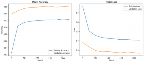
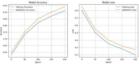
The outcomes during training and testing are determined using accuracy and loss metrics. Accuracy quantifies the classifier's efficiency in learning the hierarchical feature representations and its generalization capacity against real-world data. On the other hand, the loss measures the error made by the model during the training and test. Higher accuracy suggests that the model correctly classifies the lung cancer instances, while high loss indicates the model's inefficiency in categorizing the lung tumor cases.
The analysis of accuracy and loss in train and test phases is presented in Figure 6. The improvement of accuracy over the epoch indicates that the designed SWoCNN has the greater potential of learning the features differentiating healthy and lung cancer images. Also, the proposed model obtained lower loss, which demonstrates that it correctly categorizes the tumor classes and generalizes well on unseen samples. Furthermore, it is noted that the presented model obtained higher accuracy irrespective of the datasplits, and the smooth training and testing curve highlights the model’s stability and its capacity to prevent overfitting issue.
Figure 6. Accuracy and loss in train and test stages: 80/20 split and 70/30 split
4.2.1 Assessment of classification performances
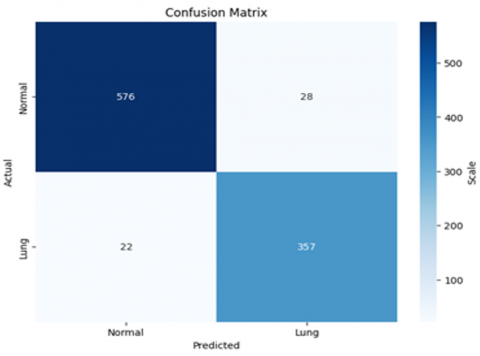
The designed model’s categorization efficiency was determined by estimating the confusion matrix. Figure 7 displays the confusion matrix of the presented technique. It is a tabular representation of the classifier's efficiency in categorizing lung cancer by comparing the classified outcomes with the real class. It also allows us to estimate the model's classification results such as accuracy, precision, recall, etc., through four cells namely: true positive (TP), true negative (TN), false positive (FP), and false negative (FN).
Figure 7. Confusion matrix
These cells evaluate the system's efficiency in correctly categorizing lung cancer and healthy instances from the images. TP indicates the case where it exactly classifies the lung cancer types, while TN defines the case where the system accurately detects and categorizes healthy images. In contrast, FP represents the case where the system incorrectly classifies the negative case as positive and FN denotes the case where it incorrectly categorizes the actual positive as negative.
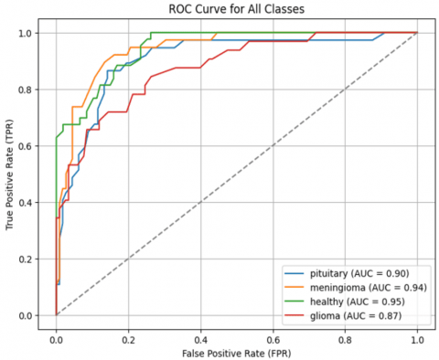
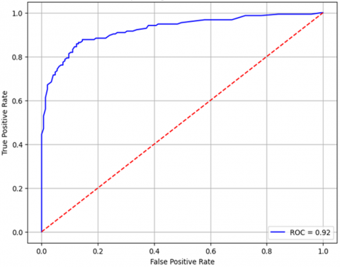
On the other hand, receiver operating characteristic (ROC) is the graphical illustration of the system’s classification results. It demonstrates how effectively the developed SWoCNN model categorizes lung cancer and healthy images across all possible thresholds. It is a plot of the TP rate against the FP rate, and it emphasizes the model's outcome by estimating the area under the curve (AUC). If AUC is close to 1, it indicates higher accuracy and vice versa.
Figure 8 displays the ROC curve of the presented model for 80/20 datasplit and 70/30 datasplit. It is observed that for 80/20 data split, the designed approach achieved AUC of 0.95, while for 70/30 data split it obtained AUC of 0.92. This higher AUC depicts that the designed framework precisely categorizes normal and lung cancer instances from the CT images.
(a)
(b)
Figure 8. ROC curve (a) 80/20 datasplit (b) 70/30 datasplit
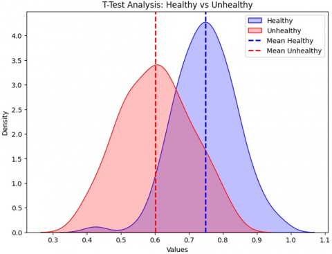
Furthermore, to validate the SWO optimization model, its convergence rate was compared with other optimization algorithms such as GA, PSO, GWO, and firefly optimization algorithm (FOA). The convergence rate quantifies how quickly the optimization algorithm converges to the optimal solution set per generation in the decision space (Figure 9).
Figure 9. Statistical significance analysis: (a) 80/20 data split, and (b) 70/30 data split
Figure 10 presents the comparative assessment of convergence curve of different optimization algorithms. Compared to other meta-heuristic optimization models, the proposed SWO approach achieved faster and highly stable convergence by reaching the best fitness score (lower training loss). This illustrates that utilizing SWO for CNN parameter fine-tuning results offer effective exploration and exploitation of search space and finds best value for each parameter.
Figure 10. Comparison of convergence curve of different optimization models
4.3 Comparative assessment
The performances achieved by the developed SWoCNN model were compared and evaluated with the conventional lung cancer classification algorithms such as Ant lion Optimized Multilayer Perception network (ALOMPN) [33], DenseNet [34], Attention-based CNN (AbCNN) [35], High ranking deep ensemble learning (HRDEL) [36] and Multilevel 3D Deep CNN (M3D-DCNN) [37].
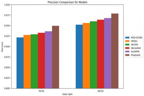
The metrics used in comparative analysis include accuracy, precision, FPR, f1-score, FNR, recall, computational time, and specificity, and these metrics are determined under two cases: 70/30 data split and 80/20 data split. Figures 11(a-d) present the comparative assessment of accuracy, precision, f1-score, and specificity. For 80/20 data split, the developed model and the existing techniques such as M3D-DCNN, HRDEL, AbCNN, DenseNet and ALOMPN obtained accuracy of 0.97872, 0.95238, 0.95634, 0.96436, and 0.96436, respectively, while for 70/30 dataset, these techniques earned accuracy of 0.94942, 0.92157, 0.92781, 0.93285, and 0.93629. This comparative analysis manifests that the developed methodology achieved improved accuracy than the conventional models, highlighting its proficiency in categorizing lung cancer from CT images. Similarly, the precision metric was compared with the existing models. The conventional classifiers and the presented SWoCNN achieved a precision of 0.95198, 0.95597, 0.96, 0.96406, 0.96815, and 0.97854, respectively for an 80/20 data split. On the other hand, they attained precision of 0.92153, 0.92773, 0.92930, 0.93282, 0.93624, and 0.94937, respectively for a 70/30 data split. The improvement of precision in the designed framework highlights its proficiency in recognizing the pattern of different lung cancer categories.
(a)
(b)
(c)
(d)
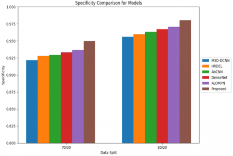
Figure 11. Performance comparison: (a) accuracy, (b) precision, (c) f1-score, and (d) specificity
Consequently, the designed strategy and the traditional models including M3D-DCNN, HRDEL, AbCNN, DenseNet and ALOMPN achieved f1-score of 0.98024, 0.95568, 0.95938, 0.96311, 0.96686, and 0.97065, respectively for 80/20 data split, while they earned f1-score of 0.94973, 0.92182, 0.92799, 0.92971, 0.93311, and 0.93682, respectively for 70/30 data split. The increased f1-score illustrates that the developed algorithm provides a balanced classification of healthy and lung cancer classes. The specificity of the model was also estimated and compared to the existing models to validate the efficiency of the designed SWoCNN model in recognizing the healthy image from tumor classes. The above-mentioned algorithm conventional models and the proposed framework achieved specificity of 0.95594, 0.95962, 0.96332, 0.96705, 0.97082, and 0.98035 for 80/20 data split, while they earned specificity of 0.92175, 0.92795, 0.92966, 0.93308, 0.93673, and 0.94971, respectively for 70/30 data split as shown in Table 2 and Table 3. The specificity comparison demonstrates that the developed model obtained greater specificity than the existing algorithms, which highlights its robustness in identifying and classifying normal images from the lung cancer-affected images.
Table 2. Comparative assessment of the developed model's performance with other techniques for an 80/20 ratio
|
Parameters |
M3D-DCNN |
HRDEL |
AbCNN |
DenseNet |
ALOMPN |
Proposed |
|
Accuracy |
0.95238 |
0.95634 |
0.96033 |
0.96436 |
0.96842 |
0.97872 |
|
Precision |
0.95198 |
0.95597 |
0.96 |
0.96406 |
0.96815 |
0.97854 |
|
Fl-Score |
0.95568 |
0.95938 |
0.96311 |
0.96686 |
0.97065 |
0.98024 |
|
Specificity |
0.95594 |
0.95962 |
0.96332 |
0.96705 |
0.97082 |
0.98035 |
|
Sensitivity |
0.95527 |
0.95900 |
0.96276 |
0.96655 |
0.97037 |
0.98005 |
|
FPR |
0.05772 |
0.05660 |
0.05172 |
0.04762 |
0.04412 |
0.04110 |
|
FNR |
0.03709 |
0.03614 |
0.03409 |
0.03226 |
0.03061 |
0.02913 |
|
Computational Time (Sec) |
20 |
19 |
15 |
15 |
13 |
7 |
Table 3. Comparative performance measures of the proposed model with other techniques
|
Parameters |
M3D-DCNN |
HRDEL |
AbCNN |
DenseNet |
ALOMPN |
Proposed |
|
Accuracy |
0.92157 |
0.92781 |
0.92934 |
0.93285 |
0.93629 |
0.94942 |
|
Precision |
0.92153 |
0.92773 |
0.92930 |
0.93282 |
0.93624 |
0.94937 |
|
F1-Score |
0.92182 |
0.92799 |
0.92971 |
0.93311 |
0.93682 |
0.94973 |
|
Specificity |
0.92175 |
0.92795 |
0.92966 |
0.93308 |
0.93673 |
0.94971 |
|
Sensitivity |
0.92172 |
0.92792 |
0.92963 |
0.93307 |
0.93669 |
0.94965 |
|
FPR |
0.05809 |
0.05749 |
0.05227 |
0.04846 |
0.04524 |
0.04312 |
|
FNR |
0.03824 |
0.03692 |
0.03690 |
0.03472 |
0.03160 |
0.03013 |
|
Computational Time (Sec) |
23 |
23 |
20 |
17 |
17 |
12 |
(a)
(b)
(c)
(d)
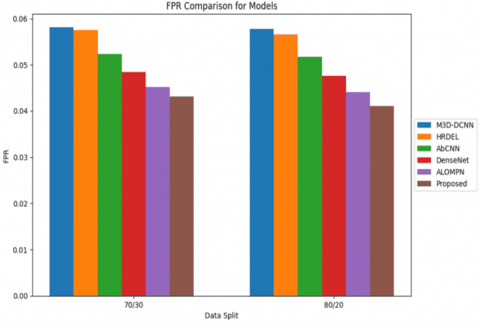
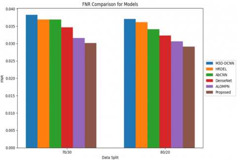
Figure 12. Performance comparison: (a) sensitivity, (b) FPR, (c) FNR, and (d) computational time
The comparative assessment of metrics such as sensitivity, FPR, FNR, and computational time are graphically presented in Figure 12. The sensitivity is a crucial parameter that determines the classifier's effectiveness in recognizing all correct (lung cancer instances) from the lung cancer cases that occurred. The presented methodology and the above-stated conventional models obtained a sensitivity of 0.94965, 0.92172, 0.92792, 0.92963, 0.3308, and 0.93673, respectively for 70/30 data split, while they achieved 0.98005, 0.95527, 0.95900, 0.96276, 0.96655, and 0.97037, respectively for 80/20 data split. The increased sensitivity in the designed model validates its effectiveness in identifying all lung cancer categories from both true and false positives. On the other hand, the FPR and FNR metrics are determined to estimate the error rate of the classifier. The designed strategy achieved lower FPR and FNR of 0.04312 and 0.03013 for the 70/30 data split, while it earned an FPR of 0.04110 and FNR of 0.02913 for the 80/20 data split. Subsequently, the above-mentioned conventional models achieved FPR of 0.5809, 0.05749, 0.05227, 0.04846 and 0.04524, and FNR of 0.03824, 0.03692, 0.03690, 0.03472, and 0.03160, respectively, for 70/30 data split. Also, they earned FPR of 0.05772, 0.05660, 0.05172, 0.04762, and 0.04412, and FNR of 0.03709, 0.03614, 0.03409, 0.03226, and 0.03061, respectively for 80/20 data split. The lower FPR and FNR in the developed algorithm highlight that it correctly classifies the healthy and lung cancer classes compared to existing models. Finally, the execution time is also determined to manifest the computational efficiency of the model. The presented algorithm consumed a minimum computational time of 7s and 12s for 80/20 and 70/30 data splits, while the existing models have taken longer computational times of the 20s, 19s, 15s, 15s, and 13s, respectively for 80/20 data split and 23s, 23s, 20s, 17s, and 17s, respectively for 70/30 data split. The reduced time consumption illustrates that the presented model quickly learns the feature representations and performs classification tasks. This also highlights that the parameter optimization by SWO minimizes the computational demands and training time. Tables 2 and 3 list the performance validation of the existing models with the presented approach for 80/20 and 70/30 data split.
4.4 Discussion
A hybrid classification strategy was developed to detect and classify the types of lung cancer from the CT images. The proposed model incorporates the optimization efficiency of SWO into the CNN to boost its adaptability and training speed through optimal parameter value selection. The presented work used the "Lung cancer CT scan database" from the Kaggle site as input and the images are preprocessed through steps like noise removal, image resizing, and background elimination. Also, the U-Net algorithm was developed to segment the ROI from the preprocessed images and the relevant features are captured using ANN. Consequently, a WPA-based feature selector was proposed to select the most informative and highly relevant attributes, assisting the classifier to focus on major features influencing the patterns of lung cancers. Finally, an optimized CNN was designed to perform the classification task. The CNN performs feature learning and estimates the lung cancer patterns by extracting spatial and local features. The SWO integrated into CNN refines its parameters continuously in an iterative manner, enabling the classifier to adapt to the evolving variations in input images and boosting the training speed through optimal parameter selection.
The robustness of the designed methodology was validated by determining the results in two cases: 80/20 and 70/30 data splits and the experimental results highlight that the designed methodology earned improved outcomes. Furthermore, a comparative assessment was performed with conventional classification models such as M3D-DCNN, HRDEL, AbCNN, DenseNet, and ALOMPN and it demonstrated that on average the performances such as accuracy, precision, recall, f1-score, and specificity are increased by 0.01172, 0.01176, 0.01132, 0.01132, and 0.01126 in the designed model. On the other hand, the metrics such as FPR, FNR, and computational time are reduced by 0.00257, 0.00123, and 5.5s in the presented methodology. The comparative analysis highlighted that the designed strategy performs better lung cancer classification than the currently available classifier model, making it a reliable solution to the real-time medical industry for early and precise lung cancer classification.
A lung cancer classifier SWoCNN was designed by combining the advantages of SWO into the CNN. The major objective of the research is to categorize the various types of lung cancer from the CT images using optimized CNN. The CT images are gathered from healthy and lung cancer-affected persons and preprocessed to make them suitable for further processes. Consequently, image segmentation and feature extraction are done using U-Net and ANN to capture ROI and relevant features from the preprocessed CT scans. A feature selector was designed using WPA to optimally select the most relevant and informative attributes from the extracted sequences. Finally, the proposed SWoCNN classifier was trained using the selected features to classify healthy and lung cancer categories such as adenocarcinoma, LCC, and SCC. The implementation outcomes of the designed strategy demonstrate that it achieved an accuracy of 0.94942 and 0.97872 for lung cancer classification on 70/30 and 80/20 data split. Furthermore, the developed approach earned a minimum execution time of 7s and 12s, demonstrating its computational efficiency. Finally, the comparative assessment with the existing techniques such as M3D-DCNN, HRDEL, AbCNN, DenseNet, and ALOMPN demonstrated that the designed framework achieved better outcomes than others.
Although the designed model achieved improved results, it has several limitations. Firstly, the presented strategy is limited to binary classification; it doesn’t classify the sub classes or different grades of lung cancer. Secondly, the developed framework is not validated across diverse databases, which limits its scalability across different clinical scenarios. Thirdly, the study has not focused on predicting the survival rate of cancer-affected individuals, which is crucial for preparing treatment plans. Hence future work focus on testing the scalability of the model and extending it to classify different lung cancer grades and predicting the survival rate of the patients.
[1] Jadhav, S.P., Singh, H., Hussain, S., Gilhotra, R., Mishra, A., Prasher, P., Krishnan, A., Gupta, G. (2021). Introduction to lung diseases. In Targeting Cellular Signalling Pathways in Lung Diseases, pp. 1-25.
[2] Huang, J., Deng, Y., Tin, M.S., Lok, V., Ngai, C.H. et al. (2022). Distribution, risk factors, and temporal trends for lung cancer incidence and mortality: A global analysis. Chest, 161(4): 1101-1111. https://doi.org/10.1016/j.chest.2021.12.655
[3] Zhou, R.X., Liao, H.J., Hu, J.J., Xiong, H., Cai, X.Y., Ye, D.W. (2024). Global burden of lung cancer attributable to household fine particulate matter pollution in 204 countries and territories, 1990 to 2019. Journal of Thoracic Oncology, 19(6): 883-897. https://doi.org/10.1016/j.jtho.2024.01.014
[4] Kumar, S., Kumar, H., Kumar, G., Singh, S.P., Bijalwan, A., Diwakar, M. (2024). A methodical exploration of imaging modalities from dataset to detection through machine learning paradigms in prominent lung disease diagnosis: A review. BMC Medical Imaging, 24(1): 30. https://doi.org/10.1186/s12880-024-01192-w
[5] Thanoon, M.A., Zulkifley, M.A., Mohd Zainuri, M.A.A., Abdani, S.R. (2023). A review of deep learning techniques for lung cancer screening and diagnosis based on CT images. Diagnostics, 13(16): 2617. https://doi.org/10.3390/diagnostics13162617
[6] Dafni Rose, J., Jaspin, K., Vijayakumar, K. (2020). Lung cancer diagnosis based on image fusion and prediction using CT and PET image. In Signal and Image Processing Techniques for the Development of Intelligent Healthcare Systems, pp. 67-86. https://doi.org/10.1007/978-981-15-6141-2_4
[7] Gu, C., Dai, C., Shi, X., Wu, Z., Chen, C. (2022). A cloud-based deep learning model in heterogeneous data integration system for lung cancer detection in medical industry 4.0. Journal of Industrial Information Integration, 30: 100386. https://doi.org/10.1016/j.jii.2022.100386
[8] Masud, M., Sikder, N., Nahid, A.A., Bairagi, A.K., AlZain, M.A. (2021). A machine learning approach to diagnosing lung and colon cancer using a deep learning-based classification framework. Sensors, 21(3): 748. https://doi.org/10.3390/s21030748
[9] Rana, M., Bhushan, M. (2023). Machine learning and deep learning approach for medical image analysis: Diagnosis to detection. Multimedia Tools and Applications, 82(17): 26731-26769. https://doi.org/10.1007/s11042-022-14305-w
[10] Kanan, M., Alharbi, H., Alotaibi, N., Almasuood, L., Aljoaid, S., Alharbi, T., Albraik, L., Alothman, W., Aljohani, H., Alzahrani, A., Alqahtani, S., Kalantan, R., Althomali, R., Alameen, M., Mufti, A. (2024). AI-driven models for diagnosing and predicting outcomes in lung cancer: A systematic review and meta-analysis. Cancers, 16(3): 674. https://doi.org/10.3390/cancers16030674
[11] Prabhu, S., Prasad, K., Robels-Kelly, A., Lu, X. (2022). AI-based carcinoma detection and classification using histopathological images: A systematic review. Computers in Biology and Medicine, 142: 105209. https://doi.org/10.1016/j.compbiomed.2022.105209
[12] Bhattacharjee, A., Murugan, R., Goel, T. (2022). A hybrid approach for lung cancer diagnosis using optimized random forest classification and K-means visualization algorithm. Health and Technology, 12(4): 787-800. https://doi.org/10.1007/s12553-022-00679-2
[13] Dritsas, E., Trigka, M. (2022). Lung cancer risk prediction with machine learning models. Big Data and Cognitive Computing, 6(4): 139. https://doi.org/10.3390/bdcc6040139
[14] Idrees, R., Abid, M., Raza, S., Kashif, M., Waqas, M., Ali, M., Rehman, L. (2022). Lung cancer detection using supervised machine learning techniques. https://www.researchgate.net/publication/364360173_Lung_Cancer_Detection_using_Supervised_Machine_Learning_Techniques.
[15] Cripsy, J.V., Divya, T. (2023). Lung cancer disease prediction and classification based on feature selection method using Bayesian network, logistic regression, J48, random forest, and Naïve Bayes algorithms. In 2023 3rd International Conference on Smart Data Intelligence (ICSMDI), Trichy, India, pp. 335-342. https://doi.org/10.1109/ICSMDI57622.2023.00066
[16] Rane, J., Mallick, S.K., Kaya, O., Rane, N.L. (2024). Scalable and adaptive deep learning algorithms for largescale machine learning systems. Future Research Opportunities for Artificial Intelligence in Industry, 4: 39-92.
[17] Rai, H.M., Yoo, J. (2023). A comprehensive analysis of recent advancements in cancer detection using machine learning and deep learning models for improved diagnostics. Journal of Cancer Research and Clinical Oncology, 149(15): 14365-14408. https://doi.org/10.1007/s00432-023-05216-w
[18] Surendar, P. (2021). Diagnosis of lung cancer using hybrid deep neural network with adaptive sine cosine crow search algorithm. Journal of Computational Science, 53: 101374. https://doi.org/10.1016/j.jocs.2021.101374
[19] Asuntha, A., Srinivasan, A. (2020). Deep learning for lung Cancer detection and classification. Multimedia Tools and Applications, 79(11): 7731-7762. https://doi.org/10.1007/s11042-019-08394-3
[20] Faruqui, N., Yousuf, M.A., Whaiduzzaman, M., Azad, A.K.M., Barros, A., Moni, M.A. (2021). LungNet: A hybrid deep-CNN model for lung cancer diagnosis using CT and wearable sensor-based medical IoT data. Computers in Biology and Medicine, 139: 104961. https://doi.org/10.1016/j.compbiomed.2021.104961
[21] Biradar, V.G., Pareek, P.K., Nagarathna, P. (2022). Lung cancer detection and classification using 2D convolutional neural network. In 2022 IEEE 2nd Mysore Sub Section International Conference (MysuruCon), Mysuru, India, pp. 1-5. https://doi.org/10.1109/MysuruCon55714.2022.9972595
[22] Bangare, S.L., Sharma, L., Varade, A.N., Lokhande, Y.M., Kuchangi, I.S., Chaudhari, N.J. (2022). Computer-aided lung cancer detection and classification of CT images using convolutional neural network. In Computer Vision and Internet of Things, pp. 247-262.
[23] Pandit, B.R., Alsadoon, A., Prasad, P.W.C., Al Aloussi, S., Rashid, T.A., Alsadoon, O.H., Jerew, O.D. (2023). Deep learning neural network for lung cancer classification: enhanced optimization function. Multimedia Tools and Applications, 82(5): 6605-6624. https://doi.org/10.1007/s11042-022-13566-9
[24] Mohandass, G., Krishnan, G.H., Selvaraj, D., Sridhathan, C. (2024). Lung cancer classification using optimized attention-based convolutional neural network with DenseNet-201 transfer learning model on CT image. Biomedical Signal Processing and Control, 95: 106330. https://doi.org/10.1016/j.bspc.2024.106330
[25] Yan, C., Razmjooy, N. (2023). Optimal lung cancer detection based on CNN optimized and improved Snake optimization algorithm. Biomedical Signal Processing and Control, 86: 105319. https://doi.org/10.1016/j.bspc.2023.105319
[26] Lin, C.H., Lin, C.J., Li, Y.C., Wang, S.H. (2021). Using generative adversarial networks and parameter optimization of convolutional neural networks for lung tumor classification. Applied Sciences, 11(2): 480. https://doi.org/10.3390/app11020480
[27] Lung cancer CT scan dataset. at https://www.kaggle.com/datasets/borhanitrash/lung-cancer-ct-scan-dataset, accessed on Dec. 10, 2024.
[28] Siddique, N., Paheding, S., Elkin, C.P., Devabhaktuni, V. (2021). U-net and its variants for medical image segmentation: A review of theory and applications. IEEE Access, 9: 82031-82057. https://doi.org/10.1109/ACCESS.2021.3086020
[29] Zhang, J., Zheng, B., Gao, A., Feng, X., Liang, D., Long, X. (2021). A 3D densely connected convolution neural network with connection-wise attention mechanism for Alzheimer's disease classification. Magnetic Resonance Imaging, 78: 119-126. https://doi.org/10.1016/j.mri.2021.02.001
[30] Abdelhamid, A.A., Towfek, S.K., Khodadadi, N., Alhussan, A.A., Khafaga, D.S., Eid, M.M., Ibrahim, A. (2023). Waterwheel plant algorithm: A novel metaheuristic optimization method. Processes, 11(5): 1502. https://doi.org/10.3390/pr11051502
[31] Li, Z., Liu, F., Yang, W., Peng, S., Zhou, J. (2021). A survey of convolutional neural networks: Analysis, applications, and prospects. IEEE Transactions on Neural Networks and Learning Systems, 33(12): 6999-7019. https://doi.org/10.1109/TNNLS.2021.3084827
[32] Abdel-Basset, M., Mohamed, R., Jameel, M., Abouhawwash, M. (2023). Spider wasp optimizer: A novel meta-heuristic optimization algorithm. Artificial Intelligence Review, 56(10): 11675-11738. https://doi.org/10.1007/s10462-023-10446-y
[33] Rojas, M.G., Olivera, A.C., Vidal, P.J. (2024). A genetic operators-based ant lion optimiser for training a medical multi-layer perceptron. Applied Soft Computing, 151: 111192. https://doi.org/10.1016/j.asoc.2023.111192
[34] Lanjewar, M.G., Panchbhai, K.G., Charanarur, P. (2023). Lung cancer detection from CT scans using modified DenseNet with feature selection methods and ML classifiers. Expert Systems with Applications, 224: 119961. https://doi.org/10.1016/j.eswa.2023.119961
[35] Mohandass, G., Krishnan, G.H., Selvaraj, D., Sridhathan, C. (2024). Lung cancer classification using optimized attention-based convolutional neural network with DenseNet-201 transfer learning model on CT image. Biomedical Signal Processing and Control, 95: 106330. https://doi.org/10.1016/j.bspc.2024.106330
[36] Pradhan, K.S., Chawla, P., Tiwari, R. (2023). HRDEL: High ranking deep ensemble learning-based lung cancer diagnosis model. Expert Systems with Applications, 213: 118956. https://doi.org/10.1016/j.eswa.2022.118956
[37] Tyagi, S., Talbar, S.N. (2023). LCSCNet: A multi-level approach for lung cancer stage classification using 3D dense convolutional neural networks with concurrent squeeze-and-excitation module. Biomedical Signal Processing and Control, 80: 104391. https://doi.org/10.1016/j.bspc.2022.104391