Dian Puspita Hapsari*![]() | Eka Mala Sari Rochman
| Eka Mala Sari Rochman![]() | Miswanto
| Miswanto![]() | Yuli Panca Asmara
| Yuli Panca Asmara![]() | Aeri Rachmad
| Aeri Rachmad![]() | Wahyudi Setiawan
| Wahyudi Setiawan![]()
© 2025 The authors. This article is published by IIETA and is licensed under the CC BY 4.0 license (http://creativecommons.org/licenses/by/4.0/).
OPEN ACCESS
In deep learning, particularly with convolutional neural networks (CNNs), overfitting is a common challenge, especially when training data is scarce. CNNs usually need large amounts of training data to avoid overfitting when working with new datasets. However, there is often not enough disease data available. To address this, using the right architecture is crucial for accurate disease prediction. In this study, we optimized our models using the adaptive moment estimation (ADAM) algorithm, which efficiently handles multiple parameters and requires less memory. The test scenario was structured with two primary objectives. The first objective was to evaluate the regularization and convergence of the CNN classifier model. A model is deemed convergent when it attains an acceptable level of error and regularization. The second objective was to assess the overall performance of the model utilizing metrics such as accuracy, precision, recall, and F1-score. We compared five CNN architectures and found that ShuffleNet achieved the highest accuracy at 98%, followed by EfficientNet at 96% and MobileNet at 93%. Although these architectures showed similar performance, the quality of input images significantly affects disease localization. Additionally, deep learning models are sensitive to noise, which can hinder performance. Future efforts will focus on enhancing prediction accuracy, class imbalance and model robustness.
osteoarthritis, X-ray image, deep learning, convolutional neural networks, ADAM, model performance metrics
Knee osteoarthritis (OA) is one of the most common joint disorders globally, affecting millions of people, particularly older adults. Its progression leads to pain, decreased mobility, and a lower quality of life, with knee OA being especially prevalent. Early detection of OA is vital for improving patient outcomes, and radiographic analysis is essential for diagnosis and staging. Manual diagnosis using X-ray imaging is not only time-consuming but also susceptible to subjectivity. Therefore, the development of automated diagnostic systems is imperative. These systems can significantly assist radiologists in accurately and efficiently identifying and grading the severity of OA [1].
Recent advances in deep learning, especially convolutional neural network (CNN), have shown remarkable potential for medical image analysis, enabling automated feature extraction and classification [2, 3]. CNN architectures like AlexNet, ResNet, and newer, lightweight models like EfficientNetV2 and MobileNetV2 have already proven effective in a variety of tasks, including medical image classification. When properly optimized, CNN models can achieve superior performance compared to conventional image processing techniques, offering significant improvements in both accuracy and processing speed [4, 5]. This capability makes CNNs particularly well-suited for applications in medical diagnostics [6]. Specifically, by developing a CNN-based system tailored for the diagnosis of knee OA, we could significantly enhance existing diagnostic workflows [7].
Such a system would not only provide rapid results but also ensure high reliability and reproducibility, fundamentally changing the way knee OA is diagnosed and managed in clinical settings. This paper presents a research inquiry centered on evaluating the performance of CNN classifiers across five distinct architectures—AlexNet, EfficientNetV2, MobileNetV2, ResNet, and ShuffleNet—for classifying knee OA severity in X-ray images. To enhance model performance, we will employ the Adaptive Moment Estimation (ADAM) optimization technique, which dynamically adjusts learning rates and has shown success in optimizing complex deep learning models [8]. This research seeks to identify the most effective CNN architecture for OA classification from X-ray images, considering both model accuracy and computational efficiency [9]. Our hypothesis is that the new architecture using Pointwise Group Convolution and Channel Shuffle design will perform better than the traditional CNN model architecture in predicting the X-ray image dataset. The findings could inform the development of robust, helping clinicians make more accurate diagnoses.
This study is dedicated to the task of classifying the severity of osteoarthritis through a detailed analysis of knee X-ray images. Osteoarthritis, a degenerative joint disease, can lead to significant pain and mobility issues, and accurately determining its severity is crucial for effective treatment planning. Image classification plays a vital role in this process, as it involves the sorting and categorization of images based on specific characteristics that define various degrees of osteoarthritis severity [10]. These characteristics can include factors such as joint space narrowing, bone spurs, and other radiographic indicators evident in the X-rays. To create a highly accurate classification model for the digital images, it is essential to utilize an effective algorithm capable of processing the intricate details present in the X-ray images [11].
In this research, we implemented both traditional image classification architectures, which have been widely used in past studies, and modern deep learning architectures, which offer advanced capabilities in feature extraction and pattern recognition. To enhance the performance of these models, we applied the Adam Optimizer, known for its efficiency and effectiveness in training neural networks [12, 13]. By leveraging both conventional and state-of-the-art approaches, this study aims to improve the accuracy and reliability of knee X-ray image classifications. Ultimately, this research not only seeks to provide clearer insights into the severity of osteoarthritis but also to contribute to better patient outcomes through more informed clinical decision-making.
2.1 CNN
A CNN is an essential architecture in deep learning, specifically engineered for the recognition and analysis of patterns in structured data, particularly images. CNNs are highly adept at automatically learning spatial hierarchies of features, which makes them exceptionally effective for image classification and object detection. The evolution of CNN architectures has been significant, leading to the development of groundbreaking variants that enhance both performance and efficiency. These advancements have driven major breakthroughs in deep learning, resulting in precise applications across critical fields like computer vision, healthcare, and autonomous systems. With each new variant, CNNs continue to push the limits of what artificial intelligence can achieve [14, 15]. The CNN-modeling has following two parts, feature learning and classification.
2.1.1 Feature learning
Feature learning empowers machines to automatically discover and harness the unique characteristics of input images, transforming raw data into insightful knowledge [16]. In CNN, the features are extracted through two components: convolution layer and pooling layer.
Convolution layer
The convolution layer serves as a powerful tool for feature extraction. By applying the convolution function followed by an activation function, it unlocks the potential of data. With multiple convolution layers, we harness deeper insights and elevate the art of feature extraction [17]. In the convolution operation, a fundamental technique used in signal processing and image analysis, we employ a linear function known as the kernel function to effectively extract features from the input data. This kernel function, which can also be referred to as the filter, acts as a sliding window, moving across the input data to identify important patterns and structures. By applying the kernel to various regions of the data, we generate a new representation that highlights specific features, such as edges or textures, which are crucial for further analysis and interpretation. This process is essential in computer vision, where it helps in tasks like object detection and image classification. Suppose we have an input image described by tensor I of dimension $m_1 * m_2 * m_c$, where,
$m_1=$ height of image
$m_2=$ width of image
$m_c=$ number of channels
We apply a filter which is also a tensor of dimension ($n_1 * n_2 * n_c$). The kernel is designed to have the same number of channels as the input image. As the filter traverses the image from left to right, it performs a multiplication operation between the corresponding sections of the image (I) and the kernel (K), summing the resulting products. The stride parameter specifies the increment by which the filter shifts as it scans the image. The resultant of I and K is another tensor of dimension $\left(m_1-n_1+1\right) *\left(m_2-n_2+1\right) * 1$.
$\begin{aligned} & \operatorname{dim} \text { of } I=m_1 * m_2 * m_c \\ & \operatorname{dim} \text { of } K=n_1 * n_2 * n_c \\ & \operatorname{dim} \text { of } F=\left(m_1-n_1+1\right) *\left(m_2-n_2+1\right) * 1\end{aligned}$
And,
$F[i, j]=(I * K)_{[i, j]}$
The ij-th entry of the feature map is given as below:
$f[i, j]=\sum_x^{m_1} \sum_y^{m_2} \sum_z^{m_c} K_{[x, y, z]} I_{[i+x-1, j+y-1, z]}$
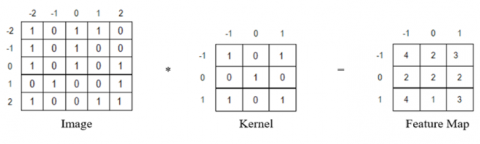
We have taken the following example of a 5×5×1 dimensional image being convoluted with a kernel of 3×3×1 and the stride s=1 has been used (Figure 1).
Figure 1. Feature extraction in convolution operation
The ij-th entry of feature map is given by following general formula in case of single channel:
$f[i, j]=(I * K)_{[i, j]}=\sum_x^{m_1} \sum_y^{m_2} K_{[x, y]} I_{[i-x, j-y]}$
The remaining entries can be derived utilizing the specified formula. This process is repeated by applying a variety of filters that extract distinct features from the image, such as blur and sharpness. It is important to note that multiple filters may be employed concurrently, which illustrates the concept of stride.
Padding
The procedure outlined previously has a significant limitation: the filters applied during processing tend to concentrate their effects more on the central areas of the image rather than on the corners. This uneven distribution of attention can lead to incomplete or distorted representations of the entire image, particularly affecting the areas that are not at the center. To address this issue, padding can be utilized. Padding is a technique that involves adding extra pixels around the edges of the input tensor before processing it with filters. Zero padding, in particular, is a widely used method in which a row and a column of zeros are added to each side—top, bottom, left, and right—of the input tensor. This approach not only helps maintain the dimensionality of the output but also ensures that the filters can adequately analyze and capture features located near the corners of the image, thereby improving overall image quality and feature detection.
Activation function
Typically, a bias term denoted as b is incorporated into the convolutional component prior to the application of the activation function.
$\begin{aligned} & c=F+b \\ & c=I * K+b \\ & \operatorname{Conv}(I, K)=\phi_a(c)=\phi_a(I * K+b)\end{aligned}$
where, $\phi_a$ is an activation function.
There are a variety of activation functions utilized in neural networks, including sigmoid, tangent, and hyperbolic tangent functions. Among these, the Rectified Linear Unit (ReLU) activation function is the most prevalent due to its efficiency in eliminating negative values:
$R(x)=\max (0, x)$
Pooling layer
In the pooling layer, the spatial dimensions of the features obtained from the convolution layer are intentionally reduced. This reduction process emphasizes the most prominent features of the image, allowing for a more efficient analysis. The pooling function is applied to the output produced by the convolution layer to facilitate this transformation.
Let us assume that:
$\begin{aligned} & \operatorname{Conv}(\boldsymbol{I}, \boldsymbol{K})=C \\ & P=\phi_p(C)\end{aligned}$
where, $\phi_p$ is a pooling function.
The dimension of pooled part is given as:
$\operatorname{dim} o f P=\left(\frac{m_1+2 p-n_1}{s}\right) *\left(\frac{m_2+2 p-n_2}{s}\right) * m_c$
where,
$\begin{aligned} & m_1 * m_2={ the \,dimension\, of \,input\, image, } \\ & n_1 * n_2={ the\, dimension\, of\, padding\, kernel, } \\ & s={ stride\, and\, p } ={ padding } .\end{aligned}$
There are several types of pooling methods utilized in deep learning, including sum pooling, average pooling, and max pooling. An illustration of max pooling is provided below. In this approach, max pooling is performed on 2×2 patches, selecting the maximum value from each patch.
2.1.2 Classification
To effectively extract features from the input data, multiple hidden layers are employed, specifically a combination of convolutional layers and pooling layers. These layers work together to identify and isolate important patterns and characteristics within the data. Upon the completion of the feature extraction process, the resulting multidimensional data is systematically transformed into a single one-dimensional vector through a process known as flattening. The optimized vector is utilized as the input for the fully connected layer, which is responsible for executing the final classification of the data based on the features that have been extracted [18, 19].
Fully connected layer
The fully connected layer plays a crucial role in processing the flattened vector, which is the output of the previous layer in a neural network. This layer transforms the input into another vector, allowing the model to learn complex relationships and representations within the data. In machine learning, it's common for different classes to be represented unevenly; some may occur more frequently than others, leading to potential bias in the model's predictions. To mitigate this imbalance, balanced weights are introduced in conjunction with the pooled data, ensuring that all classes are fairly represented. Furthermore, a bias term is added to stabilize the learning process, and this is followed by the application of an activation function, which introduces non-linearity and helps the model better fit the underlying patterns in the data.
The mathematical description is as below:
$\begin{aligned} & X=\sum_i w_i P_i+b \\ & z=g(X)\end{aligned}$
where, g is an activation function for the fully connected layer.
In this approach, each layer incorporates the weights associated with the pooled segments, enhancing the data representation. After the weights are applied, the activation function is activated, introducing non-linearity into the model. Several hidden layers are employed, allowing for complex feature extraction and transformation. In the final layer, a specific activation function is utilized to carry out the classification task, calculating the probabilities for each class and determining the most likely category for the input data [20].
2.2 Optimizer
The Adam algorithm represents a significant advancement in the field of optimization techniques. It was introduced by Sadu et al. [21]. This algorithm functions as a robust tool for stochastic optimization, recognized for its effectiveness in identifying optimal solutions even in the presence of randomness. One of the standout features of Adam is its requirement for only first-order gradients, making it remarkably efficient in terms of computational resources while utilizing minimal memory [21]. To grasp the concept of stochastic optimization more clearly, it's helpful to compare it to the well-known Stochastic Gradient Descent (SGD) method. SGD is highly effective for tasks that involve large datasets and a multitude of parameters. At each iteration, this method estimates the gradient by drawing a random subset of the data, known as a mini-batch. This approach allows SGD to converge toward optimal solutions more quickly compared to traditional Gradient Descent, which relies on evaluating the gradient using the entire dataset at every step. Consequently, SGD can handle large volumes of data efficiently, making it a popular choice in various machine-learning applications [22, 23].
The algorithm to optimize an objective function $f(\theta)$, with parameters $\theta$ (weights and biases).
Adam should incorporate the relevant hyperparameters: $\alpha$, $\beta 1$ (from Momentum), $\beta 2$ (from RMSProp).
Initialize:
$m=0$, this document presents the first moment vector, which is examined within the framework of momentum.
$v=0$, this represents the second moment vector, approached in a manner analogous to the RMSProp technique.
$t=0$
On iteration $t$:
Update $t, t=t+1$
Calculate the gradients or derivatives $(g)$ in relation to $t$. In this context, $g$ is equivalent to $d w$ and $d b$, respectively
$g_t=\operatorname{grad}\left(\theta_{t-1}\right)$
Update the first moment $m_t$
Update the second moment $v_t$
$\begin{aligned} & m_t=\beta_1 * m_{t-1}+\left(1-\beta_1\right) * g_t \\ & v_t=\beta_2 * v_{t-1}+\left(1-\beta_2\right) * g_t^2\end{aligned}$
Calculate the bias-corrected value $m_t$ (Implementing bias correction enhances the accuracy of estimates for moving averages).
Compute the bias-corrected $v_t$
$\begin{aligned} & \widehat{m}_t=\frac{m_t}{\left(1-\beta_1^2\right)} \\ & \hat{v}_t=\frac{v_t}{\left(1-\beta_2^2\right)}\end{aligned}$
Update the parameters $\theta$
$\theta_t=\theta_{t-1}-\alpha * \frac{\widehat{m}_t}{\sqrt{\hat{v}_t+\epsilon}}$
The loop will continue to execute until Adam successfully arrives at a solution.
Adam is widely recognized as one of the leading optimization algorithms in the field of machine learning, although it does have some limitations. Below are some of the key advantages and disadvantages associated with the Adam optimizer handling Sparse Gradients. Adam excels in managing sparse gradients, which often occur in noisy datasets. This makes it particularly effective for problems where data can be irregular or inconsistent. Robust Default Hyperparameters, one of the standout features of Adam is its default hyperparameter values, which tend to yield good results for a variety of machine learning tasks without the need for extensive tuning.
|
Algorithm 1 Stochastic Gradient Descent (SGD) |
|
1: Input: Initial point $x_0$, learning rate sequence $\left\{\eta_k\right\}$ 2: for $k=0,1,2, \ldots$ do 3: Sample $i_k$ uniformly at random 4: $x_{k+1}=x_k-\eta_k \nabla f_{i_k}\left(x_k\right)$ 5: end for |
Computational Efficiency, algorithm 1 is designed to be computationally efficient, making it suitable for training models quickly, even on complex tasks. For adaptive methods, we assume:
Adam: $\beta_1, \beta_2 \in[0,1)$ with $\beta_1<\sqrt{\beta_2}$
Memory efficiency, Adam utilizes memory effectively, requiring only a small footprint. This makes it an excellent option for environments with limited memory resources [24-26]. Performance on large datasets, the optimizer performs exceptionally well when applied to large datasets, enabling faster training times and the ability to work with more complex models. These characteristics make Adam a popular choice among practitioners looking for an effective optimization method in their machine learning projects.
3.1 Data collection
The Osteoarthritis Initiative (OAI) is a significant research project in the United States, offering a comprehensive dataset on osteoarthritis accessible via the NIMH Data Archive website at https://nda.nih.gov/oai. This dataset includes 8,260 records collected from 4,796 male and female participants aged 45 to 79 years, each meticulously categorized according to the severity of osteoarthritis as determined by clinical evaluations and imaging studies. The records are classified into five distinct target classes based on the degree of joint degeneration observed. Grade 0 (3,253 records): This classification signifies healthy joints without any evidence of osteoarthritis. These records serve as the baseline for comparative studies, highlighting the absence of disease progression in this group. Grade 1 (1,495 records): This category indicates the presence of very mild osteoarthritis symptoms, which might include minor structural changes or initial signs of cartilage degradation that are often unnoticed in daily activities.
Grade 2 (2,175 records): Representing moderate osteoarthritis, this group contains records where patients may begin to experience noticeable limitations in range of motion and discomfort during physical activities due to the deterioration of cartilage and the formation of bone spurs. Grade 3 (1,086 records): This classification points to more severe osteoarthritis, characterized by significant joint damage. Patients in this group often face marked pain and functional impairment, as the cartilage is considerably worn down, leading to more prominent bone-on-bone contact. Grade 4 (251 records): The most advanced stage, Grade 4, indicates severe osteoarthritis, with extensive joint destruction and significant pain. Patients may struggle with daily activities and may require surgical interventions, such as joint replacement, due to the debilitating nature of their condition.
This detailed categorization of records not only enhances our understanding of osteoarthritis progression but also provides invaluable data for researchers and healthcare professionals aiming to develop targeted treatments and interventions for individuals affected by this common degenerative joint disease. Target Class Descriptions our dataset: Grade 0 - Not Detected Osteoarthritis: This classification is characterized by the absence of any signs of osteoarthritis, as indicated by the green line. Grade 1 - Doubtful Osteoarthritis: This stage is identified by the presence of osteophyte formation and visible joint narrowing within the knee. Grade 2 - Mild Osteoarthritis Detected: This grade is characterized by the formation of osteophytes, represented in blue, alongside a potential narrowing of the joint space. Grade 3 - Moderate Osteoarthritis Detected: This classification is marked by the presence of numerous osteophytes (shown in blue) and joint space narrowing with accompanying sclerosis, indicated in purple. Grade 4 - Severe Osteoarthritis Detected: This stage signifies the presence of multiple enlarged osteophytes and is characterized by significant joint space narrowing and sclerosis.
Figure 2. Classification of knee OA severity with the Kellgren-Lawrence standard
Figure 2 showcases the five distinct target classes related to knee OA images. These classes represent varying levels of severity as defined by the Kellgren-Lawrence grading system. This standard evaluates the condition based on three key criteria: the presence and extent of osteophytes (bone spurs), the degree of narrowing in the joint space, and observable alterations in the structure of the bone. The table below offers a comprehensive description of each target class, providing insight into their specific characteristics and implications for diagnosis and treatment. Given the significant imbalance present in the data, it has been partitioned into training, testing, and validation sets, with careful consideration of the number of available samples for each category.
The dataset utilized for this analysis is imbalanced, meaning that some classes have significantly fewer samples than others. To address this issue, we implement an additional step to compute class weights or sample weights. Sample weights are essential as they assign a specific weight to each training sample, allowing the model to prioritize learning from underrepresented classes. In addition to sample weights, we also calculate class weights, which modify the loss function during training. This adjustment ensures that the model gives greater importance to the classes that are less frequently represented in the dataset, thus mitigating the effects of imbalance.
To effectively apply the calculated weights, we use a 2D array structure, which allows us to assign different weights for each timestep across every sample. The process begins with calculating the sample weights based on the distribution of classes in the training data. Following the computation of the weights, we proceed to define the model architecture, ensuring that it is capable of handling the specific requirements of the imbalanced dataset. Once the model is established, we adjust it by incorporating the previously calculated sample weights during each epoch of training. For our training regimen, we set the number of epochs to 20 and use a batch size of 32, facilitating a balanced approach to model training while accommodating the impact of class imbalance. This detailed methodology aims to enhance the model's performance on the minority classes, ultimately leading to improved overall accuracy.
3.2 Analysis
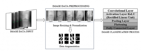
This section provides a comprehensive overview of the research process involved in classifying digital images of OA of the knee, utilizing the CNN algorithm. The various stages of this methodology, from data collection to classification, are detailed and visually represented in Figure 3, highlighting the systematic approach taken to achieve accurate classification of the images.
Figure 3. Image data preprocessing
Figure 4. The CNN classifier workflows
In Figure 4, the CNN classifier workflows define the architecture of a CNN by carefully selecting various types of layers, including convolutional layers, pooling layers, and fully connected layers. Convolutional layers are responsible for extracting features from the input images by applying filters, which help in identifying patterns and textures. Pooling layers, on the other hand, reduce the dimensionality of the feature maps and help in maintaining the most important information while decreasing computational complexity.
Finally, fully connected layers integrate features extracted by the previous layers and perform the final classification or regression task. To optimize the performance of the CNN, experiment with different architectural configurations. This could involve varying the number of layers, the size and number of filters in convolutional layers, the type of pooling (e.g., max pooling or average pooling), and the number of neurons in fully connected layers. It is essential to strike a balance between complexity and performance, ensuring that the model is neither too simple to underfit the data nor too complex to overfit. Regularization techniques and dropout can also be employed to enhance the model’s generalization capabilities.
This research is organized into several key stages, with a primary focus on:
3.2.1 Preprocessing
Preprocessing serves as a vital foundational step that transforms raw image data into a suitable format for input into a CNN. This stage is essential for ensuring that the data is ready for effective analysis and learning. It typically encompasses the following crucial operations:
1. Image Resizing: To achieve uniformity across the dataset, images are resized to a consistent dimension. This step is important because CNN architectures are designed to accept inputs of fixed sizes, and maintaining uniform dimensions allows for efficient processing and reduces complications during training.
2. Normalization: In this step, pixel values are normalized, commonly by scaling them to a range between 0 and 1. Normalization is beneficial as it accelerates the training process and enhances model performance. By ensuring that all input features are treated equally, normalization allows the model to learn more effectively and helps prevent biases that could arise from large variations in pixel intensity.
3. Data Augmentation: To enrich the training dataset and increase its diversity, various techniques such as rotation, flipping, and cropping are applied to the images. Data augmentation plays a critical role in improving the robustness of the model. By enabling the model to learn from a wider array of examples, this technique helps mitigate the risk of overfitting, allowing the model to generalize better when faced with new, unseen data.
Through these preprocessing steps, the dataset becomes more prepared for the complexities of training a CNN, ultimately supporting more accurate and reliable outcomes.
3.2.2 k-fold cross validation
k-fold cross-validation is a valuable technique for evaluating the performance of classifier models, including CNNs. It helps ensure that the classifier generalizes well to unseen data by providing a more reliable estimate of performance. In k-fold cross-validation, the dataset is divided into k non-overlapping subsets, or "folds." Each fold is used once as a validation set while the remaining k-1 folds are used for training. This process allows for multiple model evaluations, resulting in more accurate performance estimates on unseen data. Additionally, k-fold cross-validation can help reduce bias and variance. By averaging the results across all k folds, this method addresses the issues associated with relying on a single training/testing split. In the context of medical data prediction, bias is not expected; however, its presence could lead to decreased accuracy in predictions. This technique is particularly important in deep learning, where the risk of overfitting to a specific training dataset is high if proper validation is not conducted. k-fold cross-validation maximizes the use of available data, which is especially beneficial in scenarios where the dataset is limited, as every observation is used for both training and validation across multiple folds.
3.2.3 The image classification
The image classification process in CNNs consists of a series of meticulously designed layers, each playing a crucial role in extracting and interpreting information from images:
1. Convolutional Layer: Serving as the backbone of CNNs, the convolutional layer employs a set of learnable filters, commonly referred to as kernels. These filters slide across the input image, performing mathematical operations that reveal essential features such as edges, textures, and intricate shapes. As each filter processes the image, it generates a corresponding feature map, effectively highlighting specific patterns and characteristics that are vital for understanding the content of the image.
2. Activation Layer (ReLU): Following the convolution operation, the output undergoes a transformation through a nonlinear activation function, typically the ReLU. This step is critical as it introduces non-linearity into the model, enabling it to capture complex relationships within the data. By ensuring that negative values are set to zero while positive values remain unchanged, ReLU allows the network to learn more intricate patterns, enhancing its overall capability to differentiate between various features in the input image.
3. Pooling Layer: The pooling layer acts as a dimensionality reduction mechanism, streamlining the vast amount of information contained in the feature maps. By utilizing methods like max pooling, where the layer scans through the feature map and retains only the highest value from each segment, the pooling layer minimizes the computational burden. This not only conserves resources but also helps prevent overfitting, ensuring that the model generalizes well to unseen data by focusing on the most salient features.
4. Flattening: Once the pooling process is complete, the multidimensional feature maps are transformed into a one-dimensional vector in a step called flattening. This transformation is essential for transitioning to fully connected layers, as it converts the rich, high-dimensional data into a more manageable format that can be easily processed by subsequent neural network components.
5. Fully Connected Layer: In the fully connected layer, each neuron is intricately linked to every neuron in the preceding layer. This comprehensive connectivity allows the layer to aggregate and synthesize information from all extracted features, weighing them appropriately to formulate predictions about the class of the input image. The aggregation of this information is crucial for the model’s ability to render accurate classifications. The final output layer typically employs a SoftMax activation function for multi-class classification tasks. This function computes the probabilities of the input image belonging to each class, enabling the model to provide clear and interpretable predictions about the image's content.
The knee OA dataset comprises five distinct labels and is intended for multi-class classification within this study. A confusion matrix is generated through the classification process, which employs various architectural models. In a multi-class confusion matrix, the classification results are organized such that each element's predicted class (denoted by columns) is compared with its actual class (denoted by rows). Correctly classified elements are reflected on the diagonal, where the predicted class aligns with the true class, while non-diagonal elements represent the instances of misclassification. A greater count in the diagonal entries indicates superior performance of the classifier. Notably, the EfficientNetV2 CNN architecture demonstrated the highest number of correctly classified elements when compared to other conventional CNN architectures.
4.1 Convergency classification model
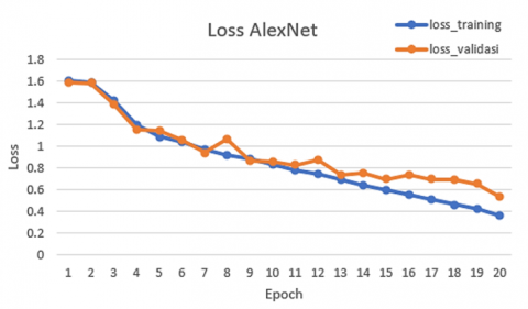
Overfitting is a significant issue encountered in model training, where excessive specialization of the training data adversely affects the model's capacity to generalize to new, unseen data. This phenomenon results in an escalation of generalization error, which can be accurately assessed through the model's performance on a validation data set. In this study, the utilization of the Adam optimizer is intended to facilitate the development of the most effective classifier model.
Figure 5 illustrates that both the training loss and validation loss demonstrate a consistent downward trend, subsequently stabilizing at a designated point. This observation indicates that the AlexNet architecture is a suitable fit for the data being analyzed.
Figure 5. Loss training and validation AlexNet
Figure 6. Loss training and validation ResNext50
In contrast to AlexNet, the training and validation loss metrics for ResNet50 (Figure 6) generally indicate that the model is experiencing overfitting and is unable to generalize effectively to new data. Specifically, the model demonstrates strong performance on the training dataset, while exhibiting weak performance on the validation set. Notably, there exists a point at which the validation loss decreases, only to subsequently increase once more.
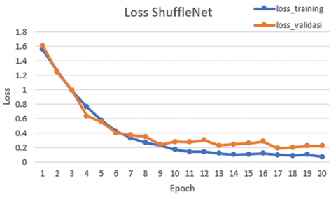
Figure 7 illustrates the training loss and validation loss associated with each convolutional neural network (CNN) architecture utilized in this study. The graph reveals that an effective model is characterized by both the training and validation losses exhibiting a decline until they reach a stable point, with a minimal disparity between their final values.
Figure 7. Loss training and validation MobileNet v2
Training loss and validation loss are critical metrics utilized to evaluate a model's performance and its capacity for generalization. Training loss represents the error associated with the data on which the model was trained. In contrast, validation loss assesses the error on previously unseen data, providing insights into the model's performance beyond the training dataset. By analyzing both metrics, one can gain a comprehensive understanding of the model's effectiveness.
Figures 7 and 8 illustrate that the graphs for MobileNet and ShuffleNet exhibit notable similarities, which suggest an optimal fit for both models. This indicates that neither model is experiencing overfitting nor underfitting.
Figure 8. Loss training and validation ShuffleNet v2
It is essential to acknowledge that the model loss consistently demonstrates lower values on the training dataset compared to the validation dataset. Consequently, some degree of separation between the learning curves of the training and validation losses is to be anticipated; this difference is commonly referred to as the "generalization gap."
Figure 9. Loss training and validation EfficientNet v2
In Figure 9, EfficientNet v2 exhibits a considerable degree of fitness, which suggests that it achieves an optimal fit—indicating that the model neither overfits nor underfits the data. Among the five CNN classifier architectures evaluated, EfficientNet demonstrates superior performance. A learning curve is deemed to reflect a successful match if: - The training loss continually decreases and subsequently stabilizes. - The validation loss similarly decreases, stabilizes, and maintains a minor gap relative to the training loss. Among the five architectures examined, EfficientNet demonstrates the most advantageous performance in comparison to the others.
4.2 Classification performance matric
CNN classifiers depend on the utilization of metrics to assess and evaluate model performance. These metrics serve as an objective means to determine the effectiveness with which a model learns patterns from the training dataset and applies them to previously unobserved data, such as validation and testing datasets. Furthermore, metrics are instrumental in facilitating the comparison of performance across various models or methodologies, thereby aiding in the selection of the model that best meets the specified requirements and objectives.
Table 1 indicates that the highest values across all metrics are observed in non-traditional architectures, specifically ShuffleNet and EfficientNet, both of which attained a score of 95% for each metric evaluated.
Table 1. Accuracy, precision, recall, and F1 score
|
Measure |
AlexNet |
ResNext50 |
MobileNet v2 |
ShuffleNet |
EfficientNet v2 |
|
Accuracy |
84.20% |
91.60% |
87.90% |
95.30% |
95.50% |
|
Precision |
84.50% |
91.60% |
88.40% |
95.50% |
95.50% |
|
Recall |
84.20% |
91.60% |
87.90% |
95.30% |
95.50% |
|
F1 score |
84.20% |
91.60% |
87.90% |
95.30% |
95.40% |
Figure 10. Models’ performance metrics
The findings of this study are comprehensively illustrated in Figure 10, where we analyze five key performance metrics: accuracy, precision, recall, and F1-score. These metrics are crucial for assessing the effectiveness of the models in classification tasks. In our evaluation, we examined five distinct CNN architectures, each designed with unique features and training strategies. Among these, ShuffleNet and EfficientNet emerged as the top performers, consistently attaining the highest scores across all metrics evaluated.
The high accuracy of these architectures indicates their ability to correctly classify a significant proportion of the data. Moreover, their impressive precision reflects a low rate of false positives, showcasing their reliability in making positive identifications. The strong recall scores suggest that both models are highly effective at identifying true positive cases, minimizing false negatives. Lastly, the balanced F1-scores display an overall robust performance, highlighting their suitability for tasks requiring both high precision and recall. Overall, the results suggest that ShuffleNet and EfficientNet are not only efficient in their computational designs but also excel in practical applications where performance metrics are critical for success.
From the results of the experiments that have been carried out and referring to the performance metrics, the performance of the ShuffleNet architecture can be described as follows. ShuffleNet is characterized by a sophisticated architecture that utilizes pointwise group convolutions and channel shuffle operations to enhance efficiency while maintaining accuracy. This advanced design results in fewer parameters and lower computational complexity compared to traditional neural network architectures. With a computational cost of 10 to 150 MFLOPs, ShuffleNet achieves approximately a 13-fold speedup without compromising accuracy. Furthermore, it exhibits improved performance metrics in classification tasks while necessitating significantly fewer resources. These attributes make ShuffleNet particularly suitable for deployment in environments with constrained resources.
The recall score is an important metric that indicates the number of correct predictions made by the model relative to the total number of data points positively diagnosed with the disease. As illustrated in Figure 11, the ShuffleNet CNN architecture demonstrates the highest recall score among the evaluated models. This indicates that it exhibits superior performance in prediction tasks. The significance of the precision score in relation to the recall score is contingent upon the specific application at hand. For instance, within the context of a medical diagnosis system, achieving high recall is often paramount. This approach prioritizes the identification of as many positive cases of diseases as possible, even if it results in some false positives, which may lead to unnecessary testing.
Figure 11. Recall score for ShuffleNet and EfficientNet
The results of this study are visually represented in Figure 10, which emphasizes the recall scores derived from the analysis of the knee OA dataset. This dataset is crucial for understanding the prevalence and characteristics of knee OA, as it encompasses a range of patient data and clinical outcomes. In examining the results, it becomes evident that both ShuffleNet and EfficientNet have emerged as the leading models, demonstrating exceptional performance with a recall score of 95%. This remarkable figure indicates that these models are highly proficient at identifying true positive cases, thereby effectively minimizing false negatives. The ability to accurately detect cases of knee OA is essential for timely diagnosis and intervention, underscoring the significance of these models in enhancing clinical decision-making and improving patient outcomes.
The implementation of CNNs in clinical workflows presents several challenges that must be addressed for successful deployment. CNNs require substantial volumes of high-quality, accurately annotated datasets for training. However, in clinical environments, the availability of such data can be quite limited. Additionally, acquiring image data poses its own difficulties, as varying patient conditions may lead to suboptimal image quality. This impact on data quality necessitates comprehensive preprocessing, which can be time-consuming and resource-intensive. Furthermore, data interoperability issues can emerge, given that different healthcare systems may utilize incompatible formats or standards. Another significant concern is algorithmic bias and the generalization of CNN models. The performance of these models can be adversely affected by biases present in the training datasets, potentially limiting their effectiveness across diverse patient populations and clinical scenarios. Therefore, ensuring that the model maintains the ability to generalize across various demographic groups is essential for its clinical applicability and utility.
In this paper, we employ deep learning-based classification techniques to evaluate knee OA as observed in X-ray images. We present new state-of-the-art results in the automatic classification of knee OA across all stages of severity. Moreover, we enhance the performance of our model through the implementation of gradient-based algorithm optimization. This approach facilitates fast, early, and reliable assessments of knee X-rays, presenting medical practitioners with an effective alternative that conserves time. The automatic classification substantially improves the overall efficacy of our system. Additionally, the application of gradient-based optimization enables the resulting classifier model to rapidly achieve convergence.
Among the various metrics utilized to assess model performance, ShuffleNet is particularly distinguished, achieving an accuracy rate of 98%. This is followed by EfficientNet at 96%, MobileNet at 93%, ResNet at 89%, and AlexNet at 85%. The primary performance metrics evaluated include accuracy, precision, recall, and F1 score. ShuffleNet and EfficientNet demonstrate commendable performance when compared to other architectural designs, showcasing a more efficient and effective approach. The high accuracy achieved by these models provides a promising solution to the challenges associated with image data prediction through CNNs. Such predictive accuracy can significantly assist healthcare professionals in patient diagnosis. While these architectures exhibit comparable performance levels, it is important to note that the quality of input images plays a crucial role in disease localization. Furthermore, deep learning models are inherently sensitive to noise, which can adversely affect their performance. Looking ahead, we intend to integrate multiple datasets from diverse settings to further enrich our analyses. Future endeavors will aim to enhance prediction accuracy, address class imbalance, and improve the overall robustness of the models.
We would like to thank Prof. Dr. Aeri Rachmad, S.T., M.T. Trunojoyo University Madura for the direction of this research activity. We would like to thank the Adhi Tama Surabaya Institute of Technology for providing support for this research activity.
[1] Katz, J.N., Arant, K.R., Loeser, R.F. (2021). Diagnosis and treatment of hip and knee osteoarthritis: A review. JAMA, 325(6): 568-578. https://doi.org/10.1001/jama.2020.22171
[2] Mohammed, A.S., Hasanaath, A.A., Latif, G., Bashar, A. (2023). Knee osteoarthritis detection and severity classification using residual neural networks on preprocessed X-ray images. Diagnostics, 13(8): 1380. https://doi.org/10.3390/diagnostics13081380
[3] Tariq, T., Suhail, Z., Nawaz, Z. (2023). Knee osteoarthritis detection and classification using X-rays. IEEE Access, 11: 48292-48303. https://doi.org/10.1109/ACCESS.2023.3276810
[4] Heidari, M., Mirniaharikandehei, S., Khuzani, A. Z., Danala, G., Qiu, Y., Zheng, B. (2020). Improving the performance of CNN to predict the likelihood of COVID-19 using chest X-ray images with preprocessing algorithms. International Journal of Medical Informatics, 144: 104284. https://doi.org/10.1016/j.ijmedinf.2020.104284
[5] Rachmad, A., Sonata, F., Hutagalung, J., Hapsari, D., Fuad, M., Sari Rochman, E.M. (2023). An automated system for osteoarthritis severity scoring using residual neural networks. Mathematical Modelling of Engineering Problems, 10(5): 1849-1856. https://doi.org/10.18280/mmep.100538
[6] Wang, Y., Wang, X., Gao, T., Du, L., Liu, W. (2021). An automatic knee osteoarthritis diagnosis method based on deep learning: Data from the osteoarthritis initiative. Journal of Healthcare Engineering, 2021(1): 5586529. https://doi.org/10.1155/2021/5586529
[7] Yeoh, P.S.Q., Lai, K.W., Goh, S.L., Hasikin, K., Hum, Y.C., Tee, Y.K., Dhanalakshmi, S. (2021). Emergence of deep learning in knee osteoarthritis diagnosis. Computational Intelligence and Neuroscience, 2021(1): 4931437. https://doi.org/10.1155/2021/4931437
[8] Soydaner, D. (2020). A comparison of optimization algorithms for deep learning. International Journal of Pattern Recognition and Artificial Intelligence, 34(13): 2052013. https://doi.org/10.1142/S0218001420520138
[9] Hannibal, S., Jentzen, A., Thang, D.M. (2024). Non-convergence to global minimizers in data driven supervised deep learning: Adam and stochastic gradient descent optimization provably fail to converge to global minimizers in the training of deep neural networks with ReLU activation. arXiv preprint arXiv:2410.10533. https://doi.org/10.48550/arXiv.2410.10533
[10] Rachmad, A., Husni, Hutagalung, J., Hapsari, D., Hernawati, S., Syarief, M., Rochman, E.M.S., Rachmad, A., Hutagalung, J., Hapsari, D., Hernawati, S., Syarief, M., Rochman, E.M.S., Asmara, Y.P. (2024). Deep learning optimization of the EfficienNet architecture for classification of tuberculosis bacteria. Mathematical Modelling of Engineering Problems, 11(10): 2664-2670. https://doi.org/10.18280/mmep.111008
[11] Cabrejos-Yalán, V.M., Rodriguez, C. (2024). Convolutional neural network model for skin cancer diagnosis in a dermatological center. Mathematical Modelling of Engineering Problems, 11(11): 2997-3005. https://doi.org/10.18280/mmep.111112
[12] Thakur, S., Kumar, A. (2021). X-ray and CT-scan-based automated detection and classification of COVID-19 using convolutional neural networks (CNN). Biomedical Signal Processing and Control, 69: 102920. https://doi.org/10.1016/j.bspc.2021.102920
[13] Mahum, R., Rehman, S.U., Meraj, T., Rauf, H.T., Irtaza, A., El-Sherbeeny, A.M., El-Meligy, M.A. (2021). A novel hybrid approach based on deep CNN features to detect knee osteoarthritis. Sensors, 21(18): 6189. https://doi.org/10.3390/s21186189
[14] Khan, A.A., Laghari, A.A., Awan, S.A. (2021). Machine learning in computer vision: A review. EAI Endorsed Transactions on Scalable Information Systems, 8(32): e4. https://doi.org/10.4108/eai.21-4-2021.169418
[15] Heenaye-Mamode Khan, M., Boodoo-Jahangeer, N., Dullull, W., Nathire, S., Gao, X., Sinha, G.R., Nagwanshi, K.K. (2021). Multi-class classification of breast cancer abnormalities using deep convolutional neural network (CNN). PloS One, 16(8): e0256500. https://doi.org/10.1371/journal.pone.0256500
[16] Sikkandar, M.Y., Begum, S.S., Alkathiry, A.A., Alotaibi, M.S.N., Manzar, M.D. (2022). Automatic detection and classification of human knee osteoarthritis using convolutional neural networks. Computers, Materials & Continua, 70(3): 4279-4291. https://doi.org/10.32604/cmc.2022.020571
[17] Alzubaidi, L., Zhang, J., Humaidi, A.J., Al-Dujaili, A., et al. (2021). Review of deep learning: Concepts, CNN architectures, challenges, applications, future directions. Journal of Big Data, 8: 53. https://doi.org/10.1186/s40537-021-00444-8
[18] Yaqub, M., Feng, J., Zia, M.S., Arshid, K., Jia, K., Rehman, Z.U., Mehmood, A. (2020). State-of-the-art CNN optimizer for brain tumor segmentation in magnetic resonance images. Brain Sciences, 10(7): 427. https://doi.org/10.3390/brainsci10070427
[19] Kenneweg, P., Kenneweg, T., Hammer, B. (2024). Improving line search methods for large scale neural network training. In 2024 International Conference on Artificial Intelligence, Computer, Data Sciences and Applications (ACDSA), Victoria, Seychelles, pp. 1-6. https://doi.org/10.1109/ACDSA59508.2024.10467724
[20] Reyad, M., Sarhan, A.M., Arafa, M. (2023). A modified Adam algorithm for deep neural network optimization. Neural Computing and Applications, 35(23): 17095-17112. https://doi.org/10.1007/s00521-023-08568-z
[21] Sadu, S., Dubey, S.R., Sreeja, S.R. (2023). Moment centralization-based gradient descent optimizers for convolutional neural networks. In Computer Vision and Machine Intelligence, pp. 51-63. https://doi.org/10.1007/978-981-19-7867-8_5
[22] Junayed, M.S., Jeny, A.A., Islam, M.B., Ahmed, I., Shah, A.S. (2022). An efficient end-to-end deep neural network for interstitial lung disease recognition and classification. Turkish Journal of Electrical Engineering and Computer Sciences, 30(4): 1235-1250. https://doi.org/10.55730/1300-0632.3846
[23] Dubey, S.R., Singh, S.K., Chaudhuri, B.B. (2023). Adanorm: Adaptive gradient norm correction based optimizer for CNNs. In 2023 IEEE/CVF Winter Conference on Applications of Computer Vision (WACV), Waikoloa, HI, USA, pp. 5273-5282. https://doi.org/10.1109/WACV56688.2023.00525
[24] Bhatt, D., Patel, C., Talsania, H., Patel, J., et al. (2021). CNN variants for computer vision: History, architecture, application, challenges and future scope. Electronics, 10(20): 2470. https://doi.org/10.3390/electronics10202470
[25] Chakrabarti, K., Chopra, N. (2022). A control theoretic framework for adaptive gradient optimizers in machine learning. arXiv preprint arXiv:2206.02034. https://doi.org/10.48550/arXiv.2206.02034
[26] Wang, Y., Xiao, Z., Cao, G. (2022). A convolutional neural network method based on Adam optimizer with power-exponential learning rate for bearing fault diagnosis. Journal of Vibroengineering, 24(4): 666-678. https://doi.org/10.21595/jve.2022.22271