Nidhal Q. Saadoon![]() | Noora T. Abduirazzaq
| Noora T. Abduirazzaq![]() | Adel S. Hussain
| Adel S. Hussain![]() | Noora A. Mohammed
| Noora A. Mohammed![]() | Emad A. Az-Zo’bi
| Emad A. Az-Zo’bi![]() | Mohammad A. Tashtoush*
| Mohammad A. Tashtoush*![]()
© 2025 The authors. This article is published by IIETA and is licensed under the CC BY 4.0 license (http://creativecommons.org/licenses/by/4.0/).
OPEN ACCESS
This analysis aims to adapt the Heun’s numerical method integrated with a dual-Wiener process framework to solve fuzzy stochastic differential equations (FSDEs) by processing challenges faced by randomness and uncertainty. FSDEs incorporate stochastic processes with fuzzy parameters, such as triangular and trapezoidal fuzzy numbers, to model uncertainties arising from incomplete or imprecise data. The modified Heun’s method is a predictor-corrector scheme designed to enhance accuracy and computational stability, outperforming traditional methods like Euler-Maruyama. The main contributions include the combining of fuzzy arithmetic into stochastic models and the use of dual-Wiener processes to account for complex uncertainties. The study demonstrates theoretical convergence under fuzzy and stochastic conditions and validates its findings through numerical simulations. Results confirm the method’s strong and weak convergence, as well as its robustness in tackling FSDEs across applications in finance, engineering, and environmental modeling. Comparative analysis highlights significant error reduction, particularly in cases with larger sample sizes, underscoring the method’s efficacy. Our study bridges openings in numerical solutions for FSDEs by presenting an applicable and efficient approach for solving problems in systems with random and fuzzy parameters. Future work may focus on extending the methodology to higher-dimensional systems and integrating machine learning techniques to enhance performance further.
stochastic differential equations, Heun’s method with dual-wiener processes, fuzzy stochastic ordinary differential equations, trigonometric fuzzy numbers, numerical analysis, Brownian motion
In 1905, Einstein first introduced the concept of stochastic differential equations (SDEs), providing a mathematical description of Brownian motion by demonstrating the connection between the random behavior of small particles and the diffusion equation on a larger scale. Since then, these equations have become an indispensable tool in various fields such as physics, chemistry, biology and microelectronics, as well as in economics and finance. Traditionally, solutions of these equations have relied heavily on the Ito integration technique to achieve accuracy when dealing with stochastic phenomena. However, the exact methods face some challenges in solving non-trivial problems, which led to the resort to approximation methods as an alternative to overcome these difficulties, as discussed in study [1].
In many practical applications, data on parameters may be incomplete or distorted by measurement errors or mathematical approximations. These uncertainties lead to ambiguities in the differential equations used, which require more sophisticated methods for estimating the solutions. These uncertainties can be expressed using probabilistic or fuzzy for the simulation of complex natural phenomena [2-4].
Heun’s method, or Heun’s consistency method, is a numerical procedure for solving ordinary differential equations (ODEs) and is ideal for the order initial value problem. Compared to the simple Euler method, it is superior because of basic prediction and correct step strategies, where an interval with basic gradient is used and another interval is used to adjust constant gradients of that respective interval. Here, the constructive solution and a method that fits well are Heun’s method because of the lack of constructive solutions to fuzzy stochastic ordinary differential equations (FSODEs). In order to manage the existing uncertainty due to fuzzy parameters, the Heun’s method is integrated into the dual Wiener process within the course of the study. This makes it possible as an efficient numerical solution can be achieved, which could be utilized in several practical area of random occurrences and vagueness. Instead of that, this approach enhances the effectiveness of the solutions as well as the applicability of the numerical, as well as ansatz, methods in complex modeling situations [5-14].
In the past years, the combining of fuzziness with stochastic problems modeled by differential equations has earned attention in several fields of science, engineering, and finance. The fuzzy differential equations (FDEs) process the uncertainty that is found in real-world problems and can't be sufficiently represented by classical probabilistic models. Such models merge the flexibility of fuzzy theory and the randomness in the stochastic models.
The solutions key of FSDEs pass essentially through numerical methods that are used to derive approximate solutions. Among these methods, we focus our attention on the Heun's method, one of the second order Runge-Kutta schemes, which shows effectiveness in tackling generalized FSDEs. With low cost and high accuracy, this method is considered as an improvement of the Euler method. As well, the Heun's method assists in approximating the evolution of fuzzy quantities over time.
A critical component of stochastic models is the dual Wiener process, which expands the classical Brownian motion. In the study of complex systems, the dual Wiener process is an appropriate in modeling systems when multiple uncertainties need to be hold. In this analysis, we aim to examine the applicability of the Heun's method to FDEs obtained by dual Wiener processes.
The study of SFDEs has appeared in a wide range of research. In what follows, we mention the most recent studies regarding our contribution.
Jafari and Malinowski [15] focused on developing symmetric FSDEs driven by fractional Brownian motion to generalize models that incorporate both stochasticity and fuzziness in hybrid systems. They explored the existence of unique solutions under certain conditions and used a semi-martingale approximation method to show convergence of approximate solutions to the exact ones. The study also included an example on population dynamics, opening avenues for applications in fields like biology, finance, and mechanics.
The weak convergence of numerical schemes for SDEs with super-linear coefficients, which can cause moment blowup has been proved by Zhao et al. [16]. A systematic approach to analyze the weak error and convergence orders of explicit schemes, comparing truncation and balanced schemes through numerical experiments, has also been presented. The study aimed to improve the understanding of these methods, especially in cases where traditional approaches may struggle due to the challenges posed by super-linear coefficients. Iqbal et al. [17] have investigated fuzzy random differential equations, and also proved a random fixed-point theorem in fuzzy metric spaces. For more expansions and improvements, see the bibliography included therein.
The literature highlights significant advancements in the FSDEs as they also reveal the inadequacy of existing numerical solutions to handle stochastic and other complexities in actual applications. In response to these considerations, this research’s methodological approach combines Heun’s method with a dual Wiener process model. This enhances it applicability in fields like financial and environmental modeling will improve numerical stability and reliability and parameters are represented as fuzzy numbers. Our method provides clear solutions to the challenges presented by fuzzy SODEs; it avoids some of the shortcomings of previous work by focusing on these considerations.
2.1 Limitations in the fuzzy SODEs
Certain limitations can be pointed out at the article devoted to the numerical solution of FSODEs based on the Heun’s method. It is also important to note that this work is mostly developed for triangular and trapezoidal fuzzy numbers, meaning that other kinds of uncertainty may be treated with more difficulty by the proposed method, such as fuzzy intervals or fuzzy sets of higher order. Some textbooks define the stability of the numerical schemes only in terms of the growth or monotonicity with respect to the step size, without regards for the stability of the numbers in the chaotic or noisy environments; the accuracy of the numerical method relies on the precise definition of the initial conditions. This is compounded by the fact that it also lacks a rigorous validation of the method through examples to support the concept advanced by the authors of the study. While Heun’s method is superior due to this reason, there may be issues with computation involving the implementation of the integration method especially in high dimension or usage cases for real time processing. Furthermore, the defined Wiener processes may not possess independence which is wholly appropriate for all practical applications. And because there have been no prior comparison studies with other numerical methods, it is challenging to assess the pros and cons of Heun’s method. Thus, the purpose of this article is to present the findings along with an understanding of these study limitations so that anyone delivering, receiving, or interpreting these results will fully understand what exactly these results mean and for what kinds of purposes the results are useful. In turn, more research in the future will be useful to refine this method and expand the sphere where it can be applied.
In this paper, a sound approach for the approximate solution of stochastic differential equation problems in the fuzzy environment through Heun’s method for two Wiener process within the context of Ito’s Fuzzy Stochastic Integral model will be established with a provision of an exact solution. Fuzzy arithmetic for triangular fuzzy numbers is also performed, and the approximate solutions are shown to converge to the exact fuzzy solution through checking the conditions of the existence and uniqueness theorem of the problem stated.
3.1 Fuzzy sets and numbers
The fuzzy set ˇA contains pairs of elements and their associated membership functions. The membership function μ˜A is defined as follows:
μ˜A:X→[0,1] (1)
where, X is the universal set. A fuzzy number is defined as a convex natural set and is given as follows: The fuzzy number z in parametric form is a pair of values [k_,ˉk] of functions k_(α),ˉk(α), where α∈[0,1], which meets the following conditions [1]:
1. k_(α) it is a left-continuous, non-decreasing function bounded in the interval [0, 1], and right continuous at 0.
2. ˉk(α) it is a left-continuous, non-increasing function bounded in the interval (0,1], and right continuous at 0.
3. k_(α)≤ˉk(α),0≤α≤1.
A fuzzy number ˇA=[a,b,c] is said to be triangular when its membership function is given by:
μˇA(x)={0 if x≤ax−ab−a if a<x≤bc−xc−b if b<x<c1 if x≥c (2)
Consider the two fuzzy numbers ˜L=[L_(α),ˉL(α)] and ˜D=[D_(α),ˉD(α)] and a scalar d then:
1. ˜L=˜D if and only if L_(α)=D_(α) and ˉL(α)=ˉD(α).
2. ˜L+˜D=[L_(α)+D_(α),ˉL(α)+ˉD(α)].
3. ˜L−˜D=[L_(α)−D_(α),ˉL(α)−ˉD(α)].
4. d˜L={[dL_(α),dˉL(α)], if d≥0[dD_(α),dˉD(α)], if d<0
3.2 SDEs
Let's review a classical SDE [1]:
dxt=adt+bdw1+kdw2 (3)
where, Eq. (3) is expressed in differential form:
x(t2)−x(t1)=∫t2t1a(t,x)ds+∫t2t1b(t,x)dw1(s)+∫t2t1k(t,x)dw2(s) (4)
The last term on the right-hand side of Eq. (2) is known as the Ito integral. We will now take 0=t0<t1<t2<⋯<tn=T, be a grid of points on an interval [0, T], the Ito integrals are determined for each component separately, depending on the different components on the right-hand side of Eq. (4) is being:
∫t2t1b(t,x)dw(s)=∫tt0bi,j(s,xs)Δwi (5)
where, Δwi=wti−wti−1, transition in Brownian motion over a time interval.
Let us consider Eq. (5), which is first solved analytically using Ito's formula. According to this formula, if Xt represents the Ito process, then:
dξ(t)=adt+bdw(t) (6)
and let f(x, t) the function is continuous in (x,t)∈×[∞,0), along with its partial derivatives fx,fxx,ft. Then the process f(ξ(t),t). It is characterized by a random differential defined as follows:
df(ξ(t),t)=[ft(ξ(t),t)+fx(ξ(t),t)a(t,x)+12fxx(ξ(t),t)b2(t,x)]dt+fx(ξ(t),t)b(t,x)dw(t) (7)
3.3 Computational techniques for SDEs
To calculate the numerical solution of a SDEs, we define a grid of points, 0=t0<t1<t2<⋯<tn=T, and approximate x values w0<w1<w2<⋯<wn, it is determined at specific values of t. Consider the initial value problem of a SDE [1]:
{dXt=a(t,xt)dt+b(t,xt)dw1+k(t,xt)dw2X(0)=X0 (8)
where, a(t,xt),b(t,xt) and k(t,xt) are all continuous functions which are defined on interval [t0,T]. Where dw1,dw2 are wiener process with components w1t,w2t,…,wmt. Then Eq. (8) is solved numerically as follows.
3.4 Adaptation of Heun’s method for fuzzy parameters and dual-Wiener processes
The uncertainties associated with real-word applications of Heun’s method are handled by modifications to the method for fuzzy parameters and dual-Wiener processes. Heun’s method is a powerful predictor-corrector technique for solving numerical ODEs; the approach developed in this paper makes use of fuzzy numbers to describe uncertain parameters. This shift moves the original deterministic model to stochastic fuzzy environment and initial conditions and parameters are presented as triangular or trapezoidal fuzzy numbers [16-20].
Another improvement to the method is the addition of a combined dual-Wiener process approach that models stochastic system action using two separates but interacting Wiener processes. The predictor step of Heun’s method is modified to find solutions according to the fuzzy parameters and the corrector step amortize the solution by considering the stochasticity out of the dual-Wiener processes.
This combined adaptation enhances numerical precision and guarantees that the solutions captured consider uncertainty as well as stochastic nature making it advantageous in specific applications such as financial models, engineering failure analysis or environmental impact assessments.
Let us consider using a discrete-time approximation to estimate the Ito process in solving SDEs. Let us apply a discrete-time approximation to Eq. (8) to estimate the Ito process in solving SDEs.
x(x1)=x(x0)+∫x1x0a(s,xs)ds+∫tt0b(s,xs1)dws1+∫tt0k(s,xs2)dws2 (9)
Also let
I1=∫t=x1t0=x0a(s,xs)ds=∫t=x1t0=x0f(x)dx (10)
where, trapezoidal rule, x0=t0,x1=t,h=x0−x1=t0−t, and
f(x)=Pn(x)+fn+1(δ)(n+1)!∏ni=0(x−xi) (11)
Provided that
Pn(x)=∑ni=0i≠kf(xi)∗Li(x) (12)
where, the Lagrange equation is Li(x)=X−XiXk−Xi. And, also if n=1. Then:
P1(x)=∑1i=0i≠kf(xi)∗X−XiXk−Xi=X−X1X0−X1∗f(x0)+X−X0X1−X0∗f(x1) (13)
Hence:
f(x)=x−x1x0−x1∗f(x0)+x−x0x1−x0∗f(x1)+f(n+1)(ε)(n+1)!∏ni=0(x−xi) (14)
By substituting Eq. (14) into Eq. (10), we obtain:
I1=∫t=x1t0=x0(x−X1X0−X1∗f(x0)+x−X0X1−X0∗f(x1))dx+∫t=x1t0=x0f(n+1)(ε)(n+1)!∏ni=0(x−xi)dx (15)
Simplifying Eq. (14), we will get:
I1=∫t=x1t0=x0f(x)dx=∫t=x1t0=x0{(x−x1)22(x0−x1)∗f(x0)+(x−x0)22(x1−x0)∗f(x1)}dx=x1−x02[f(x0)+f(x1)]=h2[f(x0)+f(x1)] (16)
and
I2=∫tt0b(xs1)dws1=∫t=x1t0=x0b(s,xs1)dws1=∫t=x1t0=x0b(x)dws1=x1−x02[b(x0)+b(x1)] (17)
Additionally,
I3=∫tt0k(xs2)dws2=∫t=x1t0=x0k(s,xs1)dws2=∫t=x1t0=x0k(x)dws2=X1−X02[k(x0)+k(x1)] (18)
The Heun’s approx. is defined as cont. Time stochastic process. y={y(T);t0≤t<T} satisfying the iterative scheme: X0=x0:
xn+1=xn+h2[f(xn)+f(xn+aΔn+bΔwn)]Δn+h2[b(xn)+b(xn+aΔn+bΔwn)b(xn)+b(xn+aΔn+bΔwn)]Δwn1
+h2[k(xn)+k(xn+aΔn+bΔwn)]Δwn2 (19)
where,
Δti+1=ti+1−ti,ΔWi+1=W(ti+1)−W(ti)∼√ti+1−tiN(0,1)
where, N(0, 1) represents a standard normally distributed random variable with mean zero and variance one. The function randn (1, N), N random variables will be generated according to the standard normal distribution. To obtain a random variable with a given variance Δti+1, random variables with standard normal distribution are generated by a custom MATLAB function. randn (1, N). These variables are then multiplied by the result to obtain random increments in ΔWi+1.
3.5 Computational solutions for FSDEs
Suppose there are fuzzy parameters in a SDE; then Eq. (3) can be rewritten as:
d[X_(α),ˉX(α)]=[a_(α),ˉa(α)]dt+[b_(α),ˉb(α)]dw1+[k_(α),ˉk(α)]dw2 (20)
Eq. (10) is now solved using analytical and numerical methods respectively. By applying limit method, FSDE Eq. (10) can be reformulated explicitly and modified as follows [20]:
d[lim (21)
where,
\begin{gathered}X(\alpha)=\underline{X}(\alpha)+\frac{\bar{X}(\alpha)-\underline{X}(\alpha)}{s}, \\ a(\alpha)=\underline{a}(\alpha)+\frac{\bar{a}(\alpha)-\underline{a}(\alpha)}{s} \text { and } b(\alpha)=\underline{b}(\alpha)+\frac{\bar{b}(\alpha)-\underline{b}(\alpha)}{s}\end{gathered}
First, for the precise case, we use explicit representations of X(\alpha), a(\alpha) and b(\alpha), use Ito's integral to solve the problem. This version is more concise and clearly conveys the use of crisp representations and the Ito integral for solving the problem. If we apply the fuzzy concept we discussed earlier to the Heun’s method, Eq. (9) can be reformulated as follows.
\tilde{x}\left(x_1\right)=\tilde{x}\left(x_0\right)+\int_{x_0}^{x_1} a\left(s, \tilde{x}_s\right) d s+\int_{t_0}^t b\left(s, \tilde{x}_{s_1}\right) d w_{s_1}+\int_{t_0}^t k\left(s, \tilde{x}_{s_2}\right) d w_{s_2} (22)
The Heun’s approximation is defined as a continuous-time stochastic process, y=\left\{y(T) ; t_0 \leq t<T\right\}, that satisfies an iterative scheme. When applied to SDEs, the Heun's method is adapted to handle fuzzy parameters by incorporating triangular and trapezoidal fuzzy numbers. This approach enables the approximation of solutions to fuzzy SDEs, ensuring that the process accommodates the inherent uncertainty in the system. The resulting fuzzy Heun's method is essential for obtaining accurate solutions in systems where both randomness and fuzziness are presented:
X_0(\alpha)=w_0(\alpha)
w_{i+1}(\alpha)=w_i(\alpha)+\frac{h}{2}\left[f\left(w_i\right)+f\left(w_i+a\left(t_i, w_i, \alpha\right) \Delta t_{i+1}\right)+b\left(t_i, w_i, \alpha\right) \Delta w_i\right] \Delta t_{i+1}
\begin{aligned} & +\frac{h}{2}\left[b\left(w_i\right)+b\left(w_i+a\left(t_i, w_i, \alpha\right) \Delta t_{i+1}\right)+b\left(t_i, w_i, \alpha\right) \Delta w_n\right] \Delta w_{i_1} \\ & +\frac{h}{2}\left[k\left(w_i\right)+k\left(w_i+a\left(t_i, w_i, \alpha\right) \Delta t_{i+1}\right)+b\left(t_i, w_i, \alpha\right) \Delta w_i\right] \Delta w_{i_2}\end{aligned} (23)
where,
\begin{gathered}X_0(\alpha)=\underline{X_0}(\alpha)+\frac{\overline{X_0}(\alpha)-\underline{X_0}(\alpha)}{S}, \\ w_0(\alpha)=\underline{w_0}(\alpha)+\frac{\overline{w_0}(\alpha)-\underline{w_0}(\alpha)}{S}, \\ w_{i+1}(\alpha)=\underline{w_{i+1}}(\alpha)+\frac{\overline{w_{i+1}}(\alpha)-\underline{w_{i+1}}(\alpha)}{S}, \\ \mathrm{a}\left(t_i, w_i, \alpha\right)=\underline{\mathrm{a}}\left(t_i, w_i, \alpha\right)+\frac{\overline{\mathrm{a}}\left(t_i, w_i, \alpha\right)-\underline{\mathrm{a}}\left(t_i, w_i, \alpha\right)}{S}, \\ \underline{\mathrm{~b}}\left(t_i, w_i, \alpha\right)+\frac{\overline{\mathrm{b}}\left(t_i, w_i, \alpha\right)-\underline{\mathrm{b}}\left(t_i, w_i, \alpha\right)}{S} \\ \underline{\mathrm{k}}\left(t_i, w_i, \alpha\right)+\frac{\overline{\mathrm{k}}\left(t_i, w_i, \alpha\right)-\underline{\mathrm{k}}\left(t_i, w_i, \alpha\right)}{S} .\end{gathered}
Applying \lim _{s \rightarrow \infty} and \lim _{s \rightarrow 1} when we solve an equation, we get a left and a right term. We can also extract a number of different solutions by using different values of the membership function when \alpha \in[0,1]. Sometimes these solutions can be weak, leading to an overlap or intersection between the left and right terms due to the random nature of the system. This overlap can be clearly seen in the problems in the following examples.
3.6 Numerical stability analysis for Heun’s methods in fuzzy SODEs
We will discuss the two most common measures of stability: mean square and asymptotic [18-20]. Assuming that X_0 \neq 0 with probability 1, solutions of FSDE is:
d \tilde{X}_t=a\left(t, \tilde{x}_t\right) d t+b\left(t, \tilde{x}_t\right) d w_1+k\left(t, \tilde{x}_t\right) d w_2 (24)
Meeting the requirements of:
\lim _{t \rightarrow \infty} E X^2(t)=0 \leftrightarrow R\{\lambda\}+\frac{1}{2}|\mu|^2<0 (25)
\lim _{t \rightarrow \infty}|X(t)|=0 \leftrightarrow R\left\{\lambda-\frac{1}{2} \mu^2\right\}<0 (26)
The left side of Eq. (25) defines the concept of mean-square stability, while the right side of Eq. (25) describes this property in detail using the FSDE function. Similarly, Eq. (26) defines and describes asymptotic stability.
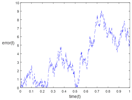
Two examples of SODEs which were originally formulated as crisp problems are discussed in this section in order to illustrate the concepts already introduced. All the parameters, which are to be determined in their CRT form, are later fuzzified using triangular and trapezoidal fuzzy numbers. Initially, the problem is analyzed for both crisp parameter values analytically and numerically and then for fuzzy parameter values. It is argued here that the selected examples satisfy the conditions in the existence and uniqueness of solutions to the fuzzy SODEs in studies [21-24]. Figure 1 shows Brownian paths at the unit interval [0,1] with sample sizes 100 and 1000 at the top and bottom respectively.
Figure 1. Discretized Brownian path
Example 1
Consider problem of solving the fuzzy SODE [1].
d \tilde{x}(t)=\tilde{x}\left(w_t\right) d t+\tilde{x}\left(w_t\right) d w_1(t)+k d w_2(t) (27)
with initial condition given as a triangular fuzzy number \tilde{X}_0(\alpha)=\widetilde{w}_0(\alpha). And k is positive constants. The exact solution of the crisp problem is given for comparison purpose as follows:
x(t)=\frac{x_0}{12} e^{\left(\frac{t}{2}+w_t\right)} (28)
Now, the Heun’s scheme for Eq. (25) is as follows:
\begin{gathered}X_0=w_0 \\ w_{i+1}=w_i+\frac{h}{2} \tilde{x} w_i \Delta t_{i+1}+\frac{h}{2} \tilde{x} \Delta w_{i_1}+\frac{k h}{2} \Delta w_{i_2}\end{gathered} (29)
Table 1. Explicit and fuzzy parameter values used in the study
|
Parameters |
Crisp |
Time (t) |
Fuzzy Value |
|
k |
0.2 |
0 |
[1,2,3] |
|
0.1 |
[1.1,2.1,3.1] |
||
|
0.2 |
[1.2,2.2,3.2] |
||
|
0.3 |
[1.3,2.3,3.3] |
||
|
0.4 |
[1.4,2.4,3.4] |
||
|
1.0 |
[1.5,2.5,3.5] |
Table 2. Error introduced by Huynh's method and comparison with Euler-Marauyam
|
r |
N |
Mean Squared Error (MSE) |
|
|
Heun’s Scheme |
Euler-Maruyama Scheme [25] |
||
|
1 |
50 |
0.1074 |
0.45512 |
|
100 |
0.0716 |
0.39665 |
|
|
1000 |
0.0186* |
0.20838 |
|
|
2 |
50 |
1.2074 |
1.6168 |
|
100 |
1.0716 |
1.5149 |
|
|
1000 |
1.1186 |
1.4093 |
|
Figure 2. Numerical solutions of FSDEs: comparison across Brownian motion sample sizes
Figure 2 shows the numerical behavior of the model, demonstrating its effectiveness in capturing the trends observed in the dataset.
Figure 3. Absolute error analysis of the fuzzy Heun’s method compared to the exact solution for n=1000, r=1
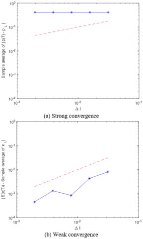
Figure 4. Fuzzy Heun’s strong and weak convergences
The values of the parameters used in Eq. (21) are specified in Table 1.
Absolute errors in the final time intervals for various sample sizes, where \Delta t=\delta t and r=1, are presented in Table 2 and Figure 3. In these results, the discretization steps of the Brownian motion align with the time steps used in the Heun scheme, compared to the Euler-Maruyama scheme. It is observed that increasing the sample size N leads to a reduction in absolute errors across different time steps. This indicates that larger sample sizes improve the accuracy of the numerical solution when \Delta t=\delta t.
From the Table 2, we observe that as the value of n increases from the smallest to the largest, the error value at the final point decreases.
Figure 4 illustrates how the strong and weak error varies with \Delta t on a log-log scale. For comparison, a dashed red reference line with a slope of one is provided. Power law of least squares analysis gives suitable results, q_1=0.5194, with a residual of 0.0355.
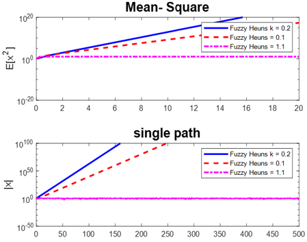
Figure 5 shows the sample mean E\left(\tilde{x}^2\right) against t. In this Figure, the curves for k=0.8 and k=0.2 increase with t, while the curve for k=1 decays toward zero.
Figure 5. Mean-square and asymptotic stability analysis of FSDEs
Example 2
The fuzzy SDE of Langevin equation is [24]
d \tilde{x}(t)=-\mu \tilde{x}(t) d t+\sigma d w_1(t)+k d w_2(t) (30)
with initial condition given as a triangular fuzzy number \tilde{X}_0(\alpha)=\widetilde{w}_0(\alpha). And \mu, \sigma and k are positive constants. The exact solution of the crisp problem is given for comparison purpose as follows:
x(t)=x_0 e^{\sigma w_1(t)+k w_2(t)+\left(\mu-\frac{\sigma^2+k^2}{2}\right) t} (31)
Now, the Heun’s scheme for Eq. (30) is as follows:
\begin{gathered}X_0=w_0 \\ w_{i+1}=w_i-\frac{\mu h}{2} \tilde{x} w_i \Delta t_{i+1}+\frac{\sigma h}{2} \Delta w_{i_1}+\frac{k h}{2} \Delta w_{i_2}\end{gathered} (32)
Figure 6 illustrates the numerical solutions of the fuzzy Langevin equation for different Brownian motion sample sizes, demonstrating the impact of sample size on the accuracy of the method. The values of the parameters used in Eq. (30) are specified in the following Table 3.
Figure 6. Numerical solutions of the fuzzy Langevin equation: analysis across Brownian motion sample sizes
Table 3. Explicit and fuzzy parameter values used in the study
|
Parameters |
Crisp |
TFN |
|
μ |
1.5 |
[1.4,1.5,1.6] |
|
σ |
0.25 |
[0.85,0.25,0.75] |
|
k |
0.1 |
[0.7,0.1,0.5] |
Table 4. Error introduced by Huynh's method and comparison with Euler-Marauyam
|
r |
N |
MSE |
|
|
Heun’s Scheme |
Euler-Maruyama Scheme [25] |
||
|
1 |
50 |
0.1074 |
0.45512 |
|
100 |
0.0716 |
0.39665 |
|
|
1000 |
0.0186* |
0.20838 |
|
|
2 |
50 |
1.2074 |
1.6168 |
|
100 |
1.0716 |
1.5149 |
|
|
1000 |
1.1186 |
1.4093 |
|
Absolute error in the final time period for various sample sizes, as shown in \Delta t=\delta t ; r=1 is presented in Table 4 and Figure 7. In these results, the discretization step for Brownian motion matches the time step used in the Heun’s scheme comparative with the Euler-Maruyama scheme. As observed, increasing the number of samples N leads to a reduction in absolute error across various time steps, demonstrating that a larger sample size improves the accuracy of the numerical solution when \Delta t=\delta_t.
From the Table 4, we observe that as the value of n increases from the smallest to the largest, the error value at the final point decreases, see Figure 7.
Figure 7. Absolute error evaluation of the fuzzy Heun’s method against the exact solution for n=1000, r=1
Figure 8. Analysis of strong and weak convergence of the fuzzy Heun’s method applied to the fuzzy Langevin equation
Figure 9. Mean-square stability and long-term asymptotic properties of FSDEs
Figure 8 shows how the strong error changes with Δt on a log-log scale. A red dashed reference line with a slope of one is included for comparison purposes, which is obtained using the law of least squares, q_2=0.2936, with residual 0.6243.
Figure 9 plots the sample average of E\left(\tilde{x}^2\right) against t. In this figure, the curves for k=0.2 and k=0.1 increase with t, while the curve for k=1.1 decays toward zero.
4.1 Discussion of results and anomalies
This section provides an in-depth analysis of the numerical results presented in Tables 2 and 4 and Figures 3 and 7. The analysis focuses on understanding the performance of the Fuzzy Heun’s method integrated with dual Wiener processes in solving FSODEs, highlighting the convergence behavior and the observed anomalies.
Table 2 depicts the following findings; the MSE reduces as the sample size N is increased. Furthermore, the graph also reveals, when comparing the MSE’s for the two simulations, that the MSE for N=1000 is noticeably higher than the MSE for N=50, which corroborates our previous observations, that is, larger sample sizes yield more accurate numerical solutions. This is in line with random theoretical assumptions where the variability of the approximate in stochastic simulations is normally reduced by enhancing the number of samples leading to smaller variations and improved stability. Therefore, it possible to conclude that the time step (\Delta t) is also an important factor that may influence the method’s accuracy. Whilst a bigger step size is easier to incorporate the differential equation into the iterative process, smaller step size would enable the achievement of better estimate for the solution hence decreasing the error. On the other hand, it would be expected that larger time steps generate higher errors because of the discrete nature of the approximation applied in Heun’s method. The choice of sample size and time step affects the sample’s computational cost and accuracy and has to be optimized for best performance.
One unexpected anomaly arises when comparing the results in Table 4, where the MSE for N=1000 in example 2 (the fuzzy Langevin equation) is not consistently smaller than for N=100. This counterintuitive result may arise from several factors:
FSODEs often involve non-linarites that can lead to higher errors at larger sample sizes. As the dimensionality of the system increases, especially with non-linear drift and diffusion terms, the method might struggle to maintain accuracy. Non-linear systems are particularly challenging for numerical methods as they amplify errors, especially when the system exhibits sensitive dependence on initial conditions.
Another reason for this effect may be random randomization that is inevitable for stochastic processes, for example, Wiener’s ones. For the large groups, the random error is more pronounced, and in some cases, this will cause more error. This is particularly true in those situations where the system under analysis is unnaturally sensitive to the initial conditions in other words where it exhibits a chaotic behavior in this respect even seemingly marginal changes to the common sample size or initial conditions may lead to disproportionately large changes in the results.
Some issues remain to be solved even if Heun’s method gives good stability on average; growing numerical instabilities in higher-dimensional space and higher-order fuzzy parameters may cause anomalies. Such instabilities can arise in the form random swings in the error at large sample sizes.
This section presents a detailed analysis of the convergence properties of the adapted fuzzy Heun’s method for solving stochastic differential equations. Both theoretical and experimental approaches are discussed to validate the method’s robustness.
4.2 Theoretical convergence analysis
The convergence of the numerical method is assessed based on the strong and weak convergence criteria for SDEs.
E\left[\left|Y_T-Y_{\text {exact }}(T)\right|^2\right]^{\frac{1}{2}} \leq C \Delta t^p (33)
where, Y_T is the numerical solution, Y_{\text {exact }}(T) is the exact solution, and \Delta t is the time step.
\left|E\left[Q\left(Y_T\right)\right]-E\left[Q\left(Y_{\text {exact }}(T)\right)\right]\right| \leq C \Delta t^p (34)
where, Q(x) is a smooth test function.
4.3 Experimental convergence tests
To verify convergence experimentally, we evaluate the method’s performance on test problems under varying discretization step sizes (\Delta t) and sample sizes (N).
M S E=\frac{1}{N} \sum_{i=1}^N\left(Y_T{ }^{(i)}-Y_{\text {exact }}{ }^{(i)}\right)^2 (35)
4.4 Results and discussion
4.5 Implications
The results validate the adapted Fuzzy Heun’s method as a robust tool for solving stochastic differential equations with fuzzy parameters, achieving acceptable convergence in both strong and weak senses.
In this study, a new numerical technique is developed for approximation of FSODEs with an integration of Heun’s method and dual Wiener processes. The major contributions include: Using triangular and trapezoidal fuzzy numbers to inject fuzziness, solving SODEs that cannot be solved to any productivity level using other approach. The method enhances both accuracy of solutions as well as the computational results and the potential has been established by convergence analysis and empirical evidence and it has been shown to be useful when solving more realistic problems such as fuzzy Langevin equations. This work fills voids that exist in earlier literature by presenting a feasible approach to model uncertainty in complicated stochastic structures, and has implications for practice in areas such as finance, engineering, and physics.
For possible future works, the method should be applied to higher-dimensional systems. Several nonlinearities including rational, periodic, and logarithmic nonlinearities should be included. In addition, such works may be considered to tackle complex nonlinear systems and integrating fuzzy logic with machine learning techniques, potentially artificial neural networks, to enhance solution accuracy.
The authors are very grateful to the Duhok of Polytechnic University for providing access which allows for more accurate data collection and improved the quality of this work.
[1] Arnold, L. (1974). Stochastic Differential Equations: Theory and Applications. John Wiley and Sons, Inc.
[2] Moore, R.E. (1966). Interval Analysis. Englewood Cliffs: Prentice-Hall, pp. 8-13.
[3] Malinowski, M.T. (2013). Some properties of strong solutions to stochastic fuzzy differential equations. Information Sciences, 252: 62-80. https://doi.org/10.1016/j.ins.2013.02.053
[4] Song, Y., Sohl-Dickstein, J., Kingma, D.P., Kumar, A., Ermon, S., Poole, B. (2020). Score-based generative modeling through stochastic differential equations. arXiv preprint, arXiv:2011.13456. https://doi.org/10.48550/arXiv.2011.13456
[5] Craigmile, P., Herbei, R., Liu, G., Schneider, G. (2023). Statistical inference for stochastic differential equations. Wiley Interdisciplinary Reviews: Computational Statistics, 15(2): e1585. https://doi.org/10.1002/wics.1585
[6] Moore, R.E., Kearfott, R.B., Cloud, M.J. (2009). Introduction to interval analysis. Society for Industrial and Applied Mathematics.
[7] Chakraverty, S., Tapaswini, S., Behera, D. (2016). Fuzzy Differential Equations and Applications for Engineers and Scientists. CRC Press.
[8] Shirawia, N.A.W.A.L., Kherd, A., Bamsaoud, S.A.L.I.M., Tashtoush, M., Jassar, A., Az-Zo’bi, E. (2024). Dejdumrong collocation approach and operational matrix for a class of second-order delay IVPs: Error analysis and applications. WSEAS Transactions on Mathematics, 23: 467-479. https://doi.org/10.37394/23206.2024.23.49
[9] Narváez, D.M.D., Mesa, F., Correa-Vélez, G. (2020). Numerical comparison by different methods (second order Runge Kutta methods, Heun method, fixed point method and Ralston method) to differential equations with initial condition. Scientia et Technica, 25(2): 299-305. https://doi.org/10.22517/23447214.24446
[10] Denis, B. (2020). An overview of numerical and analytical methods for solving ordinary differential equations. arXiv preprint, arXiv:2012.07558. https://doi.org/10.48550/arXiv.2012.07558
[11] Chupradit, S., Widjaja, G., Mahendra, S.J., Ali, M.H., Tashtoush, M.A., Surendar, A., Kadhim, M.M., Oudah, A.Y., Fardeeva, I., Firman, F. (2023). Modeling and optimizing the charge of electric vehicles with genetic algorithm in the presence of renewable energy sources. Journal of Operation and Automation in Power Engineering, 11(1): 33-38. https://doi.org/10.22098/joape.2023.9970.1707
[12] Zhang, Y., Huang, H., Li, J., Yang, M., Wu, S. (2019). Heun-thought Aided ZD4N g S method solving ordinary differential equation (ODE) including nonlinear ODE system. In Advances in Computational Science and Computing, Huangshan, China, pp. 460-471. https://doi.org/10.1007/978-3-030-02116-0_54
[13] Ibrahim, I., Taha, W., Dawi, M., Jameel, A., Tashtoush, M., Az-Zo’bi, E. (2024). Various closed-form solitonic wave solutions of conformable higher-dimensional fokas model in fluids and plasma physics. Iraqi Journal for Computer Science and Mathematics, 5(3): 401-417. https://doi.org/10.52866/ijcsm.2024.05.03.027
[14] Az-Zo’bi, E. A., Afef, K., Ur Rahman, R., Akinyemi, L., Bekir, A., Ahmad, H., Mahariq, I. (2024). Novel topological, non-topological, and more solitons of the generalized cubic p-system describing isothermal flux. Optical and Quantum Electronics, 56(1): 84. https://doi.org/10.1007/s11082-023-05642-7
[15] Jafari, H., Malinowski, M.T. (2023). Symmetric fuzzy stochastic differential equations driven by fractional Brownian motion. Symmetry, 15(7): 1436. https://doi.org/10.3390/sym15071436
[16] Zhao, Y., Wang, X., Zhang, Z. (2024). On one-step numerical schemes of weak convergence for SDEs with super-linear coefficients. arXiv preprint arXiv:2406.14065. https://doi.org/10.48550/arXiv.2406.14065
[17] Iqbal, M., Batool, A., Hussain, A., Alsulami, H. (2024). Fuzzy fixed-point theorems in S-metric spaces: Applications to navigation and control systems. Axioms, 13(9): 650. https://doi.org/10.3390/axioms13090650
[18] Zureigat, H., Tashtoush, M.A., Jassar, A.F.A., Az-Zo’bi, E.A., Alomari, M.W. (2023). A solution of the complex fuzzy heat equation in terms of complex Dirichlet conditions using a modified crank–Nicolson method. Advances in Mathematical Physics, 2023(1): 6505227. https://doi.org/10.1155/2023/6505227
[19] Malik Gul, U., Paul, A., Chee, K.W.A. (2022). Mathematical modeling of real-time systems using Heun and piecewise methods. Mathematical Problems in Engineering, 2022(1): 4651084. https://doi.org/10.1155/2022/4651084
[20] Qiu, Y., Chen, H. (2023). Exponential stability for neutral stochastic differential delay equations with Markovian switching and nonlinear impulsive effects. International Journal of Control, Automation and Systems, 21(2): 367-375. https://doi.org/10.1007/s12555-021-0283-x
[21] Sabri, R., Ahmed, B. (2023). Another type of fuzzy inner product space. Iraqi Journal of Science, 64(4): 1853-1861. https://doi.org/10.24996/ijs.2023.64.4.25
[22] Kandel, A. (1986). Fuzzy Mathematical Techniques with Applications. Addison-Wesley Longman Publishing Co., Inc.
[23] Djaouti, A., Liaqat, M. (2024). Qualitative analysis for the solutions of fractional stochastic differential equations. Axioms, 13(7): 438. https://doi.org/10.3390/axioms13070438
[24] Chandra, T., Yasin, M., Lailiyah, F. (2024). Numerical solution to the differential equation system of Lotka-Volterra by using Heun method. AIP Conference Proceedings, 3049(1): 020010. https://doi.org/10.1063/5.0194394
[25] Zhen, Y. (2024). Approximations of the Euler–Maruyama method of stochastic differential equations with regime switching. Mathematics, 12(12): 1819. https://doi.org/10.3390/math12121819
[26] Chupradit, S., Tashtoush, M., Ali, M., AL-Muttar, M., Sutarto, D., Chaudhary, P., Mahmudiono, T., Dwijendra, N., Alkhayyat, A. (2022). A multi-objective mathematical model for the population-based transportation network planning. Industrial Engineering & Management Systems, 21(2): 322-331. https://doi.org/10.7232/iems.2022.21.2.322