Vjayan Chandrasekaran | Manimaran Rajendran* | Racshitha Nagarajan
© 2025 The authors. This article is published by IIETA and is licensed under the CC BY 4.0 license (http://creativecommons.org/licenses/by/4.0/).
OPEN ACCESS
In this study, we introduce a novel semi-analytical technique, the Conformable Shehu Homotopy Analysis Transform Method (CSHAM), designed to solve the two-dimensional Black-Scholes equation. The method integrates the homotopy analysis method with the conformable fractional Shehu transform (CST), a Laplace-type integral transform that extends the capabilities of traditional Laplace and Sumudu transforms. The Shehu transform offers easy-to-use properties and simpler visualization compared to Sumudu and other natural transforms. We establish the convergence analysis of the method and demonstrate its applications to fractional diffusion equations, confirming its efficiency and high accuracy. The results obtained using CSHAM are in complete accordance with those obtained using existing techniques, affirming its effectiveness.
conformable fractional derivative, two dimensional Black-Scholes equation, homotopy analysis method, Shehu transform, conformable fractional Shehu transform
Black and Scholes [1] created the well-known option value method in 1973. The fundamental idea of Black and Scholes is to create a risk-free portfolio by owning bonds, cash, options, and the underlying stock. This strategy not only reinforces the application of the no-arbitrage principle but also serves as the basis for the Black-Scholes (B-S) formula. Consequently, Manale and Mahomed [2] employed this model to evaluate European options and American options. The B-S model is a parabolic differential equation, and its solution is employed to characterize the value of European options [3]. The provided passage explains the B-S option valuation model, represented by a partial differential equation (PDE).
The B-S equation is given by:
$\begin{gathered}\frac{\partial \phi}{\partial \tau}+\frac{1}{2} \zeta^2 x^2 \frac{\partial^2 \phi}{\partial S^2}+r(\tau) S \frac{\partial \phi}{\partial S}-r(\tau) \phi =0,(S, \tau) \in \mathbb{R}^{+} \times(0, T)\end{gathered}$ (1)
With the initial condition:
$\phi_C(S, \tau)=\max (S-K, 0)$ (2)
Researchers have extensively explored diverse techniques for assessing solutions of the Black-Scholes model, particularly focusing on one-dimensional PDE using the Caputo approach [4-9]. These methodologies encompass a spectrum of analytical and numerical approaches, representing option pricing values. Khalil et al. [10] introduced the conformable fractional derivative (CFD), providing a coherent mathematical foundation for fractional differentiation. Abdeljawad [11] further developed conformable fractional calculus. Subsequently, in 2016, by applying the reduced differential transform approach, Acan et al. [12] obtained a solution for conformable fractional partial differential equations (FPDEs). Additionally, in 2016, Avcı et al. [13] formulated a Cauchy problem for the conformable fractional heat equation, while in 2017, they investigated a wave-like equation involving conformable fractional derivatives [14]. In 2018, Yavuz and Ozdemir [15] tackled fractional Black-Scholes equations using conformable fractional methods. Shifting focus to specific Black-Scholes equations. Trachoo et al. [16] employed the Laplace transform homotopy perturbation method (LHPM) for the two-dimensional B-S Model. Sawangtong et al. [17] derived an analytical solution for the B-S equation involving two assets. Alfaqeih and Ozis tackled [18] the B-S FPDE in 2019 using the Aboodh decomposition method (ADM). Prathumwan and Trachoo [19] addressed the two-dimensional fractional B–S equation for the European put option. Thanompolkrang et al. [20] applied the Generalized LHPM to solve the Time-Fractional B–S Equations based on the Katugampola Fractional Derivative. The conformable fractional Shehu transform (CFSHT) was introduced by Benattia and Belghaba [21]. Later, Liaqat et al. [22] used conformable fractional Shehu transform (CFSHT) to introduced the new method conformable Shehu homotopy permutation method (CSHPM) for solving fractional gas dynamics and Fokker–Planck equations.
This cumulative research culminated in the development of the conformable Shehu homotopy analysis method (CSHAM), a novel methodology combining the CST with the homotopy analysis method (HAM), specifically tailored for the challenges posed by the two-dimensional Black-Scholes equation. Unlike previous approaches relying on the homotopy perturbation method in the Caputo sense, our method integrates homotopy concepts from topology, offering enhanced analytical capabilities without necessitating the presence of small or large parameters. Interestingly, it's been observed that several other well-known techniques, such as the HPM, ADM, and VIM, are special cases of HAM when the convergence-control parameter h=-1 [23, 24].
The two dimensional B-S equation is given by [20]:
$\begin{gathered}\frac{\partial C}{\partial \tau}+\frac{1}{2} \zeta_1^2 S_1^2 \frac{\partial^2 C}{\partial S_1^2}+\frac{1}{2} \zeta_2^2 S_2^2 \frac{\partial^2 C}{\partial S_2^2}+\omega \zeta_1 \zeta_2 S_1 S_2 \frac{\partial^2 C}{\partial S_1 \partial S_2} +r\left(S_1 \frac{\partial C}{\partial S_1}+S_2 \frac{\partial C}{\partial S_2}\right)-r C=0\end{gathered}$ (3)
With the initial condition:
$\begin{aligned} & C\left(S_1, S_2, T\right)=\max \left\{\eta_1 S_1+\eta_2 S_2-K, 0\right\} \\ & \quad \text { for } S_1, S_2 \in[0, \infty), \tau \in[0, T]\end{aligned}$ (4)
and boundary conditions:
$\begin{gathered}C\left(S_1, S_2, \tau\right)= \\ \left\{\begin{array}{cl}0, & \text { as } S_1 \text { and } S_2 \rightarrow 0 \\ \eta_1 S_1+\eta_2 S_2-K e^{-r(T-\tau)}, & \text { as } S_1 \text { or } S_2 \rightarrow \infty\end{array}\right.\end{gathered}$ (5)
Here, we will delve into the fundamental definitions of conformable calculus [10, 11, 25].
Definition 2.1 The Shehu transform [26] of the function $\mathbb{S}[\Psi(\xi)]$ is defined as follows:
$\begin{gathered}\mathbb{S}[\Psi(\xi)]=F(a, b) =\int_0^{\infty} \exp \left(\frac{-a \xi}{b}\right) \Psi(\xi) d \xi, a, b>0\end{gathered}$ (6)
Definition 2.2 Let $\Psi:[0, \infty) \rightarrow \mathbb{R}$, the CFD of $\Psi$ of order $\mu$ is defined by [10]:
$\begin{gathered}\left(D^\mu \Psi\right)(\xi)=\lim _{\epsilon \rightarrow 0} \frac{\Psi\left(\xi+\epsilon \xi^{1-\mu}\right)-\Psi(\xi)}{\epsilon}, \\ \forall \xi>0, \mu \in(0,1]\end{gathered}$ (7)
Theorem 2.1 [10] Let $\mu \in(0,1]$ and $a_1, a_2 \in \mathbb{R}$, then
$\begin{gathered}D^\mu\left(a_1 \Psi+a_2 \Psi\right)=a_1\left(D^\mu \Psi\right)+a_2\left(D^\mu \psi\right), \\ D^\mu\left(\xi^k\right)=k \xi^{k-\mu}, k \in \mathbb{R}, \\ D^\mu(\Psi(\xi))=0, \forall \Psi(\xi)=\lambda, \\ D^\mu(\Psi \psi)=\Psi\left(D^\mu \psi\right)+\Psi\left(D^\mu \Psi\right), \\ D^\mu\left(\frac{\Psi}{\psi}\right)=\frac{\psi\left(D^\mu \Psi\right)-\Psi\left(D^\mu \psi\right)}{\psi^2},\end{gathered}$
If $\Psi^{\Psi}(\xi)$ is differentiable, then $D^\mu\left(\Psi^{\prime}(\xi)\right)=\xi^{1-\mu} \frac{d}{d \xi} \Psi^{\prime}(\xi)$.
Definition 2.3 Let $\Psi:[0, \infty) \rightarrow \mathbb{R}$ be a real valued function. Then, the CST of order $\mu$ is defined by [21]:
$\mathbb{S}_\mu(a, b)=\int_0^{\infty} \exp \left(\frac{-a \xi^\mu}{b \mu}\right) \Psi(\xi) \xi^{\mu-1} d \xi, \mu \in(0,1]$ (8)
Theorem 2.2 [21] Let $\Psi:[0, \infty) \rightarrow \mathbb{R}$ be a real valued function and $0<\mu \leq 1$, then:
$\mathbb{S}_\mu\left[D^\mu \Psi(\xi)\right]=\frac{a}{b} \mathbb{S}_\mu(a, b)-\Psi(0)$ (9)
Theorem 2.3 [21] Let $\kappa_1, \kappa_2, \kappa_3 \in \mathbb{R}$ be a real valued function and $0<\mu \leq 1$, then:
$\begin{gathered}\mathbb{S}_\mu\left[\kappa_1\right]=\kappa_1 \frac{a}{b} . \\ \mathbb{S}_\mu\left[\exp \left(\kappa_1 \frac{\xi^\mu}{\mu}\right)\right](a, b)=\frac{b}{a-\kappa_1 b}, \frac{a}{b}>0 . \\ \mathbb{S}_\mu\left[\sin \left(\kappa_1 \frac{\xi^\mu}{\mu}\right)\right](a, b)=\frac{\kappa_1 b^2}{a^2+\kappa_1^2 b^2}, \frac{a}{b}>0 . \\ \mathbb{S}_\mu\left[\cos \left(\kappa_1 \frac{\xi^\mu}{\mu}\right)\right](a, b)=\frac{a b}{a^2+\kappa_1^2 b^2}, \frac{a}{b}>0 . \\ \mathbb{S}_\mu\left[\sinh \left(\kappa_1 \frac{\xi^\mu}{\mu}\right)\right](a, b)=\frac{\kappa_1 b^2}{a^2-\kappa_1^2 b^2}, \frac{a}{b}>\left|\kappa_1\right| . \\ \mathbb{S}_\mu\left[\cosh \left(\kappa_1 \frac{\xi^\mu}{\mu}\right)\right](a, b)=\frac{a b}{a^2-\kappa_1^2 b^2}, \frac{a}{b}>\left|\kappa_1\right| . \\ \mathbb{S}_\mu\left[\xi^\kappa\right](a, b)=\mu^{\frac{\kappa}{\mu}}\left(\frac{b}{a}\right)^{\frac{\kappa}{\mu}+1} \Gamma\left(1+\frac{\kappa}{\mu}\right) .\end{gathered}$
To illustrate the core principle of the CSHAM, we examine the following nonlinear FPDE:
$\begin{gathered}\left(D^\mu \xi\right)(\varrho, \varsigma)+\Theta \xi(\varrho, \varsigma)+\mathcal{N} \xi(\varrho, \varsigma)=\vartheta(\varrho, \varsigma) \\ 0<\mu \leq 1\end{gathered}$ (10)
In this context, where $\left(D^\mu \xi\right)(\varrho, \varsigma)$ represents the conformable fractional derivative (CFD), and the linear and non-linear terms are denoted as $\Theta \& \mathcal{N}$ respectively, with $\vartheta(\varrho, \varsigma)$ serving as the source term.
Utilizing the CST in Eq. (10):
$\begin{gathered}\mathbb{S}_\mu\left(D^\mu \xi\right)(\varrho, \varsigma)+\mathbb{S}_\mu(\Theta \xi(\varrho, \varsigma))+\mathbb{S}_\mu(\mathcal{N} \xi(\varrho, \varsigma)) =\mathbb{S}_\mu(\vartheta(\varrho, \varsigma))\end{gathered}$ (11)
By using Theorem (2.2) to solve Eq. (11)
$\begin{gathered}\frac{a}{b} \mathbb{S}_\mu[\xi(\varrho, \varsigma)]-\xi(\varrho, 0)+\mathbb{S}_\mu(\Theta \xi(\varrho, \varsigma)) +\mathbb{S}_\mu(\mathcal{N} \xi(\varrho, \varsigma))=\mathbb{S}_\mu(\vartheta(\varrho, \varsigma))\end{gathered}$ (12)
Equivalently,
$\begin{aligned} \mathbb{S}_\mu[\xi(\varrho, \varsigma)] & -\frac{b}{a}\left[\xi(\varrho, 0)+\mathbb{S}_\mu(\Theta \xi(\varrho, \varsigma))\right. \left.+\mathbb{S}_\mu(\mathcal{N} \xi(\varrho, \varsigma))-\mathbb{S}_\mu(\vartheta(\varrho, \varsigma))\right]\end{aligned}$ (13)
Non linear term:
$\begin{aligned} & \mathbb{N}[\iota(\varrho, \varsigma ; q)]=\mathbb{S}_\mu[\iota(\varrho, \varsigma ; q)] \quad-\frac{b}{a}\left[\iota(\varrho, 0)+\mathbb{S}_\mu(\Theta \iota(\varrho, \varsigma))\right. \left.\quad+\mathbb{S}_\mu(\mathcal{N} \iota(\varrho, \varsigma))-\mathbb{S}_\mu(\vartheta(\varrho, \varsigma))\right]\end{aligned}$ (14)
where, $t(\varrho, \varsigma ; q)$ is a real-valued of $\varrho, \vartheta$, and $q \in[0,1]$ denotes the nonzero auxiliary parameter is the imbedding parameter. We constructing homotopy as follows
$(1-q) \mathbb{S}_\mu\left[\iota(\varrho, \varsigma ; q)-\xi_0(\varrho, \varsigma)\right]=h q H(\varrho, \varsigma) \mathbb{N}[\iota(\varrho, \varsigma ; q)]$ (15)
where, $\mathbb{S}_\mu$ represents the CST, $q \in[0,1]$ is the imbedding parameter. $H(\varrho, \varsigma)$ denotes a non-zero auxiliary function, $\mathrm{h} \neq 0$ is an auxiliary parameter, $\xi_0(\varrho, \varsigma)$ is the initial estimate of $\xi(\varrho, \varsigma)$ and $\iota(\varrho, \varsigma ; q)$ denotes the unknown function.
The concept of CSHAM allows for significant flexibility in selecting an auxiliary parameter and an initial estimate. When q=1 and q=0 in Eq. (15), the conclusion is obtained as follows:
$\iota(\varrho, \varsigma ; 0)=\xi_0(\varrho, \varsigma)$ and $\iota(\varrho, \varsigma ; 1)=\xi(\varrho, \varsigma)$ (16)
Thus, $q$ rises from 0 to 1 , the solution $c(\varrho, \varsigma ; q)$ shifts from the initial estimate $\xi_0(\varrho, \varsigma)$ to the solution $\xi(\varrho, \varsigma)$. Expanding $t(\varrho, \varsigma ; q)$ as a Taylor series with respect to $q$, we deduce
$\iota(\varrho, \varsigma ; q)=\xi_0(\varrho, \varsigma)+\sum_{m=1}^{+\infty} \xi_m(\varrho, \varsigma) q^m$ (17)
where,
$\xi_m(\varrho, \varsigma)=\left.\frac{1}{\Gamma(m+1)} \frac{\partial^m \iota(\varrho, \varsigma ; q)}{\partial q^m}\right|_{q=0}$ (18)
If the auxiliary linear operator, the initial guess, the auxiliary parameter h, and auxiliary function are chosen properly, then Eq. (17) converges at q=1, and
$\iota(\varrho, \varsigma)=\xi_0(\varrho, \varsigma)+\sum_{m=1}^{+\infty} \xi_m(\varrho, \varsigma)$ (19)
where,
$\bar{\xi}_m=\left\{\xi_0(\varrho, \varsigma), \xi_1(\varrho, \varsigma), \xi_2(\varrho, \varsigma), \ldots, \xi_m(\varrho, \varsigma)\right\}$ (20)
Differentiating Eq. (15) w.r.t. $q=0$ and divide by $\Gamma(m+1)$, then $m^{t h}$ order deformation equation
$\mathbb{S}_\mu\left[\xi_m(\varrho, \varsigma)-\chi_{\mathrm{m}} \xi_{m-1}(\varrho, \varsigma)\right]=h H(\varrho, \varsigma) R_m\left(\bar{\xi}_{m-1}(\varrho, \varsigma)\right)$ (21)
where,
$R_m\left(\bar{\xi}_{m-1}(\varrho, \varsigma)\right)=\left[\frac{1}{\Gamma(m)} \frac{\partial^{m-1} \mathbb{N}[\iota(\varrho, \varsigma ; q)]}{\partial q^{m-1}}\right]_{q=0}$
and
$\chi_m=\left\{\begin{array}{l}0 m \leq 1 \\ 1 m>1\end{array}\right.$ (22)
Apply the inverse Shehu transform in Eq. (20):
$\begin{gathered}\xi_m(\varrho, \varsigma)=\chi_{\mathrm{m}} \xi_{m-1}(\varrho, \varsigma) \\ +\mathbb{S}_\mu^{-1}\left[h H(\varrho, \varsigma) R_m\left(\bar{\xi}_{m-1}(\varrho, \varsigma)\right)\right]\end{gathered}$ (23)
Based on Eq. (10) $R_m\left(\bar{\xi}_{m-1}(\varrho, \varsigma)\right)$ is defined as:
$\begin{gathered} R_m\left(\bar{\xi}_{m-1}(\varrho, \varsigma)\right)=\left(D^\mu \xi_{m-1}\right)(\varrho, \varsigma)+\Theta \xi_{m-1}(\varrho, \varsigma)
+\mathcal{N} \xi_{m-1}(\varrho, \varsigma)-\left(1-\chi_m\right) \vartheta(\varrho, \varsigma) \end{gathered}$ (24)
Compute $\xi_m(\varrho, \varsigma)$ for $m \geq 1$, using Eq. (23), and at the $M$ th-order we deduce:
$\xi(\varrho, \varsigma)=\lim _{M \rightarrow \infty} \sum_{m=0}^M \xi_m(\varrho, \varsigma)$ (25)
We use the convergence control parameter h to ensure that the series solution always converges. The convergence analysis for Caputo fractional PDEs is discussed in reference [27]. Subsequently, we delve into the convergence analysis of CSHAM for conformable PDEs.
Following the procedures outlined in reference [15], we derive the two dimensions Black-Scholes Eq. (3) for European call options with $\mu$ in the range of (0,1]. The corresponding initial and boundary conditions Eqs. (4) and (5) are specified as follows:
$\begin{aligned} D_\tau^\mu \phi= & \frac{1}{2} \zeta_1^2 \frac{\partial^2 \phi}{\partial x^2}+\frac{1}{2} \zeta_2^2 \frac{\partial^2 \phi}{\partial y^2}+\omega \zeta_1 \zeta_2 \frac{\partial^2 \phi}{\partial x \partial y} \\ & (x, y, \tau) \in \mathbb{R} \times \mathbb{R} \times[0, T]\end{aligned}$ (26)
With the initial conditions:
$\phi(x, y, 0)=\max \left\{\tilde{\eta}_1 e^x+\tilde{\eta}_2 e^y-K, 0\right\}$ (27)
and boundary conditions:
$\left\{\begin{array}{l}\phi=0, \\ \phi=\tilde{\eta}_1 e^{x+\frac{1}{2} \zeta_1^2 \tau}+\tilde{\eta}_2 e^{y+\frac{1}{2} \zeta_2^2 \tau}-K, \text { as } x \rightarrow \infty \text { or } y \rightarrow \infty\end{array}\right.$
where,
$\begin{aligned} & \tilde{\eta}_1=\eta_1 e^{\left(r-\frac{1}{2} \zeta_1^2\right) T}, \\ & \tilde{\eta}_2=\eta_2 e^{\left(r-\frac{1}{2} \zeta_2^2\right)^T}\end{aligned}$ (28)
In this context, we employ the CSHAM to analyze the two dimensions Black-Scholes equation for European call options presented in Eq. (26) in accordance with the condition Eq. (27).
Theorem 5.1 The solution to the time-fractional-order Black-Scholes model for European call options in two-dimension Eq. (26) is expressed as:
$\begin{gathered}\phi(x, y, \tau)=\max \left\{\tilde{\eta}_1 e^x+\tilde{\eta}_2 e^y-K, 0\right\}+e^{x+y} \tau^\mu \\ +\sum_{m=0}^{\infty}\left\{\frac{\tau^{(m+1) \mu}}{(m+1)!\mu^{(m+1)}} \times\left(\frac{1}{2^{(m+1)}} \zeta_1^{2(m+1)} \max \left\{\tilde{\eta}_1 e^x, 0\right\}+\frac{1}{2^{(m+1)}} \zeta_2^{2(m+1)} \max \left\{\tilde{\eta}_2 e^y, 0\right\}\right)\right. \\ \left.+e^{x+y}\left(\left(\frac{\tau^{(m+2) \mu}}{(m+2)!\mu^{(m+2)}}\right)\left(\frac{\zeta_1^2}{2}+\frac{\zeta_2^2}{2}+\omega \zeta_1 \zeta_2\right)^{(m+1)}-\left(\frac{\tau^{(m+1) \mu}}{(m+1)!\mu^{(m+1)}}\right)\left(\frac{\zeta_1^2}{2}+\frac{\zeta_2^2}{2}+\omega \zeta_1 \zeta_2\right)^m\right)\right\}\end{gathered}$ (29)
Proof: Let, the Eq. (26) undergoes transformation into Eq. (30) through the utilization of the Definition (2.3) and the Theorem (2.2)
$\begin{gathered}\mathbb{S}_\mu[\phi(x, y, \tau)]-\frac{b}{a} \max \left\{\tilde{\eta}_1 e^x+\tilde{\eta}_2 e^y-K, 0\right\} -\frac{b}{a} \mathbb{S}_\mu\left[\frac{1}{2} \zeta_1^2 \frac{\partial^2 \phi}{\partial x^2}+\frac{1}{2} \zeta_2^2 \frac{\partial^2 \phi}{\partial y^2}+\omega \zeta_1 \zeta_2 \frac{\partial^2 \phi}{\partial x \partial y}\right]=0\end{gathered}$ (30)
and the nonlinear operator
$\begin{aligned} & \mathbb{N}[\Phi(x, y, \tau ; q)]=\mathbb{S}_\mu[\Phi(x, y, \tau ; q)] -\frac{b}{a} \max \left\{\tilde{\eta}_1 e^x+\tilde{\eta}_2 e^y-K, 0\right\} -\frac{b}{a} \mathbb{S}_\mu\left[\frac{1}{2} \zeta_1^2 \frac{\partial^2 \Phi(x, y, \tau)}{\partial x^2}\right. +\frac{1}{2} \zeta_2^2 \frac{\partial^2 \Phi(x, y, \tau)}{\partial y^2} \left.+\omega \zeta_1 \zeta_2 \frac{\partial^2 \Phi(x, y, \tau)}{\partial x \partial y}\right]\end{aligned}$ (31)
The homotopy is constructed by decomposing the non-linear components in Eq. (31) as follows:
$\begin{gathered}(1-q) \mathbb{S}_\mu\left[\Phi(x, y, \tau ; q)-\Phi_0(x, y, \tau)\right] =h q H(x, y, \tau) \mathbb{N}[\Phi(x, y, \tau ; q)]\end{gathered}$ (32)
where, $q \in[0,1]$ is an embedded parameter and $\tilde{\phi}_0(x, y, \tau)$ serves as an initial approximation for Eq. (32), which can be freely chosen [28]. In this model, we define $\tilde{\phi}_0(x, y, \tau)$ as:
$\begin{aligned} \tilde{\phi}_0(x, y, \tau)= & \max \left\{\tilde{\eta}_1 e^x+\tilde{\eta}_2 e^y-K, 0\right\}+e^{x+y} \tau^\mu \\ & \Phi(x, y, \tau ; 0)=\widetilde{\phi}_0(x, y, \tau) \\ & \Phi(x, y, \tau ; 1)=\phi(x, y, \tau)\end{aligned}$ (33)
by differentiating Eq. (32) m-times with respect to the embedding parameter q, setting q=0, and then dividing by m, we derive the mth-order deformation equation.
$\begin{aligned} & \mathbb{S}_\mu\left[\phi_m(x, y, \tau)-\chi_m \phi_{m-1}(x, y, \tau)\right] \quad=h H(x, y, \tau) R_m\left(\bar{\phi}_{m-1}(x, y, \tau)\right)\end{aligned}$ (34)
By finding the inverse Shehu transform of Eq. (34), we can
$\begin{gathered}\phi_m(x, y, \tau)=\chi_m \phi_{m-1}(x, y, \tau) +\mathbb{S}_\mu^{-1}\left[h H(x, y, \tau) R_m\left(\bar{\phi}_{m-1}(x, y, \tau)\right)\right]\end{gathered}$ (35)
whereas,
$\begin{aligned} & R_m\left(\bar{\phi}_{m-1}(x, y, \tau)\right)=\mathbb{S}_\mu\left[\phi_{m-1}(x, y, \tau)\right]-\left(1-\chi_m\right) \frac{b}{a} \max \left\{\tilde{\eta}_1 e^x+\tilde{\eta}_2 e^y-K, 0\right\} \\ & -\frac{b}{a} \mathbb{S}_\mu\left[\frac{1}{2} \zeta_1^2 \frac{\partial^2 \Phi_{m-1}(x, y, \tau)}{\partial x^2}+\frac{1}{2} \zeta_2^2 \frac{\partial^2 \Phi_{m-1}(x, y, \tau)}{\partial y^2}+\omega \zeta_1 \zeta_2 \frac{\partial^2 \Phi_{m-1}(x, y, \tau)}{\partial x \partial y}\right]\end{aligned}$ (36)
By selecting $H(x, y, \tau)=1$, we iteratively solve Eq. (35) for m ≥ 1, derive the subsequent outcomes
$\begin{gathered}\phi_0(x, y, \tau)=\max \left\{\tilde{\eta}_1 e^x+\tilde{\eta}_2 e^y-K, 0\right\}+e^{x+y} \tau^\mu \\ \phi_1(x, y, \tau)=h\left[\frac{\tau^\mu}{\mu}\left(-\frac{1}{2} \zeta_1^2 \max \left\{\tilde{\eta}_1 e^x, 0\right\}-\frac{1}{2} \zeta_2^2 \max \left\{\tilde{\eta}_2 e^y, 0\right\}\right)-e^{x+y}\left(\tau^\mu\left(\frac{\zeta_1^2}{2}+\frac{\zeta_2^2}{2}+\omega \zeta_1 \zeta_2\right)-\tau^\mu\right)\right]\end{gathered}$
$\begin{gathered}\phi_2(x, y, \tau)=(h+1) \phi_1(x, y, \tau) \\ +h^2\left[\left.\frac{\tau^{2 \mu}}{2!\mu^2}\left(\frac{1}{4} \zeta_1^4 \max \left\{\tilde{\eta}_1 e^x, 0\right\}+\frac{1}{4} \zeta_2^4 \max \left\{\tilde{\eta}_2 e^y, 0\right\}\right)+e^{x+y}\left(\frac{\tau^{2 \mu}}{2!\mu^2}\left(\frac{\zeta_1^4}{4}+\frac{\zeta_2^4}{4}+\omega^2 \zeta_1^2 \zeta_2^2\right)-\tau^\mu\left(\frac{\zeta_1^2}{2}+\frac{\zeta_2^2}{2}+\omega \zeta_1 \zeta_2\right)\right) \right\rvert\,\right.\end{gathered}$
$\begin{gathered}\phi_3(x, y, \tau)=(h+1) \phi_2(x, y, \tau) \\ -h^2(h+1)\left[\frac{\tau^{2 \mu}}{2!\mu^2}\left(\frac{1}{4} \zeta_1^4 \max \left\{\tilde{\eta}_1 e^x, 0\right\}+\frac{1}{4} \zeta_2^4 \max \left\{\tilde{\eta}_2 e^y, 0\right\}\right)+e^{x+y}\left(\frac{\tau^{2 \mu}}{2!\mu^2}\left(\frac{\zeta_1^4}{4}+\frac{\zeta_2^4}{4}+\omega^2 \zeta_1^2 \zeta_2^2\right)-\tau^\mu\left(\frac{\zeta_1^2}{2}+\frac{\zeta_2^2}{2}+\omega \zeta_1 \zeta_2\right)\right)\right] \\ +h^3\left[\frac{\tau^{3 \mu}}{3!\mu^3}\left(-\frac{1}{8} \zeta_1^6 \max \left\{\tilde{\eta}_1 e^x, 0\right\}-\frac{1}{8} \zeta_2^6 \max \left\{\tilde{\eta}_2 e^y, 0\right\}\right)-e^{x+y}\left(\frac{\tau^{3 \mu}}{3!\mu^3}\left(\frac{\zeta_1^6}{8}+\frac{\zeta_2^6}{8}+\omega^3 \zeta_1^3 \zeta_2^3\right)-\frac{\tau^{2 \mu}}{2!\mu^2}\left(\frac{\zeta_1^4}{4}+\frac{\zeta_2^4}{4}+\omega^2 \zeta_1^2 \zeta_2^2\right)\right)\right]\end{gathered}$
Similarly, $\phi_4, \phi_5$,… are estimated and the series solution is obtained, that is:
$\phi(x, y, \tau)=\sum_{m=0}^{\infty} \phi_m(x, y, \tau)$ (37)
If $h=-1$, Eq. (37) can be expressed as
$\begin{aligned} & \phi(x, y, \tau)=\max \left\{\tilde{\eta}_1 e^x+\tilde{\eta}_2 e^y-K, 0\right\}+e^{x+y} \tau^\mu \\ & +\sum_{m=0}^{\infty}\left\{\frac{\tau^{(m+1) \mu}}{(m+1)!\mu^{(m+1)}} \times\left(\frac{1}{2^{(m+1)}} \zeta_1^{2(m+1)} \max \left\{\tilde{\eta}_1 e^x, 0\right\}+\frac{1}{2^{(m+1)}} \zeta_2^{2(m+1)} \max \left\{\tilde{\eta}_2 e^y, 0\right\}\right)\right. \\ & \left.\quad+e^{x+y}\left(\left(\frac{\tau^{(m+2) \mu}}{(m+2)!\mu^{(m+2)}}\right)\left(\frac{\zeta_1^2}{2}+\frac{\zeta_2^2}{2}+\omega \zeta_1 \zeta_2\right)^{(m+1)}-\left(\frac{\tau^{(m+1) \mu}}{(m+1)!\mu^{(m+1)}}\right)\left(\frac{\zeta_1^2}{2}+\frac{\zeta_2^2}{2}+\omega \zeta_1 \zeta_2\right)^m\right)\right\}\end{aligned}$ (38)
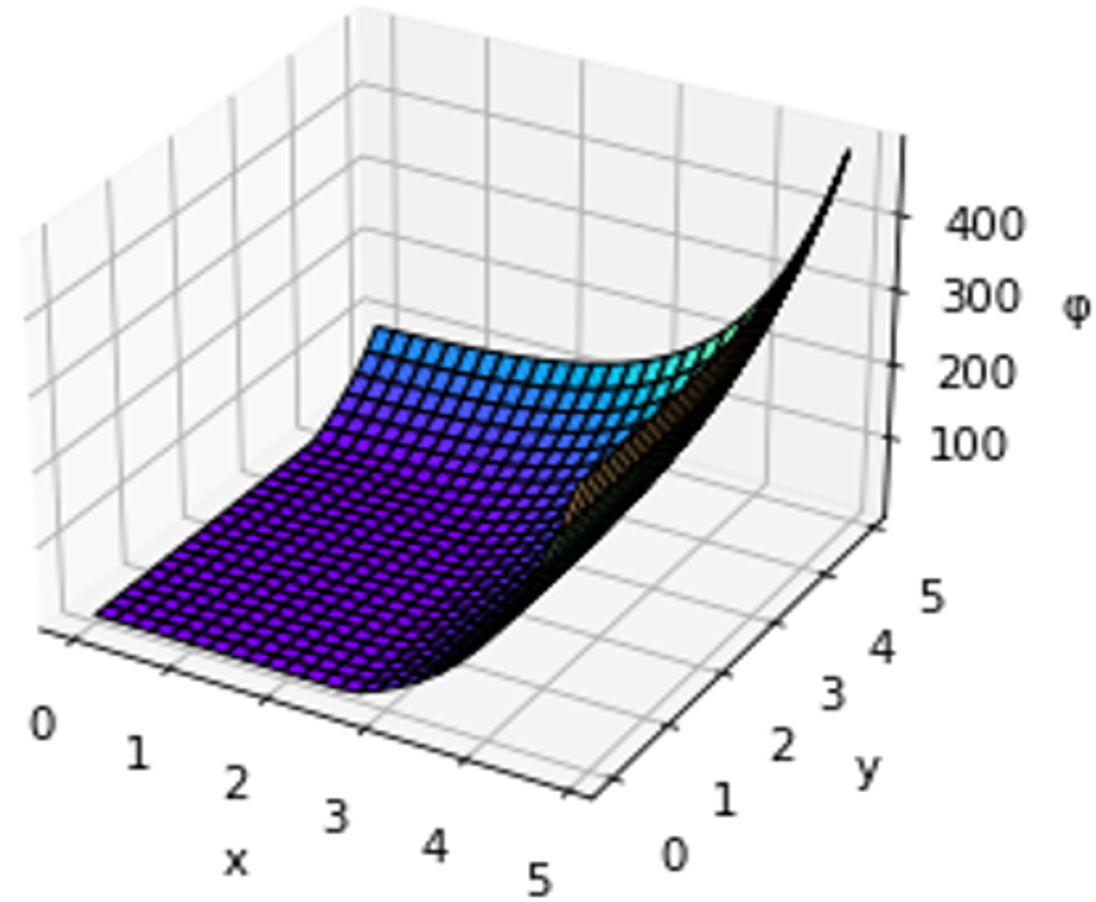
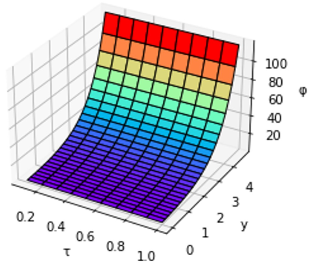
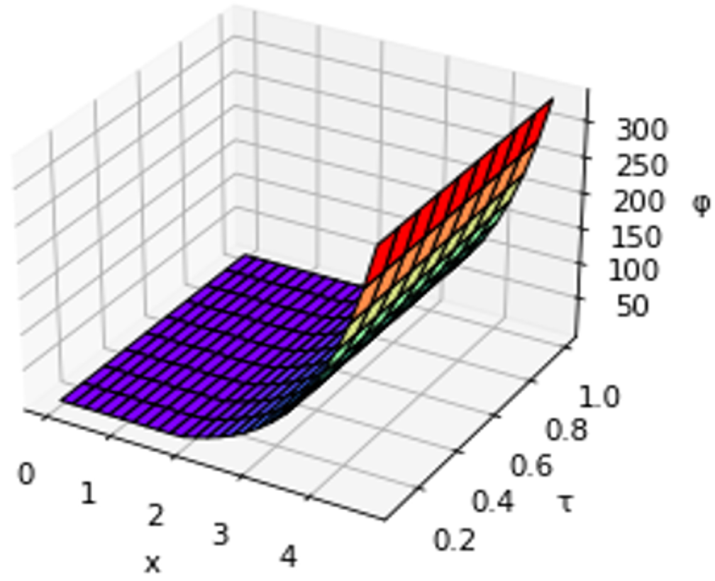
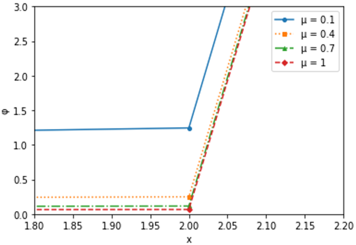
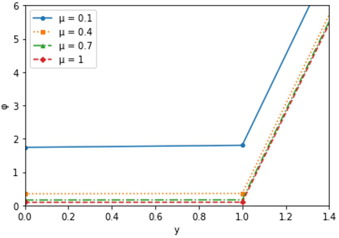
In this numerical illustration providing explicit solutions, we employ the parameters specified in Table 1 to calculate the solution for the European call option. Regarding the call option. Figures 1-5 illustrate plots of the modified explicit solution across various parameters. Figure 1 exhibits solutions ranging from 0 to 5 for $x$ and $y$. Figure 2 showcases the surface plot of the call option with $x=2.7080$ and time $0 \leq \tau \leq$ 1. The solution $\phi$ increases exponentially when $y$ is greater than 0 . Figure 3 presents the surface plot of the call option with $y=2.7080$ and time $0 \leq \tau \leq 1$. The solution $\phi$ grows exponentially when $x$ exceeds 2 . Within different orders of $\mu$ in the context of $\phi$, the values depicted in Figure 4 are $y=3.091$, and in Figure $5, x=3.555$. Through numerical simulations of Eq. (38), it is clear that the Laplace transform homotopy perturbation method [16], the ADM [18], the Generalized LHPM [20], all emerge as special cases of the CSHAM when the nonzero convergence-control parameter $h=-1$. Consequently, the CSHAM can be viewed as an enhancement of these existing methods.
Table 1. Parameters of the numerical solution
|
Parameters |
Values |
|
Strike price (K) |
45 |
|
Risk free interest rate (r) |
5% |
|
Expiration date (T) (Month) |
6 |
|
Volatility of underlying asset ($\zeta_1$) |
5% |
|
Volatility of underlying asset ($\zeta_2$) |
10% |
|
The volatility $S_1$ and $S_2$ ($\omega$) |
1 |
|
$\eta_1, \eta_2$ |
3, 2 |
Figure 1. The solution of $\phi$ when $x, y \in(0,5)$
Figure 2. The solution of $\phi$ for $\tau=0$ to 1 with $x=2.7080$
Figure 3. The solution of $\phi$ for $\tau=0$ to 1 with $x=3.21$
Figure 4. The solution of $\phi$ for various fractional-order values $y=3.091$
Figure 5. The solution of $\phi$ for various fractional-order values $x=3.555$
In our study, we successfully applied the conformable Shehu homotopy analysis technique to solve the two-dimensional B–S equation for a European call option. Compared to existing methodologies for solving the two-dimensional fractional Black-Scholes equation, the CSHAM decreases computational size, eliminates round-off errors, and ensures rapid convergence of series solutions within a few iterations, aided by the nonzero convergence-control parameter. The CSHAM, characterized by its simplicity, accuracy, adaptability, and efficiency, demonstrates significant advantages. Moreover, it is feasible to extend the application of the CSHAM to various types of ordinary and partial differential equations of non-integer order. Our future objective is to broaden the utilization of the CSHAM to address other systems of fractional ordinary differential equations (FODEs) encountered across different scientific domains.
[1] Black, F., Scholes, M. (1973). The pricing of options and corporate liabilities. Journal of Political Economy, 81(3): 637-654. https://doi.org/10.1086/260062
[2] Manale, J.M., Mahomed, F.M. (2000). A simple formula for valuing American and European call and put options. In Proceeding of the Hanno Rund Workshop on the Differential Equations, University of Natal.
[3] Merton, R.C. (1973). Theory of rational option pricing. The Bell Journal of Economics and Management Science, 4(1): 141-183.
[4] Cen, Z., Le, A. (2011). A robust and accurate finite difference method for a generalized Black–Scholes equation. Journal of Computational and Applied Mathematics, 235(13): 3728-3733. https://doi.org/10.1016/j.cam.2011.01.018
[5] Fabiao, F., Grossinho, M.D.R., Simões, O.A. (2009). Positive solutions of a Dirichlet problem for a stationary nonlinear Black–Scholes equation. Nonlinear Analysis: Theory, Methods & Applications, 71(10): 4624-4631. https://doi.org/10.1016/j.na.2009.03.026
[6] Fadugba, S.E. (2020). Homotopy analysis method and its applications in the valuation of European call options with time-fractional Black-Scholes equation. Chaos, Solitons & Fractals, 141: 110351. https://doi.org/10.1016/j.chaos.2020.110351
[7] Ouafoudi, M., Gao, F. (2018). Exact solution of fractional Black-Scholes European option pricing equations. Applied Mathematics, 9(1): 86-100. https://doi.org/10.4236/am.2018.91006
[8] Saratha, S.R., Sai Sundara Krishnan, G., Bagyalakshmi, M., Lim, C.P. (2020). Solving Black–Scholes equations using fractional generalized homotopy analysis method. Computational and Applied Mathematics, 39: 1-35. http://doi.org/10.1007/s40314-020-01306-4
[9] Vijayan, C., Manimaran, R. (2023). Application of homotopy analysis Shehu transform method for Fractional Black-Scholes equation. IAENG International Journal of Applied Mathematics, 53(2): 1-9.
[10] Khalil, R., Al Horani, M., Yousef, A., Sababheh, M. (2014). A new definition of fractional derivative. Journal of Computational and Applied Mathematics, 264: 65-70. https://doi.org/10.1016/j.cam.2014.01.002
[11] Abdeljawad, T. (2015). On conformable fractional calculus. Journal of Computational and Applied Mathematics, 279: 57-66. https://doi.org/10.1016/j.cam.2014.10.016
[12] Acan, O., Firat, O., Keskin, Y., Oturanc, G. (2016). Solution of conformable fractional partial differential equations by reduced differential transform method. Selcuk Journal of Applied Mathematics.
[13] Avcı, D., Eroglu, B.I., Ozdemir, N. (2016). Conformable heat problem in a cylinder. In International Conference on Fractional Differentiation and its Applications, Novi Sad, Serbia, pp. 572-581.
[14] Avcı, D., Iskender Eroğlu, B.B., Ozdemir, N. (2017). Conformable fractional wave-like equation on a radial symmetric plate. In Theory and Applications of Non-integer Order Systems: 8th Conference on Non-integer Order Calculus and Its Applications, Zakopane, Poland, pp. 137-146. https://doi.org/10.1007/978-3-319-45474-0-13
[15] Yavuz, M., Ozdemir, N. (2018). A different approach to the European option pricing model with new fractional operator. Mathematical Modelling of Natural Phenomena, 13(1): 12. https://doi.org/10.1051/mmnp/2018009
[16] Trachoo, K., Sawangtong, W., Sawangtong, P. (2017). Laplace transform homotopy perturbation method for the two dimensional Black Scholes model with European call option. Mathematical and Computational Applications, 22(1): 23. https://doi.org/10.3390/mca22010023
[17] Sawangtong, P., Trachoo, K., Sawangtong, W., Wiwattanapataphee, B. (2018). The analytical solution for the Black-Scholes equation with two assets in the Liouville-Caputo fractional derivative sense. Mathematics, 6(8): 129. https://doi.org/10.3390/math6080129
[18] Alfaqeih, S., Ozis, T. (2019). Solution of Black-Scholes fractional partial differential equation with two assets by Aboodh decomposition method. Progress in Fractional Differentiation and Applications, 6(4): 273-282. http://doi.org/10.18576/pfda/060404
[19] Prathumwan, D., Trachoo, K. (2020). On the solution of two-dimensional fractional Black–Scholes equation for European put option. Advances in Difference Equations, 2020(1): 146. https://doi.org/10.1186/s13662-020-02554-8
[20] Thanompolkrang, S., Sawangtong, W., Sawangtong, P. (2021). Application of the generalized Laplace homotopy perturbation method to the time-fractional Black–Scholes equations based on the Katugampola fractional derivative in Caputo type. Computation, 9(3): 33. https://doi.org/10.3390/computation9030033
[21] Benattıa, M.E., Belghaba, K. (2021). Shehu conformable fractional transform, theories and applications. Cankaya University Journal of Science and Engineering, 18(1): 24-32.
[22] Liaqat, M.I., Khan, A., Alqudah, M.A., Abdeljawad, T. (2023). Adapted homotopy perturbation method with Shehu transform for solving conformable fractional nonlinear partial differential equations. Fractals, 31(2).
[23] Jafari, H., Seifi, S. (2009). Homotopy analysis method for solving linear and nonlinear fractional diffusion-wave equation. Communications in Nonlinear Science and Numerical Simulation, 14(5): 2006-2012. https://doi.org/10.1016/j.cnsns.2008.05.008
[24] Bataineh, A.S., Noorani, M.S.M., Hashim, I. (2007). Solutions of time-dependent Emden–Fowler type equations by homotopy analysis method. Physics Letters A, 371(1-2).
[25] Unal, E., Gökdoğan, A. (2017). Solution of conformable fractional ordinary differential equations via differential transform method. Optik, 128: 264-273. http://doi.org/10.1016/j.ijleo.2016.10.031
[26] Maitama, S., Zhao, W. (2019). New integral transform: Shehu transform a generalization of Sumudu and Laplace transform for solving differential equations. International Journal of Analysis and Applications, 17(2): 167-190. https://doi.org/10.28924/2291-8639-17-2019-167
[27] Maitama, S., Zhao, W. (2019). Local fractional Laplace homotopy analysis method for solving non-differentiable wave equations on Cantor sets. Computational and Applied Mathematics, 38: 65. http://doi.org/10.1007/s40314-019-0825-5
[28] Babolian, E., Azizi, A., Saeidian, J. (2009). Some notes on using the homotopy perturbation method for solving time-dependent differential equations. Mathematical and Computer Modelling, 50(1-2): 213-224. https://doi.org/10.1016/j.mcm.2009.03.003