Menaka Muthuramu![]() | Manimaran Rajendran*
| Manimaran Rajendran*![]() | Jeyabarathi Ponraj
| Jeyabarathi Ponraj![]() | Rajendran Lakshmanan
| Rajendran Lakshmanan![]()
© 2024 The authors. This article is published by IIETA and is licensed under the CC BY 4.0 license (http://creativecommons.org/licenses/by/4.0/).
OPEN ACCESS
Nonlinear differential equations often arise in many real-world problems. The complexity of solving nonlinear systems arises from the strong interdependence between the variables of the system and the boundary conditions. An immobilized glucose isomerase-based mathematical model for the enzymatic isomerization process that converts glucose to fructose is presented. The model's kinetic mechanism is stated using the nonlinear reaction-diffusion equation for MichalisMenten kinetics. The general approximate analytical formulas for the glucose molar concentration and flux inside packed-bed reactors are determined by solving the nonlinear equation using Akbari-Ganji's method. The effects of the kinetic parameters and pore-level Thiele modulus on concentration and flux were discussed. Estimating the kinetic parameters from current density is suggested. It has been shown that this method reduces processing time without affecting the quality of the solution. This method works well for many different types of nonlinear systems, making it useful in engineering and other fields of science.
reaction-diffusion, mathematical modelling and numerical simulation, Akbari-Ganji method, glucose isomerase
In biochemistry, a large class of enzymes known as isomerases is responsible for changing a molecule's isomer. Enzyme-based isomer formation is a widely used technique for transforming glucose to fructose. This procedure, which takes place in a packed-bed reactor containing microporous materials with various particle diameters, uses immobilized glucose isomerase. By employing enzymatic isomerization to produce glucose in economically viable quantities, Marshall and Kooi [1] developed glucose isomerase.
One of the more effective methods is the isomeric formation of sugar to fructose by immobilized glucose isomerase. It is done in fixed-bed and fluidized-bed reactors, as well as continuous stirred-tank reactors, in addition to batch reactors.
In the latter two scenarios, a significant surface area is provided for the reactions by the holes of the porous nanoparticles which immobilizes the enzymes. Packet-bed reactors are extensively employed because it is simple to assemble a packing of microporous particles. As a result, there has been a lot of focus on the difficulty of simulating the enzymatic conversion of glucose to fructose in packed-bed reactors. The models were constructed to forecast the effectiveness of packed-bed reactors in this process.
The effects of heterogeneities on mass transport and reaction characteristics in porous media are quantitatively described by percolation theory [2-9]. Numerous people have modelled the deactivation of catalysts at only one porous particle using this methodology [10-16]. Dadvar and co-workers presented a three-dimensional particle-level [17] and Monte-Carlo computer simulations [18] of the Pore network theory of this process in packed-bed reactors [19].
Margret Ponrani and Rajendran [20] applied the homotopy perturbation method to solve the glucose isomerase's non-linear equation. However, the concentration and current generated by this approach have a lengthy-expression. Ananthasamy et al. [21] provided theoretical result for concentration and flux at a planar microelectrode using a new homotopy approach. However, the error differences between the analytical and numerical solutions in this method increase for large parameter values. Using an analytical approach based on wavelets, Selvi and Hariharan [22] determined the steady-state concentration. The drawbacks of this approach are the implementation difficulty and the wavelet's dependence on boundary conditions.
At present, there are no simple theoretical results available for the steady-state glucose concentration and current for all values of the variables such as $C_{z 0}, C_{z 1}, \Phi_p$ and $\beta$. This manuscript aims to apply Akbari-Ganji's (AGM) approach to establish an analytical formula for the steady-state current and substrate concentration. Our theoretical expression of current predicts the kinetics parameters in packed-bed reactors, which are used to improve operational control and reactor design flexibility. AGM's main advantage is obtaining a solution by simple basic computations. These approaches are effective for both weak and strong nonlinear systems.
The reaction kinetics of the glucose enzyme are expressed as follows [17]:
$G+E \leftrightharpoons_{k_{-1}}^{k_1} X \leftrightharpoons_{k_{-2}}^{k_2} F+E$ (1)
where, G, E, and F are the glucose, fructose, and enzyme, respectively, and X denotes the intermediate complex that is produced. $k_1, k_2$ and $k_{-1}, k_{-2}$ are kinetic rate constants. Assuming the existence of a pseudo-steady state, one must
$\frac{d X}{d t}=k_1 E G-\left(k_{-1}+k_2\right) X+k_{-2} E F \simeq 0$ (2)
The following variables are introduced:
$R=\frac{{{v}_{m}}~\bar{G}}{{{K}_{m}}+\bar{G}},{{v}_{m}}=\frac{{{K}_{mr}}{{v}_{mr}}\left( 1+{{K}^{-1}} \right)}{{{K}_{mr}}-{{K}_{mf}}},{{K}_{m}}=\frac{{{K}_{mf~}}{{K}_{mr}}\left[ 1+\left( K_{mf}^{-1}+KK_{mf}^{-1} \right){{G}_{0}}{{\left( 1+K \right)}^{-1}} \right]}{{{K}_{mr-{{K}_{mf}}}}}$ (3)
The mass balance equation is written as [17]:
$D_p(\lambda) \frac{d^2 G}{d z^2}-\frac{2}{r a} R=0$ (4)
where, $\lambda=\frac{R_M}{r}=\frac{\text { molecular radius }}{\text { pore radius }}$. The other parameters have the usual meaning [17]. Diffusion is the primary mass transfer process in the particle's pore region since the pores are usually tiny. We presume that steady-state conditions exist. Only changes in G in axial direction z are essential, as our main focus is on the macroscopic mass transfer process. At the network's nodes, we further assume no chemical processes or adsorption are occurring in place. Eq. (4) may be rewritten as follows:
$D_p \frac{d^2 \bar{G}}{d z^2}-\frac{2}{r a} \frac{V_m \bar{G}}{\left(K_m+\bar{G}\right)}=0$ (5)
The following dimensionless variables are introduced,
$\begin{aligned} & C=\frac{\bar{G}}{\left(G_0-G_e\right)}, z=\frac{x}{l}, \beta=\frac{\overline{C_0}}{K_m}, \Phi_p^2=\frac{2 l^2 V_m^{\prime}}{r D_p K_m}, V_m^{\prime} =\frac{V_m}{a}\end{aligned}$ (6)
where, $\Phi_p$ represents the pore-level Thiele modulus, l denotes the pore length. Eq. (6) is reduced to the dimensionless form as follows:
$\frac{d^2 C(z)}{d z^2}-\Phi_p^2 \frac{C(z)}{1+\beta C(z)}=0$ (7)
The Thiele modulus $\Phi_p^2$ is invented to characterise the relation between diffusion and reaction rates without mass transfer constraints. This measurement is commonly applied to determine the efficacy factor of pellets. Smaller values of the $\Phi_p^2$ represent slow reactions with fast diffusion. Large values indicate rapid reactions with slower diffusion. The value $\Phi_p^2$ is related to pore length, pore radius, maximum reaction rate, diffusion coefficient and Michaelin-Menten constant. $\beta$ is the saturation parameter. Since it reflects the ratio of substrate concentration and the Michaelin-Menten constant, this parameter quantifies the level of saturation or unsaturation of the catalytic processes. The dimensionless boundary conditions are:
$C(z=0)=C_{z 0}$ (8)
$C(z=1)=C_{z 1}$ (9)
Then, the dimensionless current can be calculated using:
$J_{i j}=\left(\frac{d c}{d z}\right)_{z=1}$ (10)
Asymptotic methods for solving many nonlinear equations in the mathematical sciences include variation iteration [23, 24], Padé approximation [25, 26], Akbari-Ganji's [27-30], homotopy perturbation [31, 32], new homotopy perturbation [33, 34], Adomian decomposition [35], and Taylor series [36, 37] methods. Taylor's series and the Akbari-Ganij method are the simplest techniques when the domain of the problem is finite. However, the Rajendran-Joy method [38, 39] may be applied in finite and semi-infinite regions.
Compared to other approaches, AGM yields adequate precision and accuracy and is fairly near the exact solution of the equation. This approach states that our trial function for the required solution comprises three constants that have been determined by a series of simple algebraic computations [40]. On the other hand, the other approaches have complicated procedures to arrive the result. Applying this technique, we derive the following analytical equation for substrate concentration (Appendix A):
$C(z)=C_{z 0}+\left(C_{z 1}-C_{z 0}\right) z+\frac{\Phi_p^2 C_{z 1}}{2\left(1+\beta C_{z 1}\right)}\left(z^2-z\right)$ (11)
Now, from Eq. (11), the normalized current is given by:
$J_{i j}=C_{z 1}-C_{z 0}+\frac{\Phi_p^2 C_{z 1}}{2\left(1+\beta C_{z 1}\right)}$ (12)
3.1 Previous analytical results
The new homotopy perturbation method (NHPM) was employed by Ananthaswamy et al. [21] to solve the Eq. (7). They determined the normalised substrate concentration as follows:
$C(z)=\frac{C_{z 0} \sinh \left(\frac{\Phi_p(1-z)}{\sqrt{1+\beta} C_{z 0}}\right)+C_{z 1} \sinh \left(\frac{\Phi_p z}{\sqrt{1+\beta} C_{z 0}}\right)}{\sinh \left(\frac{\Phi_p}{\sqrt{1+\beta} C_{z 0}}\right)}$ (13)
The normalized current is given by:
$J_{i j}=\frac{\boldsymbol{\Phi}_p}{\sqrt{1+\beta C_{z 0}}}\left[\frac{C_{z 1} \cosh \left(\frac{\Phi_p}{\sqrt{1+\beta C_{z 0}}}\right)-C_{z 0}}{\sinh \left(\frac{\Phi_p}{\sqrt{1+\beta C_{z 0}}}\right)}\right]$ (14)
The numerical data verify our new analytical results. We have solved the initial boundary value problems numerically using SCILAB/ MATLAB software's function pdex1. For different values of the $\beta$ and $\Phi_p$, our analytical findings were validated with simulation data and earlier analytical results (NHPM) in Tables 1 to 3. Our new AGM-based analytical methods have a maximum average error of 15% with simulation results.
Table 1. A comparison of the concentration of substrate C(z) for different variables $\Phi_p$ using numerical and analytical methods when $\beta=1, C_{z 0}=C_{z 1}=2$
|
z |
$\boldsymbol{\Phi}_p=\mathbf{1}$ |
$\boldsymbol{\Phi}_p=\mathbf{1.5}$ |
$\boldsymbol{\Phi}_p=\mathbf{2}$ |
||||||||||||
|
|
Num. |
Concentration |
Error (%) |
Num. |
Concentration |
Error (%) |
Num. |
Concentration |
Error (%) |
||||||
|
This Work AGM Eq. (11) |
NHPM [21] Eq. (13) |
This Work AGM Eq. (11) |
NHPM [21] Eq. (13) |
This Work AGM Eq. (11) |
NHPM [21] Eq. (13) |
This Work AGM Eq. (11) |
NHPM [21] Eq. (13) |
This Work AGM Eq. (11) |
NHPM [21] Eq. (13) |
This Work AGM Eq. (11) |
NHPM [21] Eq. (13) |
||||
|
0 |
2.0000 |
2.0000 |
2.0000 |
0.0000 |
0.0000 |
2.0000 |
2.0000 |
2.0000 |
0.0000 |
0.0000 |
2.0000 |
2.0000 |
2.0000 |
0.0000 |
0.0000 |
|
0.2 |
1.9470 |
1.9460 |
1.9480 |
0.0510 |
0.0514 |
1.8820 |
1.8790 |
1.8870 |
0.1594 |
0.2657 |
1.7950 |
1.7850 |
1.8100 |
0.5571 |
0.8356 |
|
0.4 |
1.9210 |
1.9200 |
1.9220 |
0.0521 |
0.0521 |
1.8240 |
1.8190 |
1.8320 |
0.2741 |
0.4386 |
1.6940 |
1.6790 |
1.7180 |
0.8855 |
1.4168 |
|
0.6 |
1.9210 |
1.9200 |
1.9230 |
0.0521 |
0.0542 |
1.8260 |
1.8210 |
1.8340 |
0.2738 |
0.4381 |
1.6970 |
1.6820 |
1.7200 |
0.8839 |
1.3553 |
|
0.8 |
1.9490 |
1.9480 |
1.9500 |
0.0513 |
0.0513 |
1.8870 |
1.8840 |
1.8910 |
0.1590 |
0.2120 |
1.8020 |
1.7930 |
1.8170 |
0.4994 |
0.8324 |
|
1 |
2.0000 |
2.0000 |
2.0000 |
0.0000 |
0.0000 |
2.0000 |
2.0000 |
2.0000 |
0.0000 |
0.0000 |
2.0000 |
2.0000 |
2.0000 |
0.0000 |
0.0000 |
|
|
Average error (%) |
0.0348 |
0.0349 |
Average error (%) |
0.1444 |
0.2257 |
Average error (%) |
0.4710 |
0.7400 |
||||||
Table 2. A comparison of the concentration of substrate C(z) for different variables $\Phi_p$ using numerical and analytical methods when $\beta=5, C_{z 0}=3, C_{z 1}=4$
|
z |
$\boldsymbol{\Phi}_p=\mathbf{1}$ |
$\boldsymbol{\Phi}_p=\mathbf{3}$ |
$\boldsymbol{\Phi}_p=\mathbf{9}$ |
||||||||||||
|
|
Num. |
Concentration |
Error (%) |
Num. |
Concentration |
Error (%) |
Num. |
Concentration |
Error (%) |
||||||
|
This Work AGM Eq. (11) |
NHPM [21] Eq. (13) |
This Work AGM Eq. (11) |
NHPM [21] Eq. (13) |
This Work AGM Eq. (11) |
NHPM [21] Eq. (13) |
This Work AGM Eq. (11) |
NHPM [21] Eq. (13) |
This Work AGM Eq. (11) |
NHPM [21] Eq. (13) |
This Work AGM Eq. (11) |
NHPM [21] Eq. (13) |
||||
|
0 |
3.0000 |
3.0000 |
3.0000 |
0.0000 |
0.0000 |
3.0000 |
3.0000 |
3.0000 |
0.0000 |
0.0000 |
3.0000 |
3.0000 |
3.0000 |
0.0000 |
0.0000 |
|
0.2 |
3.1870 |
3.1870 |
3.1850 |
0.0000 |
0.0627 |
3.0650 |
3.0640 |
3.0560 |
0.0326 |
0.2936 |
2.0190 |
1.9580 |
2.2740 |
3.0213 |
1.2630 |
|
0.4 |
3.3810 |
3.3810 |
3.3780 |
0.0000 |
0.0887 |
3.2000 |
3.1980 |
3.1820 |
0.0625 |
0.5625 |
1.6400 |
1.5470 |
2.0250 |
5.6707 |
23.476 |
|
0.6 |
3.5830 |
3.5830 |
3.5800 |
0.0000 |
0.0837 |
3.4030 |
3.4010 |
3.3820 |
0.0588 |
0.0587 |
1.8520 |
1.7640 |
2.2020 |
4.7516 |
18.898 |
|
0.8 |
3.7930 |
3.7930 |
3.7910 |
0.0000 |
0.0527 |
3.6760 |
3.6750 |
3.6590 |
0.0272 |
0.0272 |
2.6620 |
2.6120 |
2.8420 |
1.8783 |
6.7618 |
|
1 |
4.0000 |
4.0000 |
4.0000 |
0.0000 |
0.0000 |
4.0000 |
4.0000 |
4.0000 |
0.0000 |
0.0000 |
4.0000 |
4.0000 |
4.0000 |
0.0000 |
0.0000 |
|
|
Average error (%) |
0.0000 |
0.0480 |
Average error (%) |
0.0257 |
0.1570 |
Average error (%) |
2.5536 |
8.3998 |
||||||
Table 3. A comparison of the concentration of substrate C(z) for different variables $\Phi_p$ using numerical and analytical methods when $\beta=10, C_{z 0}=5, C_{z 1}=5$
|
z |
$\boldsymbol{\Phi}_p=\mathbf{5}$ |
$\boldsymbol{\Phi}_p=\mathbf{10}$ |
$\boldsymbol{\Phi}_p=\mathbf{15}$ |
||||||||||||
|
|
Num. |
Concentration |
Error (%) |
Num. |
Concentration |
Error (%) |
Num. |
Concentration |
Error (%) |
||||||
|
This Work AGM Eq. (11) |
NHPM [21] Eq. (13) |
This Work AGM Eq. (11) |
NHPM [21] Eq. (13) |
This Work AGM Eq. (11) |
NHPM [21] Eq. (13) |
This Work AGM Eq. (11) |
NHPM [21] Eq. (13) |
This Work AGM Eq. (11) |
NHPM [21] Eq. (13) |
This Work AGM Eq. (11) |
NHPM [21] Eq. (13) |
||||
|
0 |
5.0000 |
5.0000 |
5.0000 |
0.0000 |
0.0000 |
5.0000 |
5.0000 |
5.0000 |
0.0000 |
0.0000 |
5.0000 |
5.0000 |
5.0000 |
0.0000 |
0.0000 |
|
0.2 |
4.8030 |
4.8020 |
4.8110 |
0.0208 |
0.1667 |
4.2130 |
4.2100 |
4.3350 |
0.0712 |
2.8958 |
3.2490 |
3.2220 |
3.7480 |
0.8310 |
15.359 |
|
0.4 |
4.7050 |
4.7050 |
4.7190 |
0.0000 |
0.2997 |
3.8260 |
3.8200 |
4.0190 |
0.1568 |
5.0444 |
2.3890 |
2.3440 |
3.1810 |
1.8836 |
33.152 |
|
0.6 |
4.7080 |
4.7070 |
4.7220 |
0.0212 |
0.2974 |
3.8360 |
3.8300 |
4.0270 |
0.1564 |
4.9791 |
2.4110 |
2.3670 |
3.1950 |
1.8250 |
32.518 |
|
0.8 |
4.8100 |
4.8100 |
4.8180 |
0.0000 |
0.1663 |
4.2430 |
4.2400 |
4.3600 |
0.0707 |
2.7575 |
3.3150 |
3.2890 |
3.7930 |
0.7843 |
14.420 |
|
1 |
5.0000 |
5.0000 |
5.0000 |
0.0000 |
0.0000 |
5.0000 |
5.0000 |
5.0000 |
0.0000 |
0.0000 |
5.0000 |
5.0000 |
5.0000 |
0.0000 |
0.0000 |
|
|
Average error (%) |
0.0070 |
0.1550 |
Average error (%) |
0.0758 |
2.6128 |
Average error (%) |
0.8873 |
15.918 |
||||||
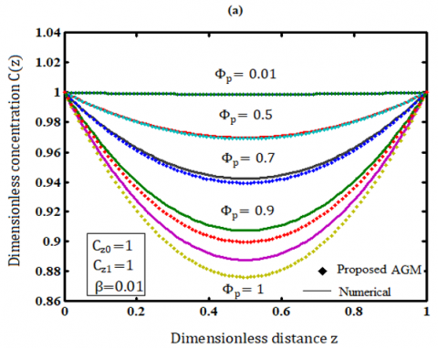
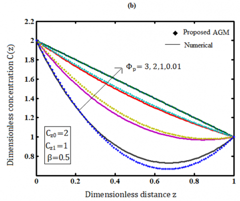
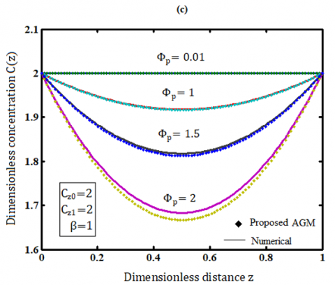
The simple approximate analytical result of substrate concentration is represented by Eq. (11) for all parameter values. The new primary analytical flux expression is found in Eq. (12). The values of the parameters $C_{z 0}, C_{z 1}, \Phi_p$ and $\beta$ determine the substrate concentration. The ratio of the square of pore length to pore radius ($\frac{l^2}{r}$) influences the Thiele modulus. This value shows the significance of diffusion and reaction in the deposited surface. Also from the Eq. (11), the concentration of glucose is minimum when
$z=\frac{-C_1}{2 C_2}=\frac{\left(1+\beta C_{z 1}\right)}{\Phi_p^2 C_{z 1}}\left[C_{z 0}+\frac{\Phi_p^2 C_{z 1}}{2\left(1+\beta C_{z 1}\right)}-C_{z 1}\right]$ (15)
The minimum value is
$\begin{gathered}C(z)_{\min }=C_{z 0}-\frac{C_1^2}{4 C_2}=C_{z 0}-\frac{\left(1+\beta C_{z 1}\right)}{2 \Phi_p^2 C_{z 1}}\left[C_{z 1}-C_{z 0}-\frac{\Phi_p^2 C_{z 1}}{2\left(1+\beta C_{z 1}\right)}\right]^2\end{gathered}$ (16)
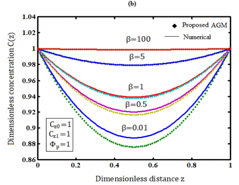
When $C_{z 1}=C_{z 0}$ the concentration of glucose is minimum at z=0.5 and have the minimum value:
$C(z)_{\min }=C_{z 0}-\frac{\Phi_p^2 C_{z 0}}{8\left(1+\beta C_{z 0}\right)}$ (17)
These results are also conformed in Figure 1.
Figure 1. The impact of the parameters $\Phi_p, C_{z 1}$ and $C_{z 0}$ on concentration of glucose. Solid line: Numerical result; dashed-dotted line: Eq. (11)
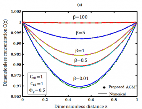
Figure 2. The impact of the kinetic parameter $\beta$ on the glucose concentration. Solid line: Numerical result; dashed-dotted line: Eq. (11)
Changes in pore length and pore radius can alter the parameter $\Phi_p$. This variable illustrates the significance of reaction and diffusion in the layer of enzymes.
The concentration of glucose C is shown in Figures 1 and 2 for different values of the parameter $\beta$ and $\Phi_p$. It is clear from the data that when z=1, the glucose concentration attains its maximum value of 1. Figure 1 illustrates the glucose concentration for a range of $\Phi_p$ values. From the Figure, it is inferred that the concentration of glucose is decreases when pore-level Thiele modulus $\Phi_p$ rises. Additionally, the concentration is constant when $\Phi_p \ll 0.01$ for every value of the other parameters. But the maximum or minimum value of the concentration of glucose at z=1 is depending upon the value of $C_{z 1}$ and $C_{z 0}$ (Figure 2).
The concentration of glucose for various values of the dimensionless kinetic parameter $\beta$ is shown in Figure 2. A positive correlation can be observed in Figure 2 between the corresponding substrate concentration and the dimensionless kinetic parameter $\beta$.
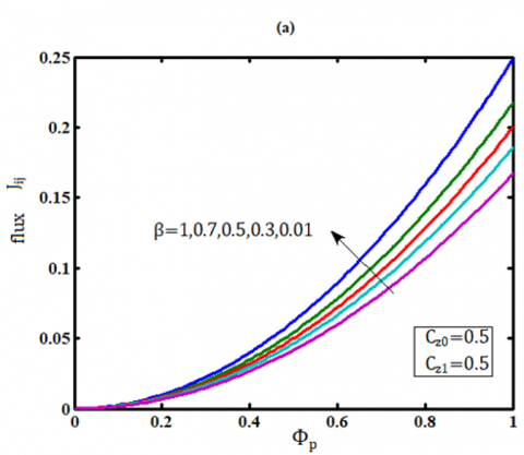
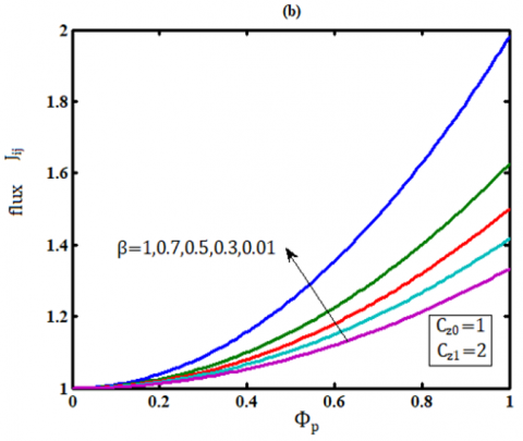
Figure 3. The influence of variables $\Phi_p, \beta, C_{z 0}$, and $C_{z 1}$ on the flux $J_{i j}$ using Eq. (12)
The dimensionless flux $J_{i j}$ vs. the dimensionless kinetic parameter $\beta$ is depicted in Figure 3 for a various of Thiele modulus values. As the parameters $\beta$ and $\Phi_p$ decrease, the flux value increases, as seen in this figure.
The sensitivity analysis ascertains the effect of every variable on the current. Their impact on the current can be identified by analysing the current slope about the appropriate parameters. The steady-state current's sensitivity analysis is shown in Figure 4. Regarding the parameters $C_{z 0}, C_{z 1}, \Phi_p$ and $\beta$ the percentage change in current is 42, 47, 10, and 1, respectively. From the figures, it is inferred that the current density appears to be more strongly influenced by the concentration at the boundaries ($C_{z 0}$ and $C_{z 1}$), than by the Thiele modulus and rate constant.
Figure 4. Analysing the parameters' sensitivity to current density when $C_{z 1}=0.5, \Phi_p=0.6$ and $\beta=0.5$
The Eq. (12) can be written as follows:
$\frac{1}{2\left(J_{i j}-C_{z 1}+C_{z 0}\right)}=\frac{1}{\Phi_p^2 C_{z 1}}+\frac{\beta}{\Phi_p^2}$ (18)
The value of $J_{i j}$ can be experimentally evaluated for different values of concentration $C_{Z 1}$. Note that the given equation follows the general pattern of a straight line $(y=m x+c)$. The plot of $\frac{1}{2\left(J_{i j}-C_{z 1}+C_{z 0}\right)}$ versus $\frac{1}{C_{z 1}}$ gives the slope $\frac{1}{\Phi_p^2}$ and intercept $\frac{\beta}{\Phi_p^2}$. From the slope and intercept, we can obtain the value of Theile modulus $\left(\Phi_p^2\right)$ (which is directly related to the ratio of the square of pore length and pore radius $\left(l^2 / r\right)$ and kinetic parameter $(\beta)$. Our analytical expression of current predicts the kinetics parameters in packed-bed reactors, which is used to optimise the operational control and reactor design flexibility.
The reaction and kinetics of immobilised glucose isomerase in packed bed reactors with the Michaelis-Menten scheme have been discussed. A closed-form equation for glucose concentration and flux in the packed-bed reactor at a planar microelectrode is obtained using Akbari-Ganji’s method. Additionally, the impact of different parameters on the flux is studied. This theoretical technique can be readily extended to solve all nonlinear equations for diverse, complex boundary conditions in different kinetics schemes, including competitive and non-competitive inhibitors, Briggs Haldane and non-Michaelis-Menten kinetics. This approach may also solve nonlinear problems in biosensors and biofuel cells.
Approximate analytical solution nonlinear Eq. (7) using AGM method.
We may assume that the initial solution of Eq. (7) is
$C(z)=\sum_{i=0}^2 C_i z^i=C_0+C_1 z+C_2 z^2$ (A1)
where, $C_0, C_1$ and $C_2$ are unknown constants. Applying the boundary conditions (8) and (9), we obtain:
$C_0=C_{z0}, \quad C_1+C_2=C_{z1}-C_{{z } 0}$ (A2)
Hence the Eq. (A1) becomes:
$C(z)=C_{z 0}+\left(C_{z 1}-C_{z 0}-C_2\right) z+C_2 z^2$ (A3)
The only unknown constant, C2, may be determined using the AGM approach as follows:
Now define the function H by:
$H(z): \frac{d^2 C(z)}{d z^2}-\frac{\Phi_p^2 C(z)}{1+\beta C(z)} 0$, (A4)
Using the Eq. (A3), the Eq. (A4) becomes:
$H(z): 2 C_2-\frac{\Phi_p^2 C(z)}{1+\beta C(z)}=0$ (A5)
At z=1, the previous equation yields:
$H(z=1): 2 C_2-\frac{\Phi_p^2 C_{z 1}}{1+\beta C_{z 1}}=0$ (A6)
Consequently, the constants C1 and C2 becomes:
$C_2=\frac{\Phi_p^2 C_{z 1}}{2\left(1+\beta C_{z 1}\right)}, C_1=C_{z 1}-C_{z 0}-\frac{\Phi_p^2 C_{z 1}}{2\left(1+\beta C_{z 1}\right)}$ (A7)
Now the Eq. (A3) becomes:
$\begin{aligned} & C(z)=C_{z 0}+\left(C_{z 1}-C_{z 0}\right) z+\frac{\Phi_p^2 C_{z 1}}{2\left(1+\beta C_{z 1}\right)}\left(z^2-z\right)\end{aligned}$ (A8)
Eq. (A8) provides a closed-form expression of glucose concentration C(z).
[1] Marshall, R.O., Kooi, E.R. (1957). Enzymatic conversion of D-glucose to D-fructose. Science, 125(3249): 648-649. https://doi.org/10.1126/science.125.3249.648
[2] Stauffer, D., Aharony, A. (1992). Introduction to Percolation Theory (2nd ed.). London: Taylor & Francis.
[3] Sahimi, M., Gavalas, G.R., Tsotsis, T.T. (1990). Statistical and continuum models of fluid-solid reactions in porous media. Chemical Engineering Science, 45(6): 1443-1502. https://doi:10.1016/0009-2509(90)80001-U
[4] Sahimi, M. (1992). Transport of macromolecules in porous media. Journal of Chemical Physics, 96: 4718. https://doi.org/10.1063/1.462782
[5] Sahimi, M. (1993). Flow phenomena in rocks: From continuum models to fractals, percolation, cellular automata, and simulated annealing. Reviews of Modern Physics, 65: 1393. https://doi.org/10.1103/RevModPhys.65.1393
[6] Sahimi, M. (1994). Applications of Percolation Theory. London: Taylor & Francis. https://doi.org/10.1201/9781482272444
[7] Sahimi, M. (1995). Flow and transport in porous media and fractured rock. Weinheim: VCH. 482.
[8] Sahimi, M. (2003). Heterogeneous Materials. Vols. I, II. New York: Springer. https://doi.org/10.1007/b97505
[9] Rieckmann, C., Keil, F.J. (1999). Simulation and experiment of multicomponent diffusion and reaction in three-dimensional networks. Chemical Engineering Science, 54(15-16): 3485-3493. https://doi.org/10.1016/S0009-2509(98)00480-1
[10] Beyne, A.O.E., Froment, G.F. (1990). A percolation approach for the modeling of deactivation of zeolite catalysts by coke formation. Chemical Engineering Science, 45(8): 2089-2096. https://doi.org/10.1016/0009-2509(90)80081-O
[11] Arbabi, S., Sahimi, M. (1991). Computer simulations of catalyst deactivation—I. Model formulation and validation. Chemical Engineering Science, 46(7): 1739-1747. https://doi.org/10.1016/0009-2509(91)87020-D
[12] Arbabi, S., Sahimi, M. (1991). Computer simulations of catalyst deactivation—II. The effect of morphological, transport and kinetics parameters on the performance of the catalyst. Chemical Engineering Science, 46(7): 1749-1755. https://doi.org/10.1016/0009-2509(91)87021-4
[13] Keil, F.J., Rieckmann, C. (1994). Optimization of three-dimensional catalyst pore structures. Chemical Engineering Science, 49(24): 4811-4822. https://doi.org/10.1016/S0009-2509(05)80061-2
[14] Zhang, L., Seaton, N.A. (1996). Simulation of catalyst fouling at the particle and reactor levels. Chemical Engineering Science, 51(12): 3257-3272. https://doi.org/10.1016/0009-2509(95)00388-6
[15] Rieckmann, C., Keil, F.J. (1997). Multicomponent diffusion and reaction in three-dimensional networks: General kinetics. Industrial & Engineering Chemistry Research, 36(8): 3275-3281. https://doi.org/10.1021/ie9605847
[16] Rieckmann, C., Keil, F.J. (1999). Simulation and experiment of multicomponent diffusion and reaction in three-dimensional networks. Chemical Engineering Science, 54(15-16): 3485-3493. https://doi.org/10.1016/S0009-2509(98)00480-1
[17] Dadvar, M., Sahimi, M. (2003). Pore network model of deactivation of immobilized glucose isomerase in packed-bed reactors. Part III: Multiscale modelling. Chemical Engineering Science, 58(22): 4935-4951. https://doi.org/10.1016/j.ces.2003.07.006
[18] Dadvar, M., Sahimi, M. (2002). Pore network model of deactivation of immobilized glucose isomerase in packed-bed reactors. II. Three-dimensional simulation at the particle level. Chemical Engineering Science, 57(6): 939-952. https://doi.org/10.1016/S0009-2509(02)00014-3
[19] Dadvar, M., Sohrabi, M., Sahimi, M. (2001). Pore network model of deactivation of immobilized glucose isomerase in packed-bed reactors. I. Two-dimensional simulation at the particle level. Chemical Engineering Science, 56(8): 2803-2819. https://doi.org/10.1016/S0009-2509(00)00548-0
[20] Margret Ponrani, V., Rajendran, L. (2012). Mathematical modelling of steady-state concentration in immobilized glucose isomerase of packed-bed reactors. Journal of Mathematical Chemistry, 50: 1333-1346. https://doi.org/10.1007/s10910-011-9973-6
[21] Ananthaswamy, V., Padmavathi, P., Rajendran, L. (2014). Simple analytical expressions of the steady state concentration and flux in immobilized glucose isomerase of packed-bed reactors. Review of Bioinformatics and Biometrics, 3: 29-37.
[22] Selvi, M.S.M., Hariharan, G. (2016). Wavelet-based analytical algorithm for solving steady-state concentration in the immobilized glucose isomerase of a packed-bed reactor model. Journal of Membrane Biology, 249(4): 559-568. https://doi.org/10.1007/s00232-016-9905-2
[23] He, J.H., Hong Wu, X. (2007). Variational iteration method: New development and applications. Computers & Mathematics with Applications, 54(7-8): 881-894. https://doi.org/10.1016/j.camwa.2006.12.083
[24] Wu, G.C., Baleanu, D. (2013). New applications of the variational iteration method from differential equations to q-fractional difference equations. Advances in Difference Equations, 21: 13-21. https://doi.org/10.1186/1687-1847-2013-21
[25] Andrianov, I., Shatrov, A. (2021). Padé approximants, their properties, and applications to hydrodynamic problems. Symmetry, 13(10): 1869. https://doi.org/10.3390/sym13101869
[26] Kalateh Bojdi, Z., Ahmadi-Asl, S., Aminataei, A. (2013). A new extended Padé approximation and its application. Advances in Numerical Analysis, Article ID: 263467. https://doi.org/10.1155/2013/263467
[27] Jeyabarathi, P., Rajendran, L., Lyons, M.E.G., Abukhaled, M. (2022). Theoretical analysis of mass transfer behavior in fixed-bed electrochemical reactors: Akbari-Ganji’s method. Electrochem, 3: 699-712. https://doi.org/10.3390/electrochem3040046
[28] Akbari, M.R., Ganji, D.D., Nimafar, M., Ahmadi, A.R. (2014). Significant progress in the solution of nonlinear equations at the displacement of structure and heat transfer extended surface by a new AGM approach. Frontiers of Mechanical and Engineering, 9(4): 390-401. https://doi.org/10.1007/s11465-014-0313-y
[29] Akbari, M. (2015). Nonlinear Dynamic in Engineering by Akbari-Ganji’s Method. Xlibris Corporation.
[30] Ganji, D.D., Talarposhti, R.A. (2017). Numerical and analytical solutions for solving nonlinear equations in heat transfer. Hershey, PA: IGI Global. https://doi.org/10.4018/978-1-5225-2713-8
[31] He, J.H., El-Dib, Y.O., Mady, A.A. (2021). Homotopy perturbation method for the fractal toda oscillator. Fractal and Fractional, 5(3): 93. https://doi.org/10.3390/fractalfract5030093
[32] He, J.H., El Dib, Y.O. (2021). Homotopy perturbation method with three expansions. Journal of Mathematical Chemistry, 59(4): 1139-1150. https://doi.org/10.1007/s10910-021-01237-3
[33] Biazar, J., Eslami, M. (2011). A new homotopy perturbation method for solving systems of partial differential equations. Computers & Mathematics with Applications, 62(1): 225-234. https://doi.org/10.1016/j.camwa.2011.04.070
[34] Umadevi, R., Venugopal, K., Jeyabarathi, P., Rajendran, L., Abukhaled, M. (2022). Analytical study of nonlinear roll motion of ships: A homotopy perturbation approach. Palestine Journal of Mathematics, 11(1): 316-325.
[35] Wazwaz, A.M. (1999). A reliable modification of Adomian decomposition method. Applied Mathematics and Computation, 102(1): 77-86. https://doi.org/10.1016/S0096-3003(98)10024-3
[36] He, C.H., Shen, Y., Ji, F.Y., He, J.H. (2020). Taylor series solution for Fractal Bratu-Type equation arising in electrospinning process. Fractals, 28: 1-8. https://doi.org/10.1142/S0218348X20500115
[37] El-Ajou, A., Abu Arqub, O., Al-Smadi, M. (2015). A general form of the generalized Taylor’s formula with some applications. Applied Mathematics and Computation, 256: 851-859. https://doi.org/10.1016/j.amc.2015.01.034
[38] Joy Salomi, R., Rajendran, L. (2022). Cyclic voltammetric response of homogeneous catalysis of electrochemical reactions: Part 1. A theoretical and numerical approach for EE’C scheme. Journal of Electroanalytical Chemistry, 918: 116429. https://doi.org/10.1016/j.jelechem.2022.116429
[39] Manimegalai, B., Rajendran, L. (2022). Cyclic voltammetric response of homogeneous catalysis of electrochemical reaction. Part 3: A theoretical and numerical approach for one-electron two-step reaction scheme. Journal of Electroanalytical Chemistry, 116706. https://doi.org/10.1016/j.jelechem.2022.116706
[40] Balazadeh, N., Ganji, D.D. (2018). Akbari-Ganji method for thermal analysis of longitudinal porous fins. Nonlinear Science Letters A, 9(1): 1-16.