Driss Imen![]()
© 2024 The author. This article is published by IIETA and is licensed under the CC BY 4.0 license (http://creativecommons.org/licenses/by/4.0/).
OPEN ACCESS
The green supply chain is the reduction of the atmospheric release emissions including gases, vapour, smoke, solid or liquid particles. This atmospheric reduction will concern each stage of the chain: supply, production, distribution, warehousing, transport and delivery. The design of this loop is based on industrial ecological perspectives, particularly in the production, and the transport stage. In this work, we present a lot-sizing problem with capacitated one warehouse multi retailers (OWMR) under the minimization of particles matter (PM) emission from production and delivery, knowing that the problem is an NP-hard. We have developed a logistics structure containing a production unit connected to a distribution network characterized by (size, number and location) retailers specializing in a single type of product. Then, we will introduce our mathematical problem modelling using mixed-integer programming and develop an approach based on the metaheuristic called binary particle swarm optimization (BPSO) in this approach; we will study new strategies and techniques concerning the particle swarm parameters. The improved BPSO will be tested on a series of benchmark data sets and compared with CPLEX. According to the experimental results, this approach is effective in minimizing the total cost of the supply chain and promoting green technology by reducing the number of the particles emitted into the air. It also provides a decision support system to answer key questions about when and how much produce and distribute in a sustainable environment.
planning problem, one warehouse multi retailers, particle swarm optimization, environmental constraint
Supply chain management (SCM) can be defined as the interconnection of three basic functions: planning, design and control (activities and flows). It starts through the supply that ends with customer satisfaction [1, 2].
Effective management of the logistics chain in a competitive environment requires effective governance in production planning. The problem of a single product, multiple periods, and inventory size are among the basic problems that affect trading and have been addressed by a group of researchers [3, 4].
Green Lot-Sizing Problem (GLSP) is considered as a tradeoff between setup and inventory holding costs to determine the minimum cost of a production plan for one or several machines, in order to meet the demand for each item with respecting the environmental constraints.
The atmospheric release inside the supply chain management is carbon emission constraint and particles matter emission constraint.
Concerning the first environmental constraint (carbon emission constraint), in Table 1, we’ve compared the different studies about lot-sizing problem with different carbon emission constraints thanks to the literature review. The main research gaps here are: (1) research authors, (2) model studies, (3) carbon emission policy and (4) resolution method.
Their study was to shed light on the integration of two important dimensions [5]: production planning and the principle of sustainability. The study aimed to maximize the expected gross profit of the two-stage newsstand model with environmental constraints: using the cost of licenses, emission limit values, and fines imposed in case of exceeding their permissible limits: Many authors have also focused on this topic. El Saadany et al. [6] focused on two basic approaches, one of which displays the relationship between price and demand with constant quality, and the others present the supply chain precisely affects the criteria of quality, demand, price, in addition the relationships between these criteria under the environmental constraint. In fact, the authors developed a multi-criteria decision support system based on the Pareto method under environmental (carbon emission with MRL) constraints [7] has been used by Bouchery et al. [8] in order to perform operational optimization. Benjaafar et al. [9] mentioned four different types of carbon emission constraints, which are: strict carbon caps, carbon tax, carbon emission trading and carbon. Absi et al. [10] have proposed a new classification of carbon emission constraint, unlike Benjaafar. The four types of carbon emissions are: periodic carbon emission, cumulative carbon emission, global carbon emission and rolling carbon emission [10], other Emission of pollutants such as waste and dust. Although carbon emission limits have been addressed in the majority of articles, the penalty resulting from exceeding these emission limit values has only been addressed by three authors [11, 12]. Four criteria were addressed in this study by focusing on the economic model of quantity scaling with multiple replenishment modes. Suppliers of means of transportation from an economic and environmental perspective (cost and emission level) In a study [13], the authors focused on the consumption of environmental products and how they affect carbon emissions in a complex supply chain [14]. This paper addressed a novel multi-product, multi-period replenishment problem, and proposed the nonlinear model solved by GA and PSO. The researchers in this work [15] based it on attaching the quantity of economic demand in a two-level supply chain model with a carbon tax and emission penalties [9]. Where the researcher and his colleagues were interested in developing improvement models to reduce the carbon footprint, where the relationship was found between the discrepancy in the quantity produced and the quantity of carbon emitted.
The second environmental constraint (particulate matter emissions) is a global concern for environmental monitoring and regulating particulate matter emissions of industrial systems. The Environmental Protection Agency (EPA) impose, therefore, legal penalties for those whose emissions exceed the reference limit values. The EPA defines particulate matter as “particulate pollutants,” which consist of acid and chemical particles, soil particles, and dust. In this study, we are interested in Particulate Matter (PM). In the production of plants, the processed PM is discharged via stacks or pipe. This present paper proposes a solution to the planning problem with OWMR under particle matters emission constraints. In this work, we have expanded the research [10] in different directions to make it more realizable. At the beginning, we describe a logistics structure under an environmental constraint then, we consider that the main source of PM emission at the level of production and transport functions. We’ve developed an approach based on a metaheuristic algorithm called the binary particle swarm optimization (BPSO). This approach can be used as a resolution method to assist company managers in determining how and when to trigger production in order to satisfy a customer service rate with a minimum total cost while respecting PM emission constraints knowing that this problem is NP-hard [16].
Table 1. Literature review
|
Authors |
Carbon Emission Constraint |
Description Model |
Approach |
|||
|
CAP |
CAP & TRADE |
TAX |
PENALTY |
|||
|
[17] |
- |
- |
- |
- |
Inventory model transportation |
Dynamic programming |
|
[7] |
* |
* |
- |
- |
Single echelon inventory |
EOQ |
|
[18] |
- |
- |
- |
- |
Stochastic model |
Tabu search |
|
[19] |
* |
* |
- |
- |
Classical single-period model |
NEWSVENDOR |
|
[15] |
- |
- |
* |
* |
Two echelon supply chain |
EOQ |
|
[10] |
* |
- |
- |
- |
Multi sourcing deterministic lot-sizing problems |
Dynamic programming |
|
[20] |
* |
* |
* |
- |
Single echelon inventory model |
EOQ |
|
[21-24] |
* |
* |
* |
- |
Multi-item production extended |
NEWSVENDOR |
|
[25] |
- |
* |
* |
- |
Dual sourcing |
NEWSVENDOR |
|
[26] |
* |
* |
- |
- |
Inventory model with truck capacities |
Heuristic local search algorithm |
|
[12] |
* |
* |
* |
* |
Replenishment and supplier/transportation |
CPLEX |
|
[18, 27] |
* |
* |
- |
- |
Multi product single-period production model stochastic demand |
Classical Newsboy model |
|
[11] |
* |
* |
- |
* |
Single period, single product inventory problem stochastic D |
Classical newsboy model |
|
[18, 27] |
* |
- |
- |
- |
One plant, multiple distribution centers (DCs) and multiple retailers |
Genetic algorithm |
|
[28] |
* |
* |
- |
- |
Multi (Manufacturing plant, warehouse, product) with transport mode |
Cross-entropy |
|
[29] |
* |
- |
* |
- |
Multi-echelon production-inventory model with lead time |
CPLEX |
|
[30] |
* |
* |
* |
- |
Single echelon inventory |
EOQ |
|
[18, 27] |
- |
- |
* |
- |
Two echelon inventory (Distributors and retailers) model |
|
|
[31] |
* |
* |
* |
- |
Supply chain network design model (inventory, production and transport with product, network and facility parameters |
CPLEX |
|
[32] |
- |
- |
- |
- |
Stochastic capacitated lot sizing problem |
CPLEX |
|
[18, 27] |
* |
- |
- |
- |
Third-party logistics providers (3PLs). multi warehouse |
CPLEX |
|
[33] |
- |
* |
- |
- |
Multi-stage dynamic optimization problem |
Dynamic programming |
|
[34] |
- |
- |
- |
- |
Non-stationary stockastic demand |
Mixed integer linear programming |
|
[33] |
- |
* |
- |
- |
Multi-stage dynamic optimization problem |
AMPL/CPLEX |
|
[35] |
- |
* |
- |
- |
Two echelon multi-product supply chain |
EOQ and EPQ |
After a brief introduction, we have described the planning problem with OWMR under cumulative emission of particulate matter constraint developed in Section 2. Then, the appropriate BPSO is provided in Section 3. The numerical experiment results are reported in Section 4. Section 5 concludes the work and suggests research opportunities and directions for further work.
Figure 1 presents an example of PMcement production process SKIKDA-Algeria.
Figure 1. Particle matter emissions in the cement industry in SKIKDA-Algeria
2.1 Problem definition
Environment
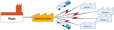
We can define the Just-in-time logistics structure by a production unit and a distribution network (size, number and location) of the different retailers specified by a single product, as show in Figure 2.
Figure 2. Structure studies
Assumptions
The main assumptions are as follows:
Objective
Minimizing the total cost of structure logistic.
We will introduce the mathematical formulation of Mixed Integer Linear Programming (MILP) in this next part.
2.2 Problem formulation
Objectif function
MinZ=T∑t=1(Production cos+Distribution Center cost)+T∑t=1NR∑i=1(Retailers cost) (1a)
\begin{aligned} & \operatorname{Min} Z=\sum_{t=1}^T\left(f p_i \boldsymbol{y}_t+p_i \boldsymbol{x}_{\boldsymbol{t}}\right)+\left(f d_t \boldsymbol{y} \boldsymbol{d}_{\boldsymbol{t}}+s d_t \boldsymbol{I} \boldsymbol{d}_{\boldsymbol{t}}\right)+\sum_{t=1}^T \sum_{i=1}^{N R}\left(f r_{i t} \boldsymbol{y} r_{i t}+s r_{i t} I \boldsymbol{r}_{i t}\right) \\ & \operatorname{Min} Z 2=\sum_{t=1}^T\left(f p_i \boldsymbol{y}_{\boldsymbol{t}}+p_i \boldsymbol{x}_{\boldsymbol{t}}\right)+\left(f d_t \boldsymbol{y} \boldsymbol{d}_{\boldsymbol{t}}+s d_t \boldsymbol{I} \boldsymbol{d}_{\boldsymbol{t}}\right)+\sum_{t=1}^T \sum_{i=1}^{N R}\left(f r_{i t} \boldsymbol{y} r_{i t}+s r_{i t} \boldsymbol{I} \boldsymbol{r}_{i t}\right)+\sum_{t=1}^T \sum_{i=1}^{N R}\left(u t_{i t} \boldsymbol{q} \boldsymbol{l}_{i t}\right)(1') \\ & \operatorname{Min} Z=\sum_{t=1}^T\left(f p_i \boldsymbol{y}_{\boldsymbol{t}}+p_i \boldsymbol{x}_{\boldsymbol{t}}\right)+\left(f d_t \boldsymbol{y} \boldsymbol{d}_{\boldsymbol{t}}+s d_t \boldsymbol{I} \boldsymbol{d}_{\boldsymbol{t}}\right)+\sum_{t=1}^T \sum_{i=1}^{N R}\left(f r_{i t} \boldsymbol{y} \boldsymbol{r}_{i t}+s r_{i t} \boldsymbol{I} \boldsymbol{r}_{i t}\right)+\sum_{t=1}^T \sum_{i=1}^{N R}\left(u t_{i t} \boldsymbol{q} \boldsymbol{l}_{\boldsymbol{i t}}\right) \\ & \end{aligned} (1b)
Subject to
The production capacity constraint
{{x}_{t}}\le {{y}_{t}}ca{{p}_{t}} (2)
The inventory level of DC and retailers’ constraints
I d_t=I d_{t-1}+x_t-\sum_{i=1}^{N R} d_{i t} (3)
I{{r}_{it}}=I{{r}_{it-1}}+q{{l}_{it}}-{{d}_{it}} (4)
The PM emission constraint
\sum_{k=1}^t\left(p e_k^m-P E_k^m\right) x_k \leq 0 (5)
h_{t}^{m}=h_{t-1}^{m}-\left( pe_{k}^{m}-PE_{k}^{m} \right){{x}_{t}} (6)
{{h}_{t}}\ge 0~;~{{h}_{0}}=0 (7)
The domain of definition of decision variables
x_t,\ I d_t,\ I r_{i t} \geq 0;\ intergers \forall\ \mathrm{i},\ \mathrm{t},\ \mathrm{k} (8)
The definition of decision variables
y_t=\left\{\begin{array}{c}0 \text { if } x_t=0 \\ 1 \text { Otherwise }\end{array}\right. (9)
y d_t=\left\{\begin{array}{c}0 \text { if } I d_t=0 \\ 1 \text { Otherwise }\end{array}\right. (10)
y r_{i t}=\left\{\begin{array}{l}0 \text { if } I d_t=0 \\ 1 \text { Otherwise }\end{array}\right. (11)
Table 2 presents the measurements of these particles over a 2018-2019 horizon in this company.
Table 2. Presentation of dust measurements in 2018-2019 at the cement industry in SKIKDA, Algeria
|
|
2018 |
2019 |
||
|
Location |
Production Tons |
Particle Matter (Mg/Nm³) |
Production Tons |
Particle Matter (Mg/Nm³) |
|
GP120 Filter |
1008783.84 |
25.67 |
1086120.3 |
30.92 |
|
Handle filter outlet L01 |
0.81 |
6.34 |
||
|
Handle filter outlet L02 |
0.78 |
3.72 |
||
|
L01 Chiller Bag Filter Outlet |
0.68 |
2.16 |
||
|
L02 Chiller Bag Filter Outlet |
1.21 |
1.65 |
||
Table 3 explains the principle of inventory emission variable.
Table 3. Example for cumulative emission
|
t |
x |
pe |
Emission |
PE |
pe-PE |
x(pe-PE) |
H |
|
1 |
100 |
10 |
1000 |
15 |
-5 |
-500 |
500 |
|
2 |
120 |
5 |
600 |
10 |
-5 |
-600 |
1100 |
|
3 |
50 |
15 |
750 |
17 |
-2 |
-100 |
1200 |
|
4 |
0 |
17 |
0 |
20 |
-3 |
0 |
1200 |
|
5 |
250 |
10 |
2500 |
15 |
-5 |
-1250 |
2450 |
|
6 |
25 |
9 |
225 |
10 |
-1 |
-25 |
2475 |
|
7 |
40 |
12 |
480 |
10 |
2 |
80 |
2395 |
|
8 |
90 |
8 |
720 |
4 |
4 |
360 |
2035 |
|
9 |
0 |
14 |
0 |
8 |
6 |
0 |
2035 |
|
10 |
200 |
5 |
1000 |
5 |
0 |
0 |
2035 |
In Table 3, example for cumulative emission {{\text{h}}_{\text{t}}} values increase until t=6, because \text{P}{{\text{E}}_{\text{t}}} is greater then \text{p}{{\text{e}}_{\text{t}}} (\text{P}{{\text{E}}_{\text{t}}}>\text{p}{{\text{e}}_{\text{t}}}); it means permission is sufficient for production. Till \text{t}=7 h decrease \text{P}{{\text{E}}_{\text{t}}} is less then \text{p}{{\text{e}}_{\text{t}}} (\text{P}{{\text{E}}_{\text{t}}}<\text{p}{{\text{e}}_{\text{t}}}), it means we need permissions from inventory emission to produce x quantity. This is what explain clearly Figure 3. In another manner:
For t=1 to T do
If \text{P}{{\text{E}}_{\text{t}}}\text{*}{{\text{x}}_{\text{t}}}>\text{p}{{\text{e}}_{\text{t}}}{{\text{x}}_{\text{t}}} then
Do not need {{\text{h}}_{\text{t}}}
Else
Need {{\text{h}}_{\text{t}}}
End.
Figure 3. Cumulative emission
Another scenario presents itself, when h takes negative values; that mean in this period plant cannot produce all quantity desired because it has not permission for particle emission. It has consumed all its reserve during the previous periods. Therefore, in this case plant must reduce production to get at least zero inventory of emission and satisfy environmental constraint.
After we have defined the mathematical model in MIPL with different constraints, we will go through proposing a way to solve this problem.
3.1 The basis of PSO
Particle swarm optimization (PSO) is developed by Kennedy and Eberhart, and it the main product is through consistency and competition by conveying specific information to guide the improvement process [36].
|
Algorithm General PSO |
|
Begin |
|
Initialize randomly swarm, velocity/*a set of particles |
|
Calculate Pbest, Gbest |
|
For i=1 to NI/*number of iterations |
|
Calculate new velocity |
|
Calculate new swarm |
|
Calculate Pbest and Gbest Seek fitness |
|
End for |
|
Write fitness/*the best value from all. |
|
End |
Now we adopt this algorithm to solve capacitated lot-sizing problem.
3.2 Structure of the binary PSO algorithm
Better efficiency of PSO -based search could be achieved by modifying the particle representation and its related operators to generate feasible solutions [37].
Sazvar et al. [14] proposed an integer presentation of the particle; each particle refers to the number of batch sizes ordered for each product for each period to solve a supply chain with perishable items. Boonmee and Sethanan [38] developed a new decoding representation where each particle in the swarm is separated into two parts, to solve multi-level capacitated lot-sizing and scheduling problems. The first part is the number of chicks purchased and delivered to the poultry industry in each period, and the second part is the allocation of chicks and pullets to farms.
However, Chen and Lin [39] developed a representation of complex particles encoding type is integers, while Izakian et al. [40] only encoded with binary values, which speeds up the algorithm and deals with large solution spaces.
We have designed an effective particle representation with an accelerated algorithm on the basis of the analysis of the approach adopted from the above literature. PSO simulates the movement of a group of volatile particles. It can search very large spaces of candidate solutions.
Now, we adopt this algorithm to solve capacitated lot-sizing problem.
3.2.1 Binary particle encoding
In this case, we use two particles:
(1) {{L}_{it}}: binary matrix L_{i t}=\left[\begin{array}{lllllll}1 & 0 & 0 & 1 & 0 & 1 & 0 \\ 1 & 1 & 0 & 0 & 0 & 1 & 0 \\ 1 & 0 & 0 & 0 & 1 & 1 & 1\end{array}\right]
(2) y_t=\left[\begin{array}{lllllll}1 & 0 & 0 & 1 & 0 & 0 & 1\end{array}\right]
3.2.2 Calculating fitness
To calculate z, we need all the values of decision variables {{x}_{t}},\text{ }\!\!~\!\!\text{ }I{{d}_{t}},\text{ }\!\!~\!\!\text{ }I{{r}_{it}},\text{ }\!\!~\!\!\text{ }y{{d}_{t}},y{{r}_{it}}, from particles one; such parameters are mentioned in Figure 4, which illustrates the way of calculation.
Figure 4. Way for calculation
|
Algorithm quantity delivered |
|
Begin |
|
ql=0 |
|
For i=1 to NR do |
|
For t=1 to T |
|
If L(i,t)=1 |
|
ql(i;t)=d(i;t) |
|
k=t |
|
Else |
|
While L(i,t)=0 |
|
ql(i;k)= ql(i;k)+d(i;t) |
|
t=t+1 |
|
End for |
|
Ir(I, t)=Ir(I,t-1)+ql(i,t)-d(i,t) |
|
If Ir(i, t)= 0 then |
|
yr(i, t)=0 Else |
|
yr(i, t)=1 |
|
End if |
The next step is to find the produced quantity. We should use the delivered quantity instead of the demand written in the produced quantity algorithm.
|
Algorithm quantity produced |
|
Begin |
|
x=0; h=0 |
|
For t=1 to T do |
|
If y(t)=1 |
|
x(t)=sum ql(i; t) if \mathbf{PE}\left( \mathbf{t} \right)>\mathbf{pe}\left( \mathbf{t} \right) then h=h+(PE(t)-pe(t)); end |
|
k=t |
|
Else |
|
While y(t)=0 and x(k)\le cap(t) and \mathbf{p}\le \mathbf{h} |
|
x(k)=x(k)+sum ql(i,t) h=h+(PE(t)-pe(t)); |
|
t=t+1 |
|
End while |
|
If (x(k)>cap(t) or pe(t)>PE(t) then/*test constraint capacity and CAP emission |
|
x(k)=x(k)-sum ql(i, t) |
|
Y(t)=1 |
|
End if |
|
t=t-1 |
|
Id(t)=Id(t-1)+x(t)-sum ql(i, t) |
|
End for |
|
If Id(t)=0 then |
|
yd(t)=0 Else |
|
yd(t)=1 |
|
End if |
|
End |
Everything is ready to calculate fitness. The next step is to use PSO to solve the capacitated lot-sizing problems.
3.2.3 Binary PSO algorithm
(1) Generate randomly X such as
X\left( i,t,p \right)=\left[ \begin{matrix} y \\ L \\\end{matrix} \right]=\left[ \begin{matrix} \left[ \begin{matrix} 1 & 0 & \begin{matrix} 0 & 1 & \begin{matrix} 0 & 0 & 1 \\\end{matrix} \\\end{matrix} \\\end{matrix} \right] \\ \left[ \begin{matrix} \begin{matrix} 1 & 0 & 0 \\ 1 & 1 & 0 \\ 1 & 0 & 0 \\\end{matrix} & \begin{matrix} 1 & 0 & 1 \\ 0 & 0 & 1 \\ 0 & 1 & 1 \\\end{matrix} & \begin{matrix} 0 \\ 0 \\ 1 \\\end{matrix} \\\end{matrix} \right] \\\end{matrix} \right]
where, i=1, i=1, t=7, p=1
(2) Generate randomly~V in \left[ -v;\text{ }\!\!~\!\!\text{ }+v \right] when Dim [X]=Dim [V]
(3) Calculate fitness gbest and pbest as shown in Table 4.
Table 4. Fitness values
|
P |
Iter1 |
Iter2 |
Iter3 |
Iter4 |
|
1 |
25 |
20 |
18 |
16 |
|
2 |
40 |
35 |
25 |
15 |
|
3 |
20 |
19 |
30 |
25 |
|
4 |
60 |
45 |
20 |
22 |
(4) Next iterations to calculate the new velocity V for~V_{\left( i,t,p \right)}^{iter+1}
Using the following equation:
\begin{array}{r}V_{(i, t, p)}^{iter+1}=\omega V_{(i, t, p)}^{iter}+C 1 r 1\left(pbest^{iter}-X_{(i, t, p)}^{i t e r}\right) +C 2 r 2\left(gbest^{iter}-X_{(i, t, p)}^{i t e r}\right)\end{array} (12)
(5) Calculate new X, X_{(i, t, p)}^{\text {iter }+1}=\left\{\begin{array}{c}1 \text { if } \operatorname{Sig}\left(V_{(i, t, p)}^{i t e r+1}>r\right) \\ 0 \text { otherwise }\end{array}\right.
Such as Sig=\frac{1}{1+e^{-V_{(i, t, p)}^{i t e r+1}}}
In Figure 5, the detailed procedure of the Binary Particle Swarm Optimization for the planning problem with OWMR.
Figure 5. Framework of the proposed BPSO
In order to investigate the performance of the proposed algorithm (BPSO), a concrete analysis of the proposed algorithm is made. The BPSO is coded on Lenovo PC with 8G RAM and 2GHz. The software is MATLAB 2013. I have run my proposed algorithm for ten times on the same instance with the same best values of the selected parameters as it is shown in Table 5 [41-43].
Table 5. The best parameters values for BPSO
|
Parameters |
Values |
Best Parameters |
|
\omega |
[1,10] |
1 |
|
C1 |
[1,4] |
3 |
|
C2 |
[1,4] |
3 |
|
P |
[50,200] |
100 |
|
V |
[10,90] |
50 |
The instance problems case for the planning problem with OWMR under environment (PM emission) constraint are presented as following (see Table 6):
Table 6. Instances variation for the proposed BPSO
|
T |
NR |
T |
NR |
T |
NR |
|
Small size |
Medium size |
Big size |
|||
|
3,6,9,12 |
[2,10] |
15,18,21,27 |
[5,25] |
40,50,60,70 |
[30,70] |
• Case 1: little size/30 instance problems/(T\in [3;12], NR\in [2; 10])
• Case 2: middle size/30 instance problems (T\in [15; 27], NR\in [5; 25])
• Case 3: great size/30 instance problems/(T\in [40; 70], NR\in [30; 70])
Table 7 displays the computational results of our proposed BPSO. In this table, the problem instances are listed in the first column, the second PM emissions and the third columns represent the number of period and retailers respectively, the fourth and five column that refer to our algorithms are still compared with CPLEX lower bound.
Table 7. Performance of BPSO
|
Little size |
Instances |
PM Emission |
T |
NR |
T*NR |
PSO |
CPLEX |
Err |
||||
|
PE |
Pe |
ZPSO |
Time(s) |
ZCPLEX |
Time (s) |
|||||||
|
1 |
1 |
U[3,6] |
U[2,5] |
3 |
2 |
6 |
1030 |
27.931 |
1030 |
0.614 |
0 |
|
|
2 |
2 |
U[3,6] |
U[2,5] |
3 |
4 |
12 |
574 |
61.1 |
575 |
1.343 |
0 |
|
|
3 |
3 |
U[3,6] |
U[2,5] |
6 |
2 |
12 |
1311 |
54.977 |
1295 |
1.208 |
0.01 |
|
|
4 |
4 |
U[3,6] |
U[2,5] |
3 |
6 |
18 |
2953 |
65.26 |
2954 |
1.434 |
0 |
|
|
5 |
5 |
U[3,6] |
U[2,5] |
6 |
3 |
18 |
587 |
60.45 |
589 |
1.302 |
0 |
|
|
6 |
6 |
U[3,6] |
U[2,5] |
9 |
2 |
18 |
3732 |
60.918 |
3589 |
1.339 |
0.04 |
|
|
7 |
7 |
U[3,6] |
U[2,5] |
3 |
8 |
24 |
3831 |
33.709 |
3831 |
0.741 |
0 |
|
|
8 |
8 |
U[3,6] |
U[2,5] |
6 |
4 |
24 |
3831 |
33.709 |
3794 |
0.741 |
0.01 |
|
|
9 |
9 |
U[3,6] |
U[2,5] |
12 |
2 |
24 |
4982 |
62.244 |
4152 |
1.368 |
0.2 |
|
|
10 |
10 |
U[3,6] |
U[2,5] |
3 |
9 |
27 |
5841 |
67.205 |
5841 |
1.469 |
0 |
|
|
11 |
11 |
U[3,6] |
U[2,5] |
9 |
3 |
27 |
9653 |
33.835 |
9553 |
0.819 |
0.01 |
|
|
12 |
12 |
U[3,6] |
U[2,5] |
3 |
10 |
30 |
7325 |
36.504 |
7261 |
0.802 |
0.01 |
|
|
13 |
13 |
U[3,6] |
U[2,5] |
6 |
5 |
30 |
8652 |
33.705 |
8635 |
0.823 |
0 |
|
|
14 |
14 |
U[3,6] |
U[2,5] |
6 |
6 |
36 |
5906 |
130.52 |
5791 |
2.869 |
0.02 |
|
|
15 |
15 |
U[3,6] |
U[2,5] |
9 |
4 |
36 |
5870 |
66.989 |
5755 |
1.472 |
0.02 |
|
|
16 |
16 |
U[3,6] |
U[2,5] |
9 |
5 |
45 |
9565 |
67.301 |
9326 |
1.467 |
0.02 |
|
|
17 |
17 |
U[3,6] |
U[2,5] |
6 |
8 |
48 |
7662 |
67.405 |
7439 |
1.482 |
0.03 |
|
|
18 |
18 |
U[3,6] |
U[2,5] |
12 |
4 |
48 |
9197 |
70.07 |
7075 |
1.54 |
0.3 |
|
|
19 |
19 |
U[3,6] |
U[2,5] |
6 |
9 |
54 |
9383 |
73.098 |
9122 |
1.6 |
0.03 |
|
|
20 |
20 |
U[3,6] |
U[2,5] |
9 |
6 |
54 |
17012 |
73.086 |
16421 |
1.606 |
0.04 |
|
|
21 |
21 |
U[3,6] |
U[2,5] |
6 |
10 |
60 |
14651 |
73.008 |
14406 |
1.605 |
0.02 |
|
|
22 |
22 |
U[3,6] |
U[2,5] |
12 |
5 |
60 |
14651 |
73.326 |
14406 |
1.626 |
0.02 |
|
|
23 |
23 |
U[3,6] |
U[2,5] |
9 |
8 |
72 |
11919 |
79.014 |
11572 |
1.737 |
0.03 |
|
|
25 |
25 |
U[3,6] |
U[2,5] |
12 |
6 |
72 |
11700 |
79.313 |
8299 |
1.743 |
0.41 |
|
|
26 |
26 |
U[3,6] |
U[2,5] |
15 |
5 |
75 |
5952 |
82.654 |
3608 |
1.816 |
0.65 |
|
|
27 |
27 |
U[3,6] |
U[2,5] |
9 |
9 |
81 |
9565 |
82.126 |
9326 |
1.923 |
0.02 |
|
|
28 |
28 |
U[3,6] |
U[2,5] |
9 |
10 |
90 |
21803 |
86.489 |
14536 |
1.901 |
0.5 |
|
|
29 |
29 |
U[3,6] |
U[2,5] |
12 |
8 |
96 |
16971 |
89.284 |
11624 |
1.962 |
0.4 |
|
|
30 |
30 |
U[3,6] |
U[2,5] |
12 |
9 |
108 |
15245 |
91.326 |
10136 |
1.852 |
0.501 |
|
|
Middle size |
31 |
31 |
U[3,4] |
U[2,3] |
18 |
5 |
90 |
6892 |
85,501 |
1887 |
33.879 |
2.652 |
|
32 |
32 |
U[3,4] |
U[2,3] |
21 |
5 |
105 |
11771 |
91.286 |
2243 |
35.875 |
2.006 |
|
|
33 |
33 |
U[3,4] |
U[2,3] |
12 |
10 |
120 |
15140 |
97.955 |
9961 |
33.321 |
2.153 |
|
|
34 |
34 |
U[3,4] |
U[2,3] |
27 |
5 |
135 |
9661 |
103.35 |
1281 |
60.732 |
2.271 |
|
|
35 |
35 |
U[3,4] |
U[2,3] |
15 |
10 |
150 |
16887 |
108.212 |
8529 |
60.378 |
2.378 |
|
|
36 |
36 |
U[3,4] |
U[2,3] |
18 |
10 |
180 |
20284 |
117.195 |
8992 |
65.576 |
2.576 |
|
|
37 |
37 |
U[3,4] |
U[2,3] |
21 |
10 |
210 |
36845 |
129.675 |
7066 |
71.089 |
2.85 |
|
|
38 |
38 |
U[3,4] |
U[2,3] |
15 |
15 |
225 |
40385 |
136.695 |
17949 |
70.004 |
3.004 |
|
|
39 |
39 |
U[3,4] |
U[2,3] |
18 |
13 |
234 |
30254 |
137.025 |
7542 |
70.52 |
3.011 |
|
|
40 |
40 |
U[3,4] |
U[2,3] |
18 |
15 |
270 |
73815 |
152.321 |
18641 |
73.348 |
3.348 |
|
|
41 |
41 |
U[3,4] |
U[2,3] |
27 |
10 |
270 |
30805 |
152.75 |
4247 |
73.023 |
3.357 |
|
|
43 |
43 |
U[3,4] |
U[2,3] |
21 |
13 |
273 |
73262 |
152.98 |
15478 |
73.828 |
3.735 |
|
|
44 |
44 |
U[3,4] |
U[2,3] |
15 |
19 |
285 |
33585 |
165.25 |
8754 |
74.110 |
2.83 |
|
|
45 |
45 |
U[3,4] |
U[2,3] |
15 |
20 |
300 |
76534 |
165.386 |
33955 |
74.080 |
3.635 |
|
|
46 |
46 |
U[3,4] |
U[2,3] |
21 |
15 |
315 |
40363 |
160.417 |
6397 |
73.584 |
3.745 |
|
|
47 |
47 |
U[3,4] |
U[2,3] |
18 |
19 |
342 |
76982 |
171.123 |
11548 |
70.365 |
5.66 |
|
|
48 |
48 |
U[3,4] |
U[2,3] |
15 |
23 |
345 |
54576 |
170.502 |
11587 |
73.58 |
3.710 |
|
|
49 |
49 |
U[3,4] |
U[2,3] |
18 |
20 |
360 |
50575 |
189.371 |
15120 |
44.623 |
4.162 |
|
|
50 |
50 |
U[3,4] |
U[2,3] |
15 |
25 |
375 |
30120 |
196.586 |
8991 |
44.320 |
4.32 |
|
|
51 |
51 |
U[3,4] |
U[2,3] |
21 |
19 |
399 |
77895 |
200.93 |
13254 |
44.523 |
4.887 |
|
|
52 |
52 |
U[3,4] |
U[2,3] |
27 |
15 |
405 |
87628 |
201.76 |
10622 |
44.623 |
4.434 |
|
|
53 |
53 |
U[3,4] |
U[2,3] |
18 |
23 |
414 |
82585 |
205.36 |
15236 |
49.326 |
4.423 |
|
|
55 |
55 |
U[3,4] |
U[2,3] |
21 |
20 |
420 |
38178 |
213.98 |
5796 |
50.356 |
4.703 |
|
|
56 |
56 |
U[3,4] |
U[2,3] |
18 |
25 |
450 |
56901 |
225.81 |
13376 |
52.963 |
3.25 |
|
|
57 |
57 |
U[3,4] |
U[2,3] |
21 |
23 |
483 |
79852 |
223.52 |
13845 |
52.627 |
4.985 |
|
|
58 |
58 |
U[3,4] |
U[2,3] |
27 |
19 |
513 |
88956 |
225.66 |
15852 |
52.071 |
4.611 |
|
|
59 |
59 |
U[3,4] |
U[2,3] |
21 |
25 |
525 |
46904 |
227.27 |
9003 |
52.962 |
5.654 |
|
|
60 |
60 |
U[3,4] |
U[2,3] |
27 |
20 |
540 |
43615 |
256.62 |
4714 |
52.987 |
5.64 |
|
|
Great size |
61 |
61 |
U[2,4] |
U[1,3] |
40 |
30 |
1200 |
180659 |
538.2 |
18530 |
448.5 |
8.75 |
|
62 |
62 |
U[2,4] |
U[1,3] |
40 |
35 |
1400 |
338803 |
528.19 |
31459 |
440.158 |
9.77 |
|
|
63 |
63 |
U[2,4] |
U[1,3] |
50 |
30 |
1500 |
435249 |
661.31 |
41217 |
551.092 |
9.56 |
|
|
64 |
64 |
U[2,4] |
U[1,3] |
40 |
40 |
1600 |
227569 |
733.98 |
23015 |
611.65 |
8.89 |
|
|
65 |
65 |
U[2,4] |
U[1,3] |
50 |
35 |
1750 |
515273 |
777.53 |
51766 |
647.942 |
8.95 |
|
|
66 |
66 |
U[2,4] |
U[1,3] |
40 |
45 |
1800 |
178438 |
897.52 |
17402 |
747.933 |
9.25 |
|
|
67 |
67 |
U[2,4] |
U[1,3] |
60 |
30 |
1800 |
334717 |
789.1 |
28152 |
970.593 |
10.89 |
|
|
68 |
68 |
U[2,4] |
U[1,3] |
40 |
50 |
2000 |
186797 |
1006.33 |
22626 |
838.608 |
7.26 |
|
|
69 |
69 |
U[2,4] |
U[1,3] |
50 |
40 |
2000 |
548875 |
950.56 |
55125 |
792.133 |
8.96 |
|
|
70 |
70 |
U[2,4] |
U[1,3] |
40 |
52 |
2080 |
183852 |
973.83 |
19856 |
797.362 |
8.259 |
|
|
71 |
71 |
U[2,4] |
U[1,3] |
60 |
35 |
2100 |
305751 |
953.94 |
29830 |
1173.346 |
9.25 |
|
|
72 |
72 |
U[2,4] |
U[1,3] |
70 |
30 |
2100 |
379088 |
901.94 |
30231 |
2899.737 |
11.54 |
|
|
73 |
73 |
U[2,4] |
U[1,3] |
40 |
55 |
2200 |
182973 |
1109.73 |
17895 |
983.408 |
9.224 |
|
|
75 |
75 |
U[2,4] |
U[1,3] |
50 |
45 |
2250 |
664356 |
1109.81 |
57371 |
924.842 |
10.58 |
|
|
76 |
76 |
U[2,4] |
U[1,3] |
60 |
40 |
2400 |
365551 |
1119.3 |
36464 |
1376.739 |
9.03 |
|
|
77 |
77 |
U[2,4] |
U[1,3] |
70 |
35 |
2450 |
703450 |
1115.66 |
60176 |
3586.847 |
10.69 |
|
|
78 |
78 |
U[2,4] |
U[1,3] |
50 |
50 |
2500 |
776186 |
1300 |
61897 |
1599 |
11.54 |
|
|
79 |
79 |
U[2,4] |
U[1,3] |
40 |
65 |
2600 |
285658 |
1300.86 |
22025 |
1602.258 |
11.656 |
|
|
80 |
80 |
U[2,4] |
U[1,3] |
60 |
45 |
2700 |
399334 |
1301.56 |
36254 |
1600.919 |
10.02 |
|
|
81 |
81 |
U[2,4] |
U[1,3] |
50 |
55 |
2750 |
778985 |
1112.63 |
66584 |
964.057 |
10.699 |
|
|
82 |
82 |
U[2,4] |
U[1,3] |
70 |
40 |
2800 |
271554 |
1560 |
N/A |
N/A |
N/A |
|
|
83 |
83 |
U[2,4] |
U[1,3] |
60 |
50 |
3000 |
446246 |
3258.97 |
N/A |
N/A |
N/A |
|
|
84 |
84 |
U[2,4] |
U[1,3] |
50 |
65 |
3250 |
487589 |
1658.25 |
N/A |
N/A |
N/A |
|
|
85 |
85 |
U[2,4] |
U[1,3] |
60 |
55 |
3300 |
332557 |
4165.35 |
N/A |
N/A |
N/A |
|
|
86 |
86 |
U[2,4] |
U[1,3] |
70 |
55 |
3850 |
798258 |
1325.36 |
N/A |
N/A |
N/A |
|
|
87 |
87 |
U[2,4] |
U[1,3] |
60 |
65 |
3900 |
273854 |
2265.23 |
N/A |
N/A |
N/A |
|
|
88 |
88 |
U[2,4] |
U[1,3] |
70 |
60 |
4200 |
458272 |
2210.02 |
N/A |
N/A |
N/A |
|
|
89 |
89 |
U[2,4] |
U[1,3] |
70 |
65 |
4550 |
985025 |
3873.58 |
N/A |
N/A |
N/A |
|
|
90 |
90 |
U[2,4] |
U[1,3] |
70 |
70 |
4900 |
575092 |
4160 |
N/A |
N/A |
N/A |
|
For each instance, results are summarized in Table 7, in which we compare our proposed BPSO algorithms and CPLEX in terms of total cost {{Z}_{BPSO}} time and running Time(s).
• Little size
From Table 7 in the little size, the difference between {{Z}_{BPSO}}\text{ }\!\!~\!\!\text{ and }\!\!~\!\!\text{ }{{Z}_{CPLEX}} is \text{Err}\in [0; 0.65] s is small, when BPSO speed reaches 0.65s, it gives us solution optimal. We have also noticed a proportionality between the running time and (T, NR).
• Middle size
From Table 7 in the Middle size, the difference between {{Z}_{BPSO}}\text{ }\!\!~\!\!\text{ and }\!\!~\!\!\text{ }{{Z}_{CPLEX}} is \text{Err}\in [0.98; 3.29] s for an increased instance (T, NR), and the Err increases too. We have also noticed a proportionality between the running time and (T, NR).
• Great size
From Table 7 in Great size, the difference between {{Z}_{BPSO}}\text{ }\!\!~\!\!\text{ and }\!\!~\!\!\text{ }{{Z}_{CPLEX}} is \text{Err}\in[7.26; 11.65] s for an increased instance (T, NR) and the Err increases more as well.
Err=\frac{{{Z}_{PSO}}-{{Z}_{CPLEX}}}{{{Z}_{CPLEX}}}
The running time BPSO is better than CPLEX.
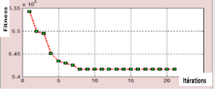
Figure 6 depicts the convergence behavior of BPSO for the (T=50 and NR=40) instance. This figure shows the improvement of average solution quality of this instance over the number of Iterations.
Figure 6. Decrease of cost function
Figure 7 illustrates the running time (s) (BPSO, CPLEX). The running time is exponential linear.
Figure 7. The running time (BPSO-CPLEX)
Most of the research’s scholars are interested in integrating carbon emission constraint within the lot-sizing problem. In this article, we have focused on integrating hard particles different in their nature. These emissions contribute riskily to increasing air pollution, which negatively affects the environment, especially by major industrial companies, in general, and companies of construction materials and cement, in particular. In this article, we have solved a lot-sizing problem. The description model of this later is production unit and a distribution network (size, number and location) in different retailers in time under cumulative particulate matters emission constraint.
A mixed-integer programming model has been constructed the problem is NP-hard. We have developed a binary particle swarm optimization one for solving it. The BPSO approach that was proposed is powerful and delivers high-quality solutions within a short running time.
Based on the discussions and analysis of this study trend of Binary swarm intelligence optimization for solving the green lot-sizing problem,
Through this study, we have developed a specialized software that is also a decision support system Creates a decision support system to help business managers make decisions in time and space, quantity to trigger production and distribute in a sustainable environment while satisfying the customer at the lowest total cost and on the other hand respecting cumulative emissions.
We give some perspectives from the problems aspects, approaches and constraints for future works.
• The real-world constraints must be considered if we want to solve lot-sizing problem in the various industrial environments. Through considering the real-life constraints, we can put the planning results included within the theoretical research into a specific field or a specific transport and products storage as a helping tool for making decision.
• Minimizing energy consumption in transports and production are two new objectives to seek in integrating the problem of turning the vehicle and production scheduling problems with the green lot-sizing problem.
• Efficient hybrid swarm intelligence optimization with the local search is vital for solving the green lot-sizing problem.
• The models and planning strategies for multi-product and multi-objective optimization remain a challenging issue, which needs to be further studied for the lot-sizing problem.
• Comparing the results of the study with metaheuristic such as ant colonies
National Higher School of Technology and Engineering has generously supported the research. The author would like to express their sincere appreciation for all support provided. We would like to thank Pr. A. Driss and R. Zeggada for checking our English phrasing.
|
Indices |
|
|
T |
Number of periods |
|
NR |
Number of retailers |
|
t |
Index of periods, \text{t}=1, 2, ..., T |
|
i |
Index of retailers,\text{ }\!\!~\!\!\text{ i}=1, 2, ..., NR |
|
M |
Number of particulate matters |
|
m |
Index of particulate matters m=1, 2, …M |
|
Parameters |
|
|
dit |
Amount of demand of retailer i at the end period t |
|
pe_{k}^{m} |
PM emission quota per unitary product in |
|
PE_{k}^{m} |
Maximum unitary PM emission per period |
|
Production |
|
|
Capt |
Total production capacity of plant during period t |
|
pt |
Unitary cost of production |
|
fpt |
Setup cost of production |
|
Delivery |
|
|
utt |
delivery cost for unit of product |
|
Holding |
|
|
sdt |
Unitary holding cost for distribution center in period \text{i} |
|
fdt |
Setup cost for distribution center in period i |
|
srit |
Unitary holding cost for retailer \text{i} in period t |
|
frit |
Setup cost for retailer \text{i} in period t |
|
Variable decision |
|
|
xt |
Quantity produced in period t |
|
yt |
Binary variable there is or no production in period t |
|
idt |
Inventory level in distribution center at period t |
|
ydt |
Binary variable there is or no stock in DC in period t |
|
irit |
Inventory level for retailer i in period t |
|
yrit |
Binary variable there is or no stock in retailer i in period t |
|
qlrit |
Quantity delivered to retailer I at period t |
|
X |
Swarm of particles |
|
p |
Index of swarm |
|
P |
Maximum number of particles |
|
iter |
Index of iterations |
|
ω |
Inertia weight |
|
C1, C2 |
Positive acceleration which control the influence of gbest and pbest in search process |
|
r1, r2, r |
Random variable uniform distribution |
[1] Sarker, B.R. (2014). Consignment stocking policy models for supply chain systems: A critical review and comparative perspectives. International Journal of Production Economics, 155: 52-67. https://doi.org/10.1016/j.ijpe.2013.11.005
[2] Tempelmeier, H., Hilger, T. (2015). Linear programming models for a stochastic dynamic capacitated lot sizing problem. Computers & Operations Research, 59: 119-125.https://doi.org/10.1016/j.cor.2015.01.007
[3] Lee, A.H., Kang, H.Y., Lai, C.M., Hong, W.Y. (2013). An integrated model for lot sizing with supplier selection and quantity discounts. Applied Mathematical Modelling, 37(7): 4733-4746. https://doi.org/10.1016/j.apm.2012.09.056
[4] Rapine, C., Penz, B., Gicquel, C., Akbalik, A. (2018). Capacity acquisition for the single-item lot sizing problem under energy constraints. Omega, 81: 112-122. https://doi.org/10.1016/j.omega.2017.10.004
[5] Manikas, A., Godfrey, M. (2010). Inducing green behavior in a manufacturer. Global Journal of Business Research, 4(2): 27-38.
[6] El Saadany, A.M.A., Jaber, M.Y., Bonney, M. (2011). Environmental performance measures for supply chains. Management Research Review, 34(11): 1202-1221. https://doi.org/10.1108/01409171111178756
[7] Hua, G., Cheng, T.C.E., Wang, S. (2011). Managing carbon footprints in inventory management. International Journal of Production Economics, 132(2): 178-185. https://doi.org/10.1016/j.ijpe.2011.03.024
[8] Bouchery, Y., Ghaffari, A., Jemai, Z., Dallery, Y. (2012). Including sustainability criteria into inventory models. European Journal of Operational Research, 222(2): 229-240.https://doi.org/10.1016/j.ejor.2012.05.004
[9] Benjaafar, S., Li, Y., Daskin, M. (2012). Carbon footprint and the management of supply chains: Insights from simple models. IEEE Transactions on Automation Science and Engineering, 10(1): 99-116.https://doi.org/10.1109/TASE.2012.2203304
[10] Absi, N., Dauzère-Pérès, S., Kedad-Sidhoum, S., Penz, B., Rapine, C. (2013). Lot sizing with carbon emission constraints. European Journal of Operational Research, 227(1): 55-61. https://doi.org/10.1016/j.ejor.2012.11.044
[11] Dye, C.Y., Yang, C.T. (2015). Sustainable trade credit and replenishment decisions with credit-linked demand under carbon emission constraints. European Journal of Operational Research, 244(1): 187-200. https://doi.org/10.1016/j.ejor.2015.01.026
[12] Palak, G., Ekşioğlu, S.D., Geunes, J. (2014). Analyzing the impacts of carbon regulatory mechanisms on supplier and mode selection decisions: An application to a biofuel supply chain. International Journal of Production Economics, 154: 198-216. https://doi.org/10.1016/j.ijpe.2014.04.019
[13] Nouira, I., Hammami, R., Frein, Y., Temponi, C. (2016). Design of forward supply chains: Impact of a carbon emissions-sensitive demand. International Journal of Production Economics, 173: 80-98. https://doi.org/10.1016/j.ijpe.2015.11.002
[14] Sazvar, Z., Mirzapour Al-e-hashem, S.M.J., Govindan, K., Bahli, B. (2016). A novel mathematical model for a multi-period, multi-product optimal ordering problem considering expiry dates in a FEFO system. Transportation Research Part E: Logistics and Transportation Review, 93: 232-261. https://doi.org/10.1016/j.tre.2016.04.011
[15] Jaber, M.Y., Glock, C.H., El Saadany, A.M. (2013). Supply chain coordination with emissions reduction incentives. International Journal of Production Research, 51(1): 69-82. https://doi.org/10.1080/00207543.2011.651656
[16] Florian, M., Klein, M. (1971). Deterministic production planning with concave costs and capacity constraints. Management Science, 18(1): 12-20. https://doi.org/10.1287/mnsc.18.1.12
[17] Bonney, M., Jaber, M.Y. (2011). Environmentally responsible inventory models: non classical models for a non-classical era. International Journal of Production Economics, 133(1): 43-53. https://doi.org/10.1016/j.ijpe.2009.10.033
[18] Mirabelli, G., Solina, V. (2022). Optimization strategies for the integrated management of perishable supply chains: A literature review. Journal of Industrial Engineering and Management, 15(1): 58-91. https://doi.org/10.3926/jiem.3603
[19] Song, J.P., Leng, M.M. (2012). Analysis of the single-period problem under carbon emissions policies. In: Choi, TM. (eds) Handbook of Newsvendor Problems. International Series in Operations Research & Management Science, vol. 176. Springer, New York, NY. https://doi.org/10.1007/978-1-4614-3600-3_13
[20] Chen, X., Benjaafar, S., Elomri, A. (2013). The carbon-constrained EOQ. Operations Research Letters, 41(2): 172-179. https://doi.org/10.1016/j.orl.2012.12.003
[21] Zhang, G.Q., Ma, L.P. (2009). Optimal acquisition policy with quantity discounts and uncertain demands. International Journal of Production Research, 47(9): 2409-2425. https://doi.org/10.1080/00207540701678944
[22] Zhang, M.J., Kucukyavuz, S., Yaman, H. (2012). A polyhedral study of multi-echelon lot sizing with intermediate demands. Operations Research, 60(4): 918-935. https://doi.org/10.1287/opre.1120.1058
[23] Zhang, Z.H., Jiang, H., Pan, X.Z. (2012). A Lagrangian relaxation based approach for the capacitated lot sizing problem in closed-loop supply chain. International Journal of Production Economics, 140(1): 249-255. https://doi.org/10.1016/j.ijpe.2012.01.018
[24] Zhang, B., Xu, L., (2013). Multi-item production planning with carbon cap and trade mechanism. International Journal of Production Economics, 144(1): 118-127. https://doi.org/10.1016/j.ijpe.2013.01.024
[25] Rosic, H., Jammernegg, W. (2013). The economic and environmental performance of dual sourcing: A newsvendor approach, International Journal of Production Economics, 143(1): 109-119. https://doi.org/10.1016/j.ijpe.2012.12.007
[26] Konur, D., Schaefer, B. (2014). Integrated inventory control and transportation decisions under carbon emissions regulations: LTL vs. TL carriers. Transportation Research Part E: Logistics and Transportation Review, 68: 14-38. https://doi.org/10.1016/j.tre.2014.04.012
[27] Ghosh, A., Jha, J.K., Sarmah, S.P. (2017). Optimal LoT-sizing under strict carbon cap policy considering stochastic demand. Applied Mathematical Modelling, 44: 688-704. https://doi.org/10.1016/j.apm.2017.02.037
[28] Fahimnia, B., Sarkis, J., Choudhary, A., Eshragh, A. (2015). Tactical supply chain planning under a carbon tax policy scheme: A case study. International Journal of Production Economics, 164: 206-215. https://doi.org/10.1016/j.ijpe.2014.12.015
[29] Hammami, R., Nouira, I., Frein, Y. (2015). Carbon emissions in a multi-echelon production-inventory model with lead time constraints. International Journal of Production Economics, 164: 292-307. https://doi.org/10.1016/j.ijpe.2014.12.017
[30] He, Y., Li, Y., Wu, T., Sutherland, J. (2015). An energy-responsive optimization method for machine tool selection and operation sequence in flexible machining job shops. Journal of Cleaner Production, 87(1): 245-254. https://doi.org/10.1016/j.jclepro.2014.10.006
[31] Martí, J.M.C., Tancrez, J.S., Seifert, R.W. (2015). Carbon footprint and responsiveness trade-offs in supply chain network design. International Journal of Production Economics, 166: 129-142. https://doi.org/10.1016/j.ijpe.2015.04.016
[32] Koca, E., Yaman, H., Aktürk., M.S. (2015). Stochastic lot sizing problem with controllable processing times. Omega, 53: 1-10. https://doi.org/10.1016/j.omega.2014.11.003
[33] Zhou., S.H., Zhou, Y.L., Zuo, X.R., Xiao, Y.Y., Cheng Y. (2018). Modeling and solving the constrained multi-items lot-sizing problem with time-varying setup cost. Chaos, Solitons and Fractals, 116: 202-207. https://doi.org/10.1016/j.chaos.2018.09.012
[34] Purohit, A.K., Shankar, R., Dey, K.P., Choudhary, A. (2016). Non-stationary stochastic inventory lot-sizing with emission and service level constraints in a carbon cap-and-trade system. Journal of Cleaner Production, 113: 654-661. https://doi.org/10.1016/j.jclepro.2015.11.004
[35] Claassen G.D.H., Kirst, P., Thai Thi Van, A., Snels, J.C.M.A., Guo, X., van Beek, P. (2024). Integrating time-temperature dependent deterioration in the economic order quantity model for perishable products in multi-echelon supply chains. Omega, 125: 103041. https://doi.org/10.1016/j.omega.2024.103041
[36] Kennedy, J., Eberhart, R. (1995). Particle swarm optimization. In Proceedings of ICNN'95-International Conference on Neural Networks, Perth, WA, Australia, pp. 1942-1948. https://doi.org/10.1109/ICNN.1995.488968
[37] Driss, I. (2021). Binary particle swarm optimization for one warehouse multi retailer problem with cumulative particulate matter constraint. In 2021 International Conference on Control, Automation and Diagnosis (ICCAD), Grenoble, France, pp. 1-6. https://doi.org/10.1109/ICCAD52417.2021.9638769
[38] Boonmee, A., Sethanan, K. (2016). A GLNPSO for multi-level capacitated lot-sizing and scheduling problem in the poultry industry. European Journal of Operational Research, 250(2): 652-665. https://doi.org/10.1016/j.ejor.2015.09.020
[39] Chen, Y.Y., Lin, J.T. (2009). A modified particle swarm optimization for production planning problems in the TFT Array process. Expert Systems with Applications, 36(10): 12264-12271. https://doi.org/10.1016/j.eswa.2009.04.072
[40] Izakian, H., Ladani, B.T., Abraham, A., Snasel, V. (2010). A discrete particle swarm optimization approach for grid job scheduling. International Journal of Innovative Computing, Information and Control, 6(9): 1-15.
[41] Han, Y., Tang, J., Kaku, I., Mu, L. (2009). Solving uncapacitated multilevel lot-sizing problems using a particle swarm optimization with flexible inertial weight. Computers & Mathematics with Applications, 57(11-12): 1748-1755. https://doi.org/10.1016/j.camwa.2008.10.024
[42] Pant, M., Thangaraj, R., Abraham, A. (2009). Particle swarm optimization: Performance tuning and empirical analysis. In Foundations of Computational Intelligence. Berlin, Heidelberg: Springer, pp. 101-128. https://doi.org/10.1007/978-3-642-01085-9_5
[43] Parapar, J., Vidal, M.M., Santos, J. (2012). Finding the best parameter setting: Particle swarm optimisation. In 2nd Spanish Conference on Information Retrieval, pp. 49-60.