May H. Abood*![]() | Hikmat N. Abdullah
| Hikmat N. Abdullah![]()
© 2024 The authors. This article is published by IIETA and is licensed under the CC BY 4.0 license (http://creativecommons.org/licenses/by/4.0/).
OPEN ACCESS
The spectrum sensing function plays a significant role in the performance of cognitive radio (CR). Spectrum sensing specifies if free channels exist and identifies free channels for secondary users, actively helping in the improvement of spectrum usage and recognizing available channels in CR systems. Cyclostationary feature detection (CFD) is a spectrum sensing method that detects signals depending on different characteristics such as carrier frequency, modulation types, cyclic frequency, and symbol rates with an extremely low signal-to-noise ratio. At low SNR, CFD achieves a detection process with a high computation complexity. This paper designs Enhanced Cyclostationary Detector complexity with improved detection speed performances. For the sake of minimizing system complexity, utilizing the advantages of the Haar wavelet transform and signed correlator method for estimating the cyclic spectra of a detected signal. The proposed method performance was evaluated over Rayleigh flat fading and AWGN channel that had low SNR values. The acquired simulation results indicated the efficiency of the proposed method in terms of reduction 70% in complexity, 60% in time, and 7% in memory storage, with improved detection performance that is about 8% compared to conventional method at low SNR values reach to -30dB.
spectrum sensing, cyclostationary feature detection, Haar wavelet transform, signed correlator, computational complexity, Rayleigh flat fading, AWGN channel, low SNR
Wireless device distribution and the requirement for faster data rate transmission have increased in recent years. Radio spectrum shortage has resulted from a crowded environment and spectrum congestion. As a result, new solutions to utilize unused spectrum bands and boost spectrum usage in dynamically changing contexts are required [1]. Cognitive radio approaches have recently been investigated to meet the needs of expanding wireless applications on a restricted frequency resource. Spectrum sensing techniques play a key role in cognitive radio networks [2]. Its key objective is to detect spectrum holes so Cognitive User is able to utilize it and monitor the signal activity of the Authorized User to make sure that when the authorized user utilizes the spectrum again, the cognitive user can immediately leave the relevant frequency spectrum. The previous fixed spectrum sensing approaches have been unable to react to dynamic modifying in spectrum requirements, resulting in issues such as spectrum passiveness and unbalanced use, complicating the supply-demand imbalance for spectrum resources. The SU's receiver detection model employs a traditional technique commonly referred to as binary hypothesis testing, in which H0 represents the PU absence and H1 represents the PU presence. Suppose that a CR user receives a signal with a hypothesis that is [1]:
$y(t)= \begin{cases}x(t)+w(t) & \text { for } H_1 \\ w(t) & \text { for } H_0\end{cases}$ (1)
where, y(t) is the received signal, x(t) is the PU's transmission signal, and w(t) is additive white Gaussian noise (AWGN). To distinguish between the hypotheses, a hypothesis test is used with a specific threshold derived from the likelihood errors on the SU receiver. In the hypothesis tests that employ the model given in Eq. (1), there are two types of errors. The first error is false alarm probability (Pf) which happens when the SU's receiver receives a PU signal while PU not exist. In spectrum sensing, the false alarm probability is an essential system parameter to determine the threshold in the hypothesis test. The other is the probability of missed detection (Pm) that happens when the SU's receiver sees no PU signal when the PU is present and it is equivalent to:
$P_m=1-P_d$ (2)
where, Pd is the probability of detection. The efficiency of the CR system is defined by the false alarm probability Pf and the detection probability Pd [1, 2]. Pd and Pf indicated as the following:
$P_f=\mathrm{P}\left(\gamma>\lambda / H_0\right)=e^{-\frac{(2 N+1) \lambda^2}{2 \delta^4}}$ (3)
$P_d=\mathrm{P}\left(\gamma>\lambda / H_1\right)=Q_1\left(\frac{\sqrt{2 \gamma}}{\delta}, \frac{\lambda}{\delta_B}\right)$ (4)
where, N is the number of samples, λ is the threshold and δ is the variance of the input signal:
$\lambda=\sqrt{\left(\left(-\log P_{f a}\right) * 2 * \delta_B^2\right)}$ (5)
where, Q1 () is the Q function, γ is the SNR and the value of δB can be calculated from the equation:
$\delta_B^2=\frac{(2 \gamma+1) \delta^4}{2 N+1}$ (6)
Cyclostationarity is found in a lot of modulated signals presented in communications and telemetry systems. The signal is characterized as a cyclostationary signal if its statistical properties exhibit periodicity. The statistical properties of a cyclostationary system vary over time regularly, and it indicates various signal features such as rate, frequency, anti-noise ability, and modulation type [3]. Cyclostationary methods, its second-order statistical parameters, can show less computations in time and memory in terms of simulation and experimentation, so they are studied by many researchers.
Zhang et al. [4] offered three low-complexity detection techniques that can reduce computing complexity. The algorithm analysis and practical findings reveal that the suggested techniques outperform other techniques involving BER performance and computational cost.
Hu et al. [5] presented FACA technique of acquiring the cycle frequencies of a cyclostationary signal efficiently through increasing FFT window.
Souza et al. [6] demonstrated a unique spectral sensing approach for detecting signals with nonlinear phase fluctuation over time. It relies on the angle-time cyclostationarity theorem, which employs transformations to the detected signal to limit the impacts of nonlinear phase variation. The acquired simulation results indicated enhanced outcomes as a result of the primary user detection rate heightened by approximately 8 dB.
Kadjo et al. [7] presented a blind detection method depending on the cyclostationary properties of received signals is developed to circumvent the limitations of spectrum detectors. The processing cost is reduced by using the FFT accumulation technique for estimating the cyclic spectrum of the received signal. The simulation results demonstrated that the detector can detect the existence of a communication signal with a very low SNR.
Mathew and Samuel [8] presented a unique low-complexity technique for extracting cyclic features of wideband signals in sub-Nyquist samples. Because of the sparse spectrum's use in wideband, sub-Nyquist sampling and cyclostationary feature detection are used at baseband for identifying the modulation technique with low computational complexity.
Abdullah et al. [9] presented a hybrid low-cost spectrum sensing approach with improved detection efficiency using energy and cyclostationary detectors. The approach is built in a way that the energy detector is considered at high SNR values to conduct the detection and cyclostationary detector at low SNR a with lower complexity is considered for aiding in accurate detection. The complexity is reduced by limiting the amount of sensing samples utilized in the time domain autocorrelation process and by employing the Sliding Discrete Fourier Transform (SDFT) rather than FFT.
In this study, a low-complexity cyclostationary detector is proposed. It uses low complexity frequency transform, correlator, and threshold setting algorithms while ensuring the same detection performance in the AWGN channel. The of the paper is organized as follows: in Section 2, conventional cyclostationary detector is described. Section 3, presents the proposed cyclostationary method. Section 4 illustrates the obtained simulation results with their evaluation, while Section 5 demonstrates the conclusions drawn throughout the research paper.
Several sensing methods have been proposed to detect the primary user presence. Examples of these techniques include energy detection, cyclostationary detection, and matched filter detection. Energy detection is relatively simple to implement and computationally efficient but is sensitive to noise as it does not distinguish between signal from noise. Matched filter-based detection requires some prior knowledge about the primary user signal as it compares the received to the reference waveform which may not always be available or accurate in practical scenarios as this information about the signal is often unavailable [10]. Cyclostationary feature detection (CFD) utilize of inherent periodicity in modulated signals, generally achieved through the coupling with sinusoidal carriers. By effectively detect and analyze this periodicity, the cognitive system can detect this the presence of the primary user in the signal. CFD can differentiate between noise signals and modulated signals using signal cyclic features. For lower SNRs, cyclostationary feature detection (CFD) detection performance is better but has higher computational complexity and detection time than matched filter and energy detector.
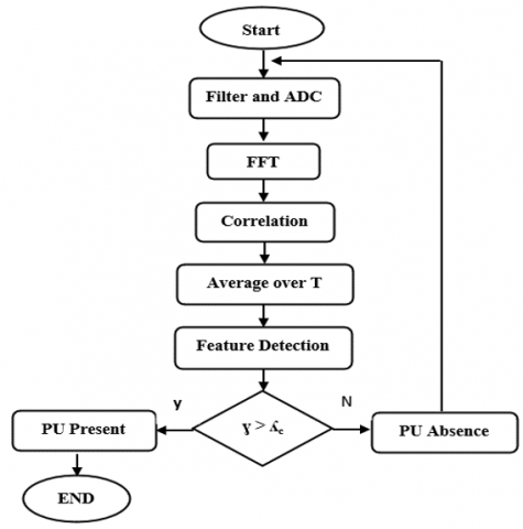
Figure 1. Cyclostationary feature detection
The cyclostationary feature detection approach is associated with detecting the inherent cyclostationary characteristics of a modulated signal using the knowledge that signals are typically combined with sine wave carriers, repeated spreading, pulse trains, or cyclic prefixes, resulting in periodicity. Statistics such as mean autocorrelation also demonstrate periodicity in a broad sense. Because this periodicity feature is employed to determine the presence of primary users, this approach performs satisfactorily in low SNR situations. Because noise is unpredictable and lacks periodicity, the noise-rejecting capability is quite strong in the scenario of cyclostationary feature detection [11]. As stationary signals are often examined using the autocorrelation function and power spectral density, cyclostationary signals are studied using generalizing of these functions known as the Cyclic Autocorrelation Function (CAF) and the Spectral-Correlation Density Function (SCD). Figure 1 shows the structures of the conventional cyclostationary feature detectors.
After signal is received from bandpass filter, the signal is sampled, then FFT of the sampled signal is computed and correlated with its conjugate in correlation stage then average data over period of T to reduce the effect of noise and used in feature detection stage where signal feature is detected to decision the presence or absence of PU.
A time-series $R_x^\alpha(\tau)$ is said to exhibit as the main parameter of second-order cyclostationarity (SOCS) in continuous time for some nonzero frequency α, called the cyclic frequency, is called Cyclic Autocorrelation Function (CAF) [11]:
$R_x^\alpha(\tau) \left\lvert\, \triangleq\left\langle x\left(t+\frac{\tau}{2}\right) x^*\left(t-\frac{\tau}{2}\right) e^{-i 2 \pi \alpha t}\right\rangle_0\right.$ (7)
CAF is representing the amount of correlation between different frequency shifted version of a signal. The signal is called cyclostationary if CAF is not zero for nonzero cyclic frequency α. If x(t) demonstrates SOCS, the second-order temporal instant for x(t) is given by:
$R_x(t, \tau) \triangleq\left\langle x\left(t+\frac{\tau}{2}\right) x^*\left(t-\frac{\tau}{2}\right)\right\rangle$ (8)
For each $\tau$, it is a periodic function of t. The moment function and the cyclic autocorrelation function are connected by Eqs. (6)-(7).
$R_x(t, \tau)=\sum_\alpha R_x^\alpha(\tau) e^{i 2 \pi \alpha t}$ (9)
when the sum is for all cycle frequency parameters α so that $R_x^\alpha(\tau)$ are not exactly zero. The time-domain (or temporal) parameters that demonstrate the SOCS of x(t) are in Eq. (6) and the CAF in Eq. (7). The finite-time Fourier transform defines a spectral parameter with approximated bandwidth 1/T and a center frequency f:
$X_T(t, f) \triangleq \int_{t-T / 2}^{t+T / 2} x(v) e^{-i 2 \pi f v} d v$ (10)
The spectral correlation function can be defined as the time average of the bandwidth-normalized conjugate products of two spectral components with the center frequencies f1 and f2 as the bandwidth approaches zero [11]:
$S_x\left(f_1, f_2\right)=\lim _{T \rightarrow \infty}\left\langle\frac{1}{T} X_T\left(t, f_1\right) X_T^*\left(t, f_2\right)\right\rangle_0$ (11)
It can be demonstrated that the aforementioned spectral correlation value is only non-zero when both center frequencies have been separated by a cycle frequency α:
$S_x\left(f_1, f_2\right) \triangleq \lim _{T \rightarrow \infty}\left\langle\frac{1}{T} X_T(t, f+\alpha / 2) X_T^*(t, f-\alpha / 2)\right\rangle_0$ (12)
where, $\alpha=f_1-f_2$ ; $f=\frac{f_1+f_2}{2}$.
It is additionally demonstrated the fact that the spectral correlation function $S_x^\alpha(f)$ is the Fourier transform, which is the measure of the cyclic autocorrelation.
$S_x^\alpha(f)=\int_{-\infty}^{\infty} R_x^\alpha(\tau) e^{-i 2 \pi f \tau} d \tau$ (13)
It is important to note that the cyclic autocorrelation for α=0 corresponds to the standard autocorrelation function,
$R_x^0(\tau)=\left\langle x(t+\tau / 2) x^*(t-\tau / 2)\right\rangle_0$ (14)
and the spectral correlation function for α=0 corresponds to the power spectral density function,
$S_x^0(f)=\lim _{T \rightarrow \infty}\left\langle\frac{1}{T}\left|X_T(t, f)\right|^2\right\rangle_0$ (15)
The main advantage of cyclostationary detector is than other detection methods is its detection performance with large noise and at Low SNR. But it difficult to implement because of its long processing time and the high computational complexity.
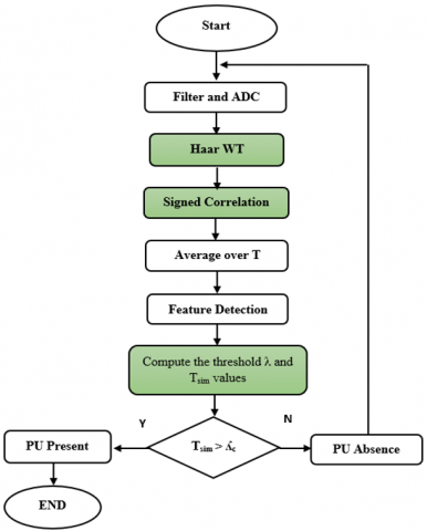
In this paper, an improved cyclostationary detection with low complexity is proposed by combining transformation and correlation processing by using a Modified Cyclostationary detector based on Haar wavelet and Signed Correlator (MCHSC). In the proposed MCHSC, the FFT process is replaced by Haar wavelet transform and the traditional autocorrelation process with the signed correlator. The two processes used to get the best reduction in the complexity of the system. Likewise, we have extracted the statistical parameter of the proposed method, named Tsim, with less complexity than the original system, and thus we have obtained a large degree of simplification of the system. The proposed system is designed for reduced complexity, time and memory the conventional system with improved performance. Figure 2 shows the structures of the proposed cyclostationary feature detectors. The highlighted blocks of the figure demonstrate the parts that are changed to lower complexity with improved performance and accuracy.
3.1 Haar wavelet transform
On changing data, the CWT solution is commonly utilized [9]. Many investigations depend on time series approach data by considering the parameters of the time series data. The time series approach is less successful due to the connection between transmission complexity and non-stationary data. Wavelet analysis, which analyzes the properties and confidence estimations of non-stationary signals, is the solution to this challenge. Wavelet analysis illustrates the frequency decomposition of a signal and determines its spectral features in time. As the Fourier transform is ineffective for analyzing time series signals with non-stationary features, a wavelet transform is invented as an improvement of the Fourier transform. The wavelet transform divides the signal into time and frequency domains. The wavelet function was first introduced by Haar. Wavelets are divided into two types, namely the written father wavelet and mother wavelet functions [12].
$\int_{-\infty}^{\infty} \emptyset(x) dx ; \int_{-\infty}^{\infty} \psi(x) d x$ (16)
Figure 2. Cyclostationary proposed detector
The Haar wavelet transform, an extension of Fourier analysis, has become widely used in various signal-processing processing technologies. Haar began with the mother function,
$\psi_{[0,1]} (r)= \begin{cases}1, & 0 \leq r<\frac{1}{2} \\ -1, & \frac{1}{2} \leq r<1 \\ 0, & \text { otherwise }\end{cases}$ (17)
To overcome the resolution problem, the continuous wavelet transform CWT was developed as an alternative method to FFT. The wavelet analyses are performed in the same manner as the FFT. More specifically, the signal is multiplied by a function (the wavelet), and the transform is performed independently for each segment of the time-domain signal. The transform is actually a convolution function-an integration of the product of the sliding wavelet function and the signal. Convolutions determine the amount of overlap between two functions as one is shifted over the other, which measures how similar they are.
The distinguishing characteristic of the wavelet transform is that the window width changes as the transform is obtained for each spectral component [13].
The continuous WT of a signal s(t) is defined as:
$C W T(a, \tau)=\int s(t) \psi^* a(t) d=1 / \sqrt{a} \int S(t) \psi^*(t-\tau / a)$ (18)
where, s(t) is the receiver signal, $\boldsymbol{\psi}^*=(\boldsymbol{t}-\boldsymbol{\tau} / \boldsymbol{a})$ is the conjugate function of the Haar function with |a| is a scaling factor that controling the width of wavelet and $\boldsymbol{\tau}$ is the translation parameter that controling the wavelet location. the scaling parameter a modifies the shape of the wavelet function. The adjustment of this parameter stretches and compresses the mother wavelet into its daughter wavelets, which changes the temporal duration of the windowing function. The scaling parameter enables the transform to have a variable window width and offers the efficiency of isolating high frequency features with good time resolution.
The factor $\frac{1}{\sqrt{a}}$ in the CWT normalizes the transform to keep the energy of the scaled wavelet the same as the energy of the mother wavelet, ψ(t), regardless of the shape and duration of the wavelet localized at time t and scaled by Martinez-Ríos et al. [14].
3.2 Signed correlator
This method is dependent on Bussgangs' theorem [15], which replaces complex multiplications with sign alterations in synthesis. This benefit, in addition to the data multiplexing process required, is further acknowledged in hardware configurations on FPGA or ASIC, where size and complexity are significantly reduced. It is known that correlation calculation can be improved by clipping one of the correlate signals to ±1, resulting in merely sign value. As a result, multiplications of the associated signal will result in sign changes of the other signal. Using Bussgang theorem, the cross correlation between two signals can be equivalent to a scaled version of one signal correlated with a transformed version of the other signal in a non-linear memory-less manner. The benefits of this kind of technique are widely known: lesser hardware, high-speed processing due to lesser logic taps, decreased storing space demands, and reduced data transmission among components of different systems.
According to Bussgang's theorem, the cross-correlation $R_{u v}(\tau)$ between u(t) and v(t) signals has the same form of function in $\tau$ as the cross-correlation $R_{u v \prime}(\tau)$ of u(t) and v(t), where $v^{\prime}(\mathrm{t})$ can be obtained from v(t) by a nonlinear memoryless transformation gave that u(t) and v(r) are stationary Gaussian processes. Let $v^{\prime}(n)$ be produced from v(n) by any nonlinear memoryless transform $\phi$[.] so that $v^{\prime}(n)=\phi[v(n)]$:
$\Phi[v]=\frac{1}{\sqrt{2}}[\operatorname{sign}(\operatorname{Re}[v])+j \operatorname{sign}(\operatorname{Im}[v])]$ (19)
Further simplification in the computation of correlation can be achieved by rotating the output of the complex sign detector by $\pi / 4$ [16]. As the rotated output of the sign detector can take one of four possible values, namely, i.e., $\mathrm{I} / \sqrt{2}$ & times (1, 0), (0, 1), (-1, 0), or (0, -1), the complex multiplications involved in correlation computation can be replaced by sign detection and multiplexing operations.
Let's consider two zero-mean complex Gaussian processes, v(n) and u(n), which are jointly stationary. Suppose $v^{\prime}(n)$ is obtained from v(n) through a nonlinear memoryless transform $\Phi[$. $]$ so that $v^{\prime}(n)=\Phi[v(n)]$. In essence, this technique simplifies the correlation computation by reducing complex multiplication to a multiplexing operation on the real and imaginary components of the input sequences. To extend the aforementioned approach of computing the time-averaged estimates of the cyclic cross spectrum let $u(n) \triangleq X_T\left(n, f_0+\right.$ $\left.\alpha_{0 / 2}\right)$ and $\mathrm{v}(n) \triangleq Y_T\left(n, f_0+\alpha_{0 / 2}\right)$. The time-averaged cyclic cross spectrum can be approximated by:
$\begin{gathered}S_{x y_T}^{\alpha_0}\left(n, f_0\right)_{\Delta t}=\frac{a\left(f_0-\alpha_0 / 2\right)}{T}\left\langle X_T\left(n, f_0+\right.\right. \left.\left.\alpha_0 / 2\right) \cdot\left(\Phi\left[Y_T\left(n, f_0-\alpha_0 / 2\right)\right] e^{j \pi / 4}\right)^*\right\rangle_{\Delta t}\end{gathered}$ (20)
where, the scaling factor is:
$\begin{gathered}a\left(f_0-\alpha_0 / 2\right) =\frac{1}{2}\left\langle\left(\Phi\left[Y_{\mathrm{T}}\left(n, f_0-\alpha_0 / 2\right)\right] e^{j \pi / 4} \cdot Y_T^*\left(n, f_0-\alpha_0 / 2\right)\right\rangle_{\Delta t}\right.\end{gathered}$ (21)
This modification, as previously mentioned, can greatly lower the computational cost of the correlation operation.
To achieve an equivalent approximate for frequencyaveraged estimations of the cross-cyclic spectrum, we notice hat for sufficiently big $\Delta t$ and little $\Delta f$, the spectral components $u(m) \triangleq X_T\left(n, f_{0+m / \Delta t}+\alpha_{0 / 2}\right)$ and $\mathrm{v}(m) \triangleq$ $Y_T\left(n, f_{0+m / \Delta t}+\alpha_{0 / 2}\right)$. Approximately statistically stationary in m throughout the averaging band of width $\Delta f$ with u(n) and v(n) substituted by u(m) and v(m). Here, the frequencyaveraged cyclic cross spectrum be approximately represented by:
$\begin{aligned} S_{x y_{\Delta t}}^{\alpha_0}\left(n, f_0\right)_{\Delta f}= & \frac{b\left(f_0-\alpha_0 / 2\right)}{\Delta t}\left\langle X_{\Delta t}\left(n, f_0+m / \Delta t\right.\right. \left.+\alpha_0 / 2\right) \cdot\left(\Phi\left[Y_{\Delta t}\left(n, f_0+m / \Delta t\right.\right.\right. \left.\left.\left.\left.-\alpha_0 / 2\right)\right] e^{j \pi / 4}\right)^*\right\rangle_{\Delta f}\end{aligned}$ (22)
where, the scaling factor is:
$\begin{aligned} b\left(f_0-\alpha_0 / 2\right)=\frac{1}{2} & \left\langle\left(\Phi\left[Y_{\Delta t}\left(n, f_0+m / \Delta t\right.\right.\right.\right. \left.\left.-\alpha_0 / 2\right)\right] e^{j \pi / 4} . Y_{\Delta t}^*\left(n, f_0+m / \Delta t\right. \left.\left.-\alpha_0 / 2\right)\right\rangle_{\Delta f}\end{aligned}$ (23)
When performed in the hardware configuration of the cyclic spectrum analyzer, the signed correlator technique offers several benefits. The hardware simplifying obtained by substituting complex multipliers used in the spectral correlation process with Signed Correlator arithmetic units is the most significant.
3.3 Threshold setting
Consequently, the sum of cyclostationary signal power at all Correlation Functions (CFs) is the sufficient statistic for the optimum detector for cyclostationary signals. This detector is called the MC detector, the total power can be calculated as:
$Y_{M C}=\sum_{k=1}^{N_\alpha} R_r^{\alpha_k}(\tau=0)$ (24)
where, $R_r^{\alpha_k}(\tau=0)$ represents the cyclostationary signal power at the kth CF.
Several ways to spectrum sensing for CR applications have been presented. The most widely considered methodologies are based on power spectrum estimation, energy detection, and multicycle cyclostationary (MC) detection. The traditional MC detector test statistic is simplified in this study to reduce computation complexity. An enhanced MC detector was suggested based on this simplification method. In comparison to the traditional detector, the suggested detector has less computational complexity with highly sensing efficiency.
Because $Y_{M C}=\operatorname{Re}\left(Y_{M C}\right)+j \operatorname{Im}\left(Y_{M C}\right)$ is a complex random variable, the traditional MC detector test statistic can be given by Zhu et al. [17].
$T_{M C}=\left|Y_{M C}\right|^2$ =$\sum_{k=1}^{N_\alpha}\left|R_r^{\alpha_k}(\tau=0)\right|^2+\sum_{k=1}^{N_\alpha} \sum_{n=1, n \neq k}^{N_\alpha} R_r^{\alpha_k}(\tau=0) R_r^{\alpha_n^*}(\tau=0)$ (25)
TMC will be simplified to lower computational complexity. Because the 2nd term of TMC requires a significant amount of computation, it is removed here. The 1st part of TMC is employed as the test statistic for the proposed detector. As a result, the simplified test statistic of the proposed detector can be defined as:
$T_{s i m}=\sum_{k=1}^{N_\alpha}\left|R_r^{\alpha_k}(\tau=0)\right|^2$ (26)
Because Tsim is the test statistic of the proposed detector, the structure of the detector can be defined as:
$T_{s i m}=\sum_{k=1}^{N_\alpha}\left|R_r^{\alpha_k}(\tau=0)\right|_{\underset{H_0}{<}}^{\stackrel{H_1}{>}} \lambda$ (27)
where, λ is the detection threshold. As a result, the suggested detector's false alarm and detecting probability can be described as:
$P_{f a}=\int_\lambda^{+\infty} P\left(T_{s i m} / H_0\right) d T_{s i m}$ (28)
$P_d=\int_\lambda^{+\infty} P\left(T_{\text {sim }} / H_1\right) d T_{\text {sim }}$ (29)
The computational complexity of TMC and Tsim can be illustrated as follows: computing TMC required N2 complex multiplication and (N2-1) complex additions. Therefore, the overall computations of TMC are (2N2-1) and thus $\theta$(N2) is the complexity of computation. For computing Tsim, we need to perform N complex multiplications and (N-1) complex additions. Thus, the total number of computations for Tsim is (2N-1), and $\theta$(N) is the computational complexity of the suggested detector.
In this section, we will demonstrate the simulation results for evaluating the performance of the proposed method that is carried out in Rayleigh flat fading channels. The simulations are performed using MATLAB version R2022b. Table 1 shows the simulation parameters used to implement the proposed method. Table 2 shows the computations complexity reduction in each stage of the proposed method in comparison with the conventional method can be noticed the amount of complexity reduction that developed in the overall system that can reach to more than 70% reduction from the conventional method with the improved performance.
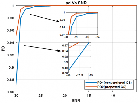
Figure 3 shows the performance of the proposed method by investigating the detection probability Pd versus SNR that show the cyclostaationay performance at low SNR ranging between −30dB and -5dB and in Rayleigh multipath flat fading channel in both conventional and proposed systems. In comparison with the conventional method, that there is an improvement in Pd which is about 0.08 in proposed method and the Pd reaches 1 at -26dB SNR in the proposed method while it is reached at -24dB in the conventional method.
Table 1. Simulation parameters used to implement the proposed approach
|
Parameter |
Value |
|
PU signal type |
QPSK |
|
Channel type |
Rayleigh flat fading |
|
Pfa |
0.01 |
|
No. of samples |
10000 |
|
SNR range |
-30 to -5dB |
Table 2. Computational complexity of each stage of the proposed and conventional methods
|
Algorithm |
Methods |
|
|
Conventional |
Proposed |
|
|
Window |
O(N) |
O(N) |
|
Frequency Transform |
O(N log2 N) |
O(N) |
|
Correlation Multiplication |
O(N2) |
O(N) |
|
Signal Detection |
2*O(N2)+O(N) |
O(N2)+O(N) |
|
Total |
2*O(N)+2*O(N2)+O(N LOG N) |
4*O(N)+O(N2) |
Figure 3. The performance comparison of conventional and suggested methods corrupted by Rayleigh & AWGN channel
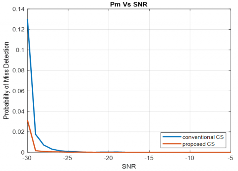
Figure 4. The miss detection probability with SNR comparison of conventional and proposed method
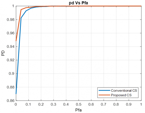
Figure 5. The detection performance with Pfa comparison of conventional and proposed method
Figure 6. The performance comparison of conventional and proposed approach number in terms of the number of samples regarding to computational complexity ratio
Figure 4 shows the plot of SNR versus Pm with a fixed Pfa=0.01. As shown, a lower probability of missed detection can be achieved using the proposed method than conventional method.
Figure 5 illustrates the relationship between Pfa and Pd at SNR value of -30dB. This curve indicates that as Pfa increases, the Pd also increases. Furthermore, it is observed that the detection probability reaches its maximum value of Pd=1 when the false-alarm probability exceeds 0.1, with the proposed method Pfa equal 0.2 in conventional method.
Figure 6 demonstrates comparison of traditional and proposed methods by investigating the number of samples versus the computational complexity ratio. It can be seen in this figure that the computing complexity is significantly reduced using the proposed MCHSC method as compared to traditional method and this reduction is increased as the number of samples is increased. For instance, the computational complexity of conventional cyclostationary and proposed technique methods are computed as shown in the following equations [9]:
$C_{C S}=C_w+C_{f t}+C_{\text {Corr }}+C_{s d}$ (30)
where, CCS=total computational complexity of cyclostationary technique, Cw=Widowing complexity, Cft=Fourier transform complexity and Csd=Signal Detection complexity
In conventional cyclostationary, computational complexity Cconv is computed as follows:
$C_{\text {conv }}=N+N \log 2 N+N 2+N 2+N=2 N+2 N 2+N \log 2 N$ (31)
In the proposed, the computational complexity Cprop are computed as follows:
$C_{\text {prop }=}=N+N+N+N 2+N=4 N+N 2$ (32)
The computational complexity ratio of each method is computed as follows:
$C_{\text {conv }}$ ratio $=C_{\text {conv }} / C_{\text {conv_max }}$ (33)
$C_{\text {prop }}$ ratio $=C_{\text {prop }} / C_{\text {conv_max }}$ (34)
Cconv_max=maximum computational complexity of conventional method.
Table 3 shows comparison between proposed and other studies in terms of the average complexity reduction, number of samples, probability of false alarm and probability of detection. The table shows that the proposed method is better in complexity reduction, probability of detection and in lower SNR values.
Table 3. Performance of the proposed method compared with previous implementations
|
Method |
SNR |
Pfa |
Pd |
N |
Complexity Reduction |
|
[18] |
-20 |
-- |
0.5 |
32 |
40% |
|
[9] |
0 to 10 |
0.001 |
0.7 |
100 |
40% |
|
[19] |
-20 to 0 |
0.1 |
0.1 |
8 |
70% |
|
[20] |
-20 to 0 |
0.1 |
0.8-0.9 |
1000 |
40% |
|
Proposed Method |
-30 to -5 |
0.01 |
0.95 |
10000 |
>70% |
Table 4. Proposed system performance in terms of complexity cost, time, and storage compared with a conventional system
|
Method |
Avg Complexity Reduction (%) |
Time(s) |
Storage (MB) |
|
Conventional |
- |
1.203 |
4169 |
|
Proposed |
⁓70% |
0.46 |
3855 |
Table 4 shows comparison between proposed and conventional methods in terms of the average complexity reduction, time and required storage. The table shows that the proposed system significantly improves all above mentioned parameters at low SNR reach to -30 with reduction >70% in complexity, 60% in time, and 7% in memory storage, with improved detection performance that is about 8% compared to conventional method.
Cyclostationary feature detection can be computationally intensive as the cyclostationary features may require significant computationally resources making real-time processing challenging, particularly in resource constrain environments. In this research, a low-complexity cyclostationary feature detection for improved primary user signal detection with reduced computational complexity is proposed. The proposed detection method uses Haar wavelet transform and signed correlator with simplified test statistics for digital communication receivers with QPSK Modulation. The proposed detection is computationally effective and can be easily implemented using embedded systems, signal classification and modulation recognition for practical application. The complexity reduction is also referred to that the proposed signed correlator algorithm only takes the sign bit of the real and imaginary portions of spectral data, so the storage and transfer issues are considerably minimized. The simulation result shows that the proposed method significantly reduces the complexity cost, time, and storage at low SNR reaches -30dB with reduction >70% in complexity, 60% in time, and 7% in memory storage, with improved detection performance that is about 8% compared to conventional method.
The system is evaluated under an AWGN and Rayleigh multipath fading. Other effects like other fading types, Doppler shift, phase error, etc., can be added to the channel in order to closely reflect the real-life system. The utilization of the Multiple Input Multiple Output (MIMO) technique can enhance the results of cyclostationary feature detection. Additionally, cooperative communication can be employed to sense the spectrum, taking into account factors such as antenna diversity and other relevant considerations. These approaches contribute to improved cyclostationary feature detection outcomes.
[1] Hamed, I., Elmenyawi, M.A., Hassan, A.Y. (2021). Comparative study between cognitive radio techniques in FM broadcasting band. In IOP Conference Series: Materials Science and Engineering. IOP Publishing, 1172(1): 012009. http://doi.org/10.1088/1757 899x/1172/1/012009
[2] Yawada, P.S., Wei, A.J. (2016). Cyclostationary detection based on non-cooperative spectrum sensing in cognitive radio network. In 2016 IEEE International Conference on Cyber Technology in Automation, Control, and Intelligent Systems (CYBER), Chengdu, China, pp. 184-187. http://doi.org/10.1109/CYBER.2016.7574819
[3] Gao, Y.L., Chen, Y.P. (2009). Modification and digital implementation of fam algorithm for spectral correlation. In 2009 International Conference on Wireless Communications & Signal Processing, Nanjing, China, pp. 1-4. https://doi.org/10.1109/WCSP.2009.5371440
[4] Zhang, X., Zhang, Y., Liu, C., Jia, H. (2018). Low-complexity detection algorithms for spatial modulation MIMO systems. Journal of Electrical and Computer Engineering, 2018: 1-7. https://doi.org/10.1155/2018/4034625
[5] Hu, Y., Yu, B., Deng, Z., He, G., Zhou, H. (2019). Efficient cycle frequency acquisition of a cyclostationary signal with the FACA method. Radioengineering, 28(2): 447-455. http://doi.org/10.13164/re.2019.0447.
[6] Souza, P., Souza, V., Silveira, L.F. (2019). Analysis of spectral sensing using angle-time cyclostationarity. Sensors, 19(19): 4222. https://doi.org/10.3390/s19194222
[7] Kadjo, J.M., Agoua, R., Bamba, A., Konaté, A., Asseu, O. (2021). Non-cooperative spectrum sensing based on cyclostationary model of digital signals in the context of cognitive radio. Engineering, 13(01): 56. http://doi.org/10.4236/eng.2021.131005
[8] Mathew, S.G., Samuel, C.P. (2021). A novel low-complexity cyclostationary feature detection using sub-nyquist samples for wideband spectrum sensing. Circuits, Systems, and Signal Processing, 40: 6371-6386. https://doi.org/10.1007/s00034-021-01771-0
[9] Abdullah, H.N., Dawood, Z.O., Abdelkareem, A.E., Abed, H.S. (2020). Complexity reduction of cyclostationary sensing technique using improved hybrid sensing method. Acta Polytech, 60(4): 279-287. http://doi.org/10.14311/AP.2020.60.0279
[10] Arjoune, Y., Kaabouch, N. (2019). A comprehensive survey on spectrum sensing in cognitive radio networks: Recent advances, new challenges, and future research directions. Sensors, 19(1): 126. https://doi.org/10.3390/s19010126
[11] Spooner, C.M. (1992). Theory and application of higher-order cyclostationarity. University of California, Davis, 29(2): 229. http://doi.org/10.1016/0165-1684(92)90027-T
[12] Nugroho, L.W., Saputro, D.R.S. (2022). Signal analysis with continuous wavelet transform. In AIP Conference Proceedings. AIP Publishing, 2577(1). http://doi.org/10.1063/5.0096025
[13] Ali, A., Sheng-Chang, C., Shah, M. (2020). Continuous wavelet transformation of seismic data for feature extraction. SN Applied Sciences, 2: 1-12. https://doi.org/10.1007/s42452-020-03618-w
[14] Martinez-Ríos, E.A., Bustamante-Bello, R., Navarro-Tuch, S., Perez-Meana, H. (2022). Applications of the generalized Morse wavelets: A review. IEEE Access, 11: 667-688. http://doi.org/10.1109/ACCESS.2022.3232729
[15] Gardner, W.A., Roberts, R.S. (1993). One-bit spectral-correlation algorithms. IEEE Transactions on Signal Processing, 41(1): 423. http://doi.org/10.1109/TSP.1993.193170
[16] Jacovitti, G., Neri, A., Cusani, R. (1987). Methods for estimating the autocorrelation function of complex Gaussian stationary processes. IEEE Transactions on Acoustics, Speech, and Signal Processing, 35(8): 1126-1138. http://doi.org/10.1109/TASSP.1987.1165253
[17] Zhu, Y., Liu, J., Feng, Z., Zhang, P. (2014). Sensing performance of efficient cyclostationary detector with multiple antennas in multipath fading and lognormal shadowing environments. Journal of Communications and Networks, KICS, 16(2): 162-171. http://doi.org/10.1109/JCN.2014.000027
[18] Chaiel, H.K. (2015). Analysis of cyclostationary CR detector for OFDM signals. University of Thi-Qar Journal for Engineering Sciences, 6(1): 100-120.
[19] Cho, D., Narieda, S., Umebayashi, K. (2018). Low computational complexity spectrum sensing based on cyclostationarity for multiple receive antennas. IEICE Communications Express, 7(2): 54-59. https://doi.org/10.1587/comex.2017XBL0167
[20] Shrestha, R., Telgote, S.S. (2020). A short sensing-time cyclostationary feature detection based spectrum sensor for cognitive radio network. In Proceedings- IEEE International Symposium on Circuits and Systems, Seville, Spain, pp. 1-5. http://doi.org/10.1109/iscas45731.2020.9180415