Jairo J. Marquina-Araujo*![]() | Marco A. Cotrina-Teatino
| Marco A. Cotrina-Teatino![]() | José N. Mamani-Quispe
| José N. Mamani-Quispe![]() | Johnny H. Ccatamayo-Barrios
| Johnny H. Ccatamayo-Barrios![]() | Salomon M. Ortiz-Quintanilla
| Salomon M. Ortiz-Quintanilla![]() | Eusebio Antonio-Araujo
| Eusebio Antonio-Araujo![]() | Aldo R. Castillo-Chung
| Aldo R. Castillo-Chung![]() | Hans R. Portilla-Rodriguez
| Hans R. Portilla-Rodriguez![]()
© 2024 The authors. This article is published by IIETA and is licensed under the CC BY 4.0 license (http://creativecommons.org/licenses/by/4.0/).
OPEN ACCESS
The primary aim of this research was to delimitate the final pit in an open pit mine using the 1×5 and 1×9 arch methods of the pseudoflow maximum flow algorithm. To achieve this, Exploratory Data Analysis (EDA), economic, and geomechanical parameters were utilized. Various final pit scenarios were generated by varying the revenue factor. The analysis was conducted using Python 3.11 (Jupyter Notebook) and SGeMS V.3.0 software. The block model comprised 480,000 blocks, each measuring 10×10×10 meters, with a copper grade range from 0 to 1.41%. Specific parameters were employed, including a slope angle of 45°, a base copper price of 3.90 US\$/lb, and smelting, extraction, and crushing-grinding costs of 0.40 US\$/lb, 2.30, and 11.00 US\$/ton, respectively. Twenty final pits were generated for each method, based on a revenue factor from 0.10 to 2.00. The results indicated that both methods are effective for final pit delineation, with the 1×5 method achieving an NPV of 17,855 MUS\$ and a REM of 0.27, and the 1×9 method attaining an NPV of 18,456 MUS$ and a REM of 0.35. It was concluded that the 1×9 arch method is preferable as it yields a higher NPV. This study underscores the importance of methodological selection in the planning of open-pit mines, demonstrating that despite a higher REM, the 1×9 method significantly enhances the NPV, implying substantial economic benefits for the industry.
final pit, Net Present Value, pseudoflow, arcs
In the challenging context of open-pit mining, this study focuses on the application of the 1×5 and 1×9 arch methods of the pseudoflow algorithm, providing a detailed analysis of their efficiency and accuracy in optimally delimiting the boundaries of the mines. The open-pit mining technique, widely employed in mineral exploitation, is characterized by the use of pits or "pits" [1]. Before commencing any mining operation, it is vitally important to precisely design the outline and final boundaries of the extraction zone [2]. Current practices in open-pit mining involve a variety of methods and algorithms to design the outline and final boundaries of the extraction zone. These methods consider a series of fundamental factors such as the geology and topography of the site [3], the distribution of minerals, geotechnical restrictions, and slope stability [4, 5], environmental considerations, extraction, and processing costs [6], metallurgical recovery [7], and the price of minerals [8].
However, these methods often face limitations [9]. For instance, heuristic algorithms like the floating cone and its improvements, Korobov, Boykov-Kolmogorov, and Ford Fulkerson, do not guarantee mathematically optimal solutions. This represents a significant limitation in current practice. Similarly, the use of the Lerchs-Grossman algorithm can result in prolonged execution times when applied to a block model with a large amount of data. The main goal of this design in open-pit mining is to establish, prior to operations, the definitive layout, and dimensions of the mine, considering a series of fundamental factors. Such factors encompass the geology and topography of the site, the distribution of minerals, geotechnical restrictions, and slope stability [9], environmental considerations, extraction and processing costs, metallurgical recovery, and the price of minerals.
In this scenario, the pseudoflow algorithm emerges as an effective tool for overcoming these limitations. The pseudoflow algorithm employs an optimality certificate based on the Lerchs and Grossman algorithm for the maximum cut problem in a graph of weighted nodes. This approach shows that the concept of mass can be generalized to capacity networks using the notion of pseudoflow. Unlike the maximum flow problem, the pseudoflow addresses the maximum blocking cut problem, focused on the capacities of the arches and the weights of the nodes, without considering source and destination nodes. Its goal is to find a subset of nodes that maximize the blocking cut.
The definition of the final boundaries of the mine plays a crucial role in the design of open-pit mining operations. To achieve this precise definition, block models are used that represent the reserve through the combination of small blocks, using inverse distance or geostatistical methods [5]. In recent decades, two main approaches have been proposed to establish the final contour: the maximization of undiscounted benefit and the maximization of Net Present Value (NPV). Each approach has specific methods and algorithms. The first approach seeks to maximize the non-discounted benefit by initially establishing the boundaries of the mine. Subsequently, the production schedule is planned to obtain the highest NPV. Among the most used heuristic algorithms are the floating cone [10] and its improvements [11], Korobov [12], Boykov-Kolmogorov [13], and Ford Fulkerson [14]. However, these algorithms do not guarantee mathematically optimal solutions.
Muir [15] conducted a comprehensive study on the optimization of open pit mine pits using the Lerchs-Grossmann (LG) algorithm and its evolution to pseudoflow flow models. Implemented and compared four methods based on the LG algorithm, including Hochbaum's lowest and highest label pseudoflow variants, on three different ore properties. The results obtained indicated that the pseudoflow variants, especially when using priority queues, are significantly faster and reduce the number of merges and prunings required to reach optimality. In addition, the same optimal Net Present Value (NPV) value was maintained for the mine. On the other hand, Morrison [16] presented a detailed discussion on the application of the pseudoflow algorithm to solve maximum blockage cut-off and minimum residue flow problems. Through linear and combinatorial programming methods, he demonstrated how these problems, which are applicable in contexts such as open-pit mining, can be solved simultaneously with the pseudoflow algorithm. This approach proved to be efficient and theoretically sound. Bai et al. [17] conducted a performance comparison between the pseudoflow algorithm and the LG algorithm in open pit mining pit optimization. The results highlighted a significant reduction in computational time when using pseudoflow compared to LG, with especially noticeable improvements in large block models. For example, in the case of 21.3 million blocks, the time was reduced from 15 hours to just 12 minutes. Musenge et al. [14] explored the application of the Ford and Fulkerson algorithm to optimize the final boundaries of an open pit mine. Implemented in Python, the algorithm proved to be effective in defining the final mine boundaries in three dimensions through two-dimensional sections. Comparing the results with the LG algorithm, the Ford Fulkerson peak flow algorithm managed to design the optimal mine boundary in record time, offering optimal pit values with minimal difference in Net Present Value (NPV), being USD 881870000 for FFA and USD 880210100 for LG. Finally, Chicoisne et al. [18] indicated that there are open-source implementations of the pseudoflow algorithm, such as MineFlow, that provide efficient precedence schemes and a simplified pseudoflow-based solver.
The Lerchs-Grossman (LG) algorithm [19], based on graph theory, and the network flow algorithm [20] also determine the final boundaries of the pit using mathematical approaches. Each method has its pros and cons. For example, the use of the Lerchs-Grossman algorithm to obtain optimal pit boundaries, when applied to a block model with a large amount of data, can result in prolonged execution times [21]. The maximum flow problem seeks to maximize the amount of flow that can pass from a source to a destination in a network with capacities on the arches. To solve this problem, two types of algorithms have been developed: feasible flow algorithms, which increase the flow in each iteration using augmenting paths, and preflow algorithms, which allow excesses in the flow balance [22]. The first feasible flow algorithm was proposed by Ford and Fulkerson in 1957, while the first known use of preflows was in 1955 by Boldyreff [23]. However, this technique did not guarantee optimal solutions. The Push-relabel algorithm by Goldberg and Tarjan from 1988 [24, 25] uses preflows and has proven to be efficient both theoretically and in practice.
In this scenario, the pseudoflow algorithm emerges as an effective tool for determining the final boundaries of the contour in open-pit mining. The pseudoflow algorithm employs an optimality certificate based on the Lerchs and Grossman algorithm for the maximum cut problem in a graph of weighted nodes. This approach shows that the concept of mass can be generalized to capacity networks using the notion of pseudoflow [22]. Unlike the maximum flow problem, the pseudoflow addresses the maximum blocking cut problem, focused on the capacities of the arches and the weights of the nodes, without taking into account source and destination nodes. Its goal is to find a subset of nodes that maximizes the sum of the weights of the nodes minus the capacities of the arches leaving the subset [24]. The pseudoflow algorithm stands out as an optimal and efficient solution to determine the final contour of an open pit mine. This research paper will delve into the development, implementation, and results obtained with the 1×5 and 1×9 arch methods of the pseudoflow algorithm to define the final boundaries of the contour in open-pit mining.
This research introduces an innovative comparative analysis of geometric precedence constraints with 1×5 and 1×9 arcs in the application of the pseudoflow algorithm for final pit delimitation in open pit mining.
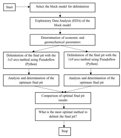
A study has been carried out in a surface mine located in southern Peru in order to validate the final pit delimitation methods. A logic scheme is presented showing how the final pit delimitation process looks like, applying the 1×5 and 1×9 arcs methods of the maximum pseudoflow algorithm.
2.1 Database information
The database used in this study comprised 480,000.0 blocks organized into 10 distinct columns. These columns included critical information such as the spatial coordinates (x, y, z) determining the block's location; dimensions along the x, y, z axes; the copper grade percentage (Cu); the volume measured in cubic meters (m3); the density expressed in tons per cubic meter (t/m3); and the calculated tonnage for each block (t). Table 1 shows the characteristics of the first ten blocks within this database. For example, block number 1 is characterized by having coordinates x=10,305; y=10,305 and z=3,555, with uniform dimensions of 10×10×10 meters along all axes. Moreover, this block exhibits a copper grade of 0.37%, a volume of 1000 m3, a density of 2.30 t/m3, and a tonnage of 2300 tons. Figure 1 shows a summary of the methodology used in the research.
2.2 Validation of the block model
To validate the block model, tests and comparisons were made on data from a specific open pit mine located in southern Peru. The model blocks were compared with mine sampling data to verify the accuracy of coordinates, block dimensions, copper percentage, volume, and density. Although specific mine details are kept confidential for privacy reasons, the validation results confirmed that the block model provides an accurate representation of actual mine conditions.
2.3 Exploratory Data Analysis
Exploratory Data Analysis (EDA) is a set of procedures that researchers follow to understand the overall structure of the data, identifying anomalies, and gaining insights that can be used in more complex analyses. Exploratory Data Analysis encompasses techniques such as: the generation of summary statistics, the creation of data graphs (histograms, scatter plots), the identification of correlations between variables [25-28].
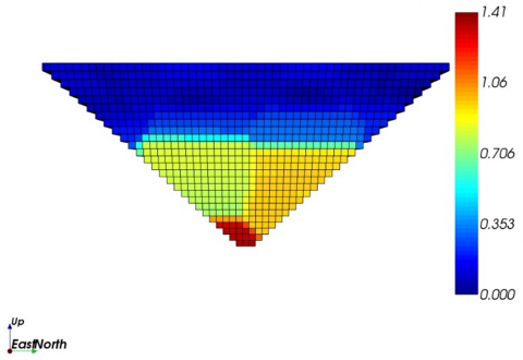
In this research, an Exploratory Data Analysis (EDA) was conducted to explore the distribution of copper ore grade within the block model, as depicted in Figure 2. It was found that the copper ore grade ranges from a minimum of 0.00% to a maximum of 1.41%.
Figure 1. Methodology overview
Table 1. Block model database
|
X |
Y |
Z |
Dim X (m) |
Dim Y (m) |
Dim Z (m) |
Cu (%) |
Vol (m3) |
Density (t/m3) |
Tonnage (t) |
|
1 |
10,305 |
10,305 |
3,555 |
10 |
10 |
10 |
0.37 |
2.3 |
2,300 |
|
2 |
10,315 |
10,305 |
3,555 |
10 |
10 |
10 |
0.39 |
2.3 |
2,300 |
|
3 |
10,325 |
10,305 |
3,555 |
10 |
10 |
10 |
0.42 |
2.3 |
2,300 |
|
4 |
10,335 |
10,305 |
3,555 |
10 |
10 |
10 |
0.40 |
2.3 |
2,300 |
|
5 |
10,345 |
10,305 |
3,555 |
10 |
10 |
10 |
0.40 |
2.3 |
2,300 |
|
6 |
10,355 |
10,305 |
3,555 |
10 |
10 |
10 |
0.40 |
2.3 |
2,300 |
|
7 |
10,365 |
10,305 |
3,555 |
10 |
10 |
10 |
0.39 |
2.3 |
2,300 |
|
8 |
10,375 |
10,305 |
3,555 |
10 |
10 |
10 |
0.39 |
2.3 |
2,300 |
|
9 |
10,385 |
10,305 |
3,555 |
10 |
10 |
10 |
0.39 |
2.3 |
2,300 |
|
10 |
10,395 |
10,305 |
3,555 |
10 |
10 |
10 |
0.37 |
2.3 |
2,300 |
Figure 2. Cooper grades in the block model
The geometric parameters of the model are shown in the Table 2, indicating that the model consists of 486,000 blocks. Each block's dimensions, in its east (x), north (y), and elevation (z) coordinates, are 10 meters, with a density of 2.30 t/m3, resulting in a tonnage of 2300.00 tons per block.
Table 2. Parameters of the block model
|
Length x (m) |
Length y (m) |
Length z (m) |
Density (ton/m3) |
Tonnage (Ton) |
Total Blocks |
|
10.00 |
10.00 |
10.00 |
2.30 |
2300.0 |
486000 |
Table 3 presents a summary of the block model statistics, showing the minimum, maximum, and average coordinates in the east, north, and elevation axes, as well as the minimum, maximum, and average values for copper grade, volume (m3), and density (tons/m3).
Table 3. Block model statistics
|
Description |
Min |
Max |
Average |
|
Coordinate (x) |
10305.00 |
11195.00 |
10750.00 |
|
Coordinate (y) |
10305.00 |
11195.00 |
10750.00 |
|
Coordinate (z) |
3555.00 |
4145.00 |
3850.00 |
|
Copper grade (%) |
0.00 |
1.41 |
0.33 |
|
Volume (m3) |
1000.00 |
1000.00 |
1000.00 |
|
Density (t/m3) |
2.3 |
2.3 |
2.3 |
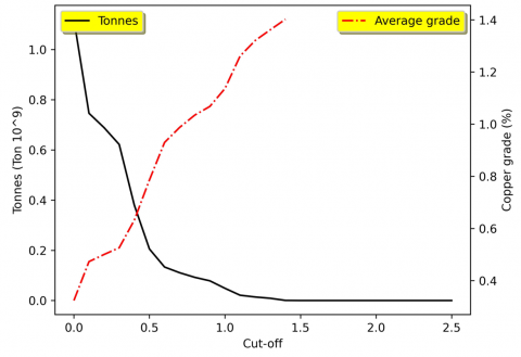
For a more detailed analysis, a tonnage versus average grade curve was constructed, revealing an intersection between the two curves. This intersection indicates that higher tonnage corresponds to a lower percentage of copper ore grade, as illustrated in Figure 3.
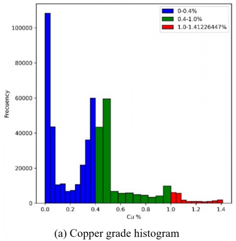
According to Figure 4, which displays the histogram of copper grades and lithologies, the copper grades are divided into three categories: low (blue), medium (green), and high (red). A total of 315,895.00 blocks had a low copper grade (between 0.00% and 0.40%), 1,482,214.00 blocks had a medium copper grade (between 0.40% and 1.00%), and 21,891.00 blocks had a high copper grade (between 1.00% and 1.42%). Regarding lithologies, 112,486.00 blocks were classified under lithologic code 1, 243,267.00 blocks under lithologic code 2, and 130,247 blocks under lithologic code 3, resulting in a total of 486,000.00 blocks.
Figure 3. Tonnes vs. grade curve
Figure 4. Frequency histograms
2.4 Delimitation of the final pit with pseudoflow method
The pseudoflow algorithm, which is used to resolve the final pit in mining, operates iteratively and has certain advantages over the Lerchs and Grossman algorithm. Unlike the latter, the pseudoflow algorithm uses the idea of flow rather than mass, facilitating the efficient update of different structures [17]. A pseudoflow is a type of relaxed flow that does not require nodes to comply with flow balance constraints. Nodes may have an excess of inflows over outflows or a deficit of these. The numbers on the arcs indicate the current flow through each arc, while the numbers inside the nodes represent the current surpluses or shown in references [5, 29-32].
The bounding problem is formulated to maximize the Net Present Value of the extracted materials, constrained by the flow capacities of each block and the overall system, ensuring that the solution adheres to the operational and geotechnical constraints. The objective function and constraints are mathematically expressed as follows: Maximize the total flow Z from source to sink [3]:
$\mathrm{Z}=\sum_{(s, i) \in E} F_{s i}$ (1)
Subject to capacity constraints on each edge $(i, j)$:
$\mathrm{F}_{i j} \leq C_{i j} \quad \forall(i, j) \in E$ (2)
Ensure flow conversation at each node, except at the source and sink:
$\sum_{(i, j) \in E} F_{i j}-\underset{\in V \backslash\{{ source }, sin k\}}{\sum_{(j, i) \in E} F_{i j}=0 \forall i}$ (3)
Non-negativity of the flow:
$F_{i j} \geq 0 \quad \forall(i, j) \in E$ (4)
In addition, 1×5 and 1×9 arch constraints allow accurate modeling of slope angles for final pit planning. These constraints are implemented by defining arcs with capacities that represent the economic and geomechanical costs associated with the extraction of adjacent blocks, adapting the flow model to the complexity and specific constraints of the mine site.
The economic parameters used in the delimitation of the final pit included: cost of sale $\left(C_v\right)$ which represents the cost associated with the sale of the extracted ore, including transportation and marketing. Processing cost $\left(C_p\right)$ which includes expenses related to the transformation of the ore into saleable product, such as crushing, grinding and flotation. Mining cost $\left(C_m\right)$ which encompasses the direct operating costs of mining. Ore price $(P)$ which is the market value per unit of ore mined. Metallurgical recovery $(y)$ which is the percentage of metal recovered in the processing process. Average grade $(g)$ which is the average concentration of the metal of interest in the ore. Ore tonnage $\left(T_m\right)$ and total tonnage $\left(T_t\right)$ which represents, the mass of ore containing the metal of interest and the total mass mined including tailings, respectively. A profit factor $(\alpha)$. The block profitability $(B E)$ is calculated with the formula [33]:
$\mathrm{BE}=\mathrm{T}_{\mathrm{m}} *\left(\mathrm{~g} * \mathrm{y} *\left(\mathrm{P} * \alpha-\mathrm{C}_{\mathrm{v}}\right)-\mathrm{C}_{\mathrm{p}}\right)-\mathrm{T}_{\mathrm{t}} * \mathrm{C}_{\mathrm{m}}$ (5)
Specific details of these economic and operational parameters applied in the study, including numerical values for copper price, processing costs, metallurgical recovery, mining cost and crushing and milling costs are presented in Table 4.
Table 4. Economic and operational parameters
|
Economic and Operational Parameters |
Quantity |
Units |
|
Cooper price (P) |
3.9 |
US$/lb |
|
Processing cost (Cp) |
0.4 |
US$/lb |
|
Metallurgical recovery (y) |
90 |
% |
|
Mine cost (Cm) |
3.5 |
US$/t |
|
Crushing and grinding cost (Cg) |
11 |
US$/t |
Table 5 presents the geomechanical parameters used in the study, which used 1×5 and 1×9 arch constraints to accurately model the slope angles, which were set at 45° for both types of arches.
Table 5. Geomechanical parameters
|
Description |
Arches 1×5 |
Arches 1×9 |
|
Slope angle |
45° |
45° |
The modeling of the extraction sequence is carried out through the conceptualization of the slope angle, using the principle of precedence: block "A" precedes another block "B" if the extraction of B requires the previous removal of A. This precedence relationship between blocks is transitive, that is, if "A" is a predecessor of "B", and "B" is a predecessor of "C", then "A" also precedes "C". Consequently, a tree of precedences is generated. The transitivity of this condition culminates in defining a rigorous order in which the extraction process must be carried out. That is, if a specific block is planned to be extracted, the extraction order must be such that all the blocks that precede it are extracted first [34-36]. There are various strategies to define the precedence arcs in an open-pit mining operation, of which the most common are: Definition of a classic 5-block mold (1×5 arcs): this strategy seeks to specifically represent a 45° angle. Its use is recommended when the block dimensions are homogeneous so that the interpretation fits this circumstance as shown in Figure 5.
Figure 5. 1×5 arc model
Definition of a fixed 9-block mold (1×9 arcs): this strategy also aims to represent a 45° angle, but with greater amplitude. Like the previous strategy, its application is recommended in situations where the block dimensions are homogeneous for a proper interpretation as shown in Figure 6.
Figure 6. 1×9 arc model
To carry out the final pit delimitation in open pit mines, it is very important to consider economic, operational and geomechanical parameters already detailed above.
Applying the 1×5 arc methodology and using a revenue factor ranging from a minimum of 0.1 to a maximum of 2 with an increment of 0.1, generated 20 final pits of different tonnages, NPV and ore grade, as shown in Table 6. Similarly, Figure 7 shows the visualization of the pit 1 scenario when applying the 1×5 arc methodology.
Table 6. Multiple final pit scenarios generated with the application of 1×5 arcs
|
Pit |
Ore (Mt) |
Waste (Mt) |
Total Tonnage (Mt) |
NPV (MUS$) |
REM |
Ore Grade (%) |
Revenue Factor |
|
1 |
47.35 |
70.35 |
117.69 |
232.95 |
1.49 |
0.50 |
0.10 |
|
2 |
98.40 |
78.31 |
176.70 |
940.59 |
0.8 |
0.46 |
0.20 |
|
3 |
121.30 |
77.53 |
198.84 |
1765.34 |
0.64 |
0.44 |
0.30 |
|
4 |
136.94 |
78.37 |
215.31 |
2638.74 |
0.57 |
0.43 |
0.40 |
|
5 |
147.52 |
79.26 |
226.78 |
3541.65 |
0.54 |
0.42 |
0.50 |
|
6 |
155.51 |
77.97 |
233.48 |
4462.16 |
0.50 |
0.41 |
0.60 |
|
7 |
163.05 |
76.43 |
239.49 |
5393.08 |
0.47 |
0.40 |
0.70 |
|
8 |
172.07 |
71.92 |
243.99 |
6331.58 |
0.42 |
0.40 |
0.80 |
|
9 |
181.13 |
68.94 |
250.07 |
7276.58 |
0.38 |
0.39 |
0.90 |
|
10 |
193.07 |
66.35 |
253.89 |
8226.82 |
0.35 |
0.39 |
1.00 |
|
11 |
197.66 |
64.37 |
257.45 |
9181.37 |
0.33 |
0.38 |
1.10 |
|
12 |
200.89 |
63.09 |
260.75 |
10139.20 |
0.32 |
0.38 |
1.20 |
|
13 |
204.07 |
60.80 |
261.68 |
11099.59 |
0.30 |
0.38 |
1.30 |
|
14 |
206.07 |
60.61 |
264.68 |
12062.01 |
0.30 |
0.38 |
1.40 |
|
15 |
207.89 |
60.11 |
266.18 |
13025.18 |
0.29 |
0.37 |
1.50 |
|
16 |
209.08 |
59.56 |
267.45 |
13990.29 |
0.29 |
0.37 |
1.60 |
|
17 |
210.42 |
59.12 |
268.20 |
14955.55 |
0.28 |
0.37 |
1.70 |
|
18 |
211.39 |
59.58 |
270.00 |
15921.88 |
0.28 |
0.37 |
1.80 |
|
19 |
211.39 |
58.61 |
270.00 |
16888.84 |
0.28 |
0.37 |
1.90 |
|
20 |
212.34 |
58.36 |
270.69 |
17855.97 |
0.27 |
0.37 |
2.00 |
Figure 7. Scenario of pit 1 applying 1×5 arcs
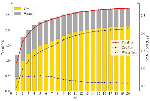
In Figure 8, a pit-by-pit graph generated with 1×5 arches is observed, showing that each pit has its determined tonnage of ore and waste, as well as its total tonnage, tons of ore and tons of waste. This graph has two y-axes (y-left) where the total tonnage is placed, and on the y-right axis, the NPV (Net Present Value) is shown in dollars.
Figure 8. Pit by pit graph when applying 1×5 arcs
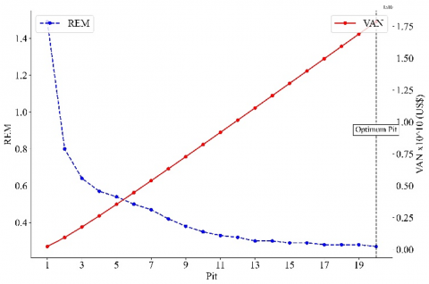
Figure 9. REM vs. VAN graph when applying 1×5 arcs
In Figure 9, the REM vs. NPV graph for the final pit using 1×5 arches is shown. It can be seen that the optimal final pit is pit 20, as it has a higher NPV (Net Present Value) and a lower REM (Waste-Ore Ratio). In this case, the NPV was 17,856 MUS$ and the REM was 0.27, indicating that 0.27 tons of waste will be extracted for every ton of ore.
By applying the 1×9 arch methodology and using a revenue factor that ranged from a minimum of 0.10 to a maximum of 2.00 with an increment of 0.10, it generated 20 final pits of different tonnages, NPV and ore grade, as observed in Table 7. Similarly, Figure 10 shows the visualization of the pit 1 scenario when applying the 1×9 arc methodology.
Figure 10. Scenario of pit 1 applying 1×9 arcs
Figure 11. Pit by pit graph when applying 1×9 arches
Figure 12. REM vs. VAN graph when applying 1×9 arches
In Figure 11, a pit-by-pit graph generated with 1×9 arches is observed, showing that each pit has its determined tonnage of ore and waste, as well as its total tonnage, tons of ore and tons of waste. This graph, its values are in relation to the Net Present Value (NPV) in dollars.
In Figure 12, the REM vs. NPV graph for each final pit using 1×9 arches is shown. The optimal final pit is pit 20, as it has a higher NPV and a lower REM, with the NPV being 18,456.47 MUS$ and a REM of 0.35, which means that 0.35 tons must be extracted for each ton of ore.
Table 7. Multiple final pit scenarios generated with the application of 1×9 arcs
|
Pit |
Ore (Mt) |
Waste (Mt) |
Total Tonnage (Mt) |
NPV (MUS$) |
REM |
Ore Grade (%) |
Revenue Factor |
|
1 |
21.80 |
36.86 |
58.66 |
272.86 |
1.69 |
0.45 |
0.10 |
|
2 |
70.44 |
88.02 |
158.46 |
1104.09 |
1.25 |
0.40 |
0.20 |
|
3 |
131.09 |
121.20 |
252.29 |
2294.02 |
0.92 |
0.36 |
0.30 |
|
4 |
156.86 |
127.21 |
284.07 |
3360.29 |
0.81 |
0.35 |
0.40 |
|
5 |
164.77 |
124.07 |
288.83 |
4290.84 |
0.75 |
0.35 |
0.50 |
|
6 |
170.14 |
118.70 |
288.83 |
5196.71 |
0.70 |
0.35 |
0.60 |
|
7 |
175.61 |
113.23 |
288.83 |
6111.36 |
0.64 |
0.35 |
0.70 |
|
8 |
182.78 |
106.05 |
288.83 |
7035.32 |
0.58 |
0.35 |
0.80 |
|
9 |
189.32 |
99.51 |
288.83 |
7968.33 |
0.53 |
0.35 |
0.90 |
|
10 |
194.34 |
94.50 |
288.83 |
8908.24 |
0.49 |
0.35 |
1.00 |
|
11 |
198.66 |
90.17 |
288.83 |
9853.22 |
0.45 |
0.35 |
1.10 |
|
12 |
202.15 |
86.68 |
288.83 |
10802.21 |
0.43 |
0.35 |
1.20 |
|
13 |
205.21 |
83.63 |
288.83 |
11754.17 |
0.41 |
0.35 |
1.30 |
|
14 |
207.41 |
81.43 |
288.83 |
12708.50 |
0.39 |
0.35 |
1.40 |
|
15 |
208.96 |
79.88 |
288.83 |
13664.31 |
0.38 |
0.35 |
1.50 |
|
16 |
210.39 |
78.44 |
288.83 |
14621.32 |
0.37 |
0.35 |
1.60 |
|
17 |
211.38 |
77.46 |
288.83 |
15579.19 |
0.37 |
0.35 |
1.70 |
|
18 |
212.22 |
76.61 |
288.83 |
16537.69 |
0.36 |
0.35 |
1.80 |
|
19 |
213.19 |
75.65 |
288.83 |
17496.80 |
0.35 |
0.35 |
1.90 |
|
20 |
213.97 |
74.87 |
288.83 |
18456.47 |
0.35 |
0.35 |
2.00 |
To identify which of the two methodologies is the most efficient to use in the delimitation of the final pit using the pseudoflow maximum flow algorithm in open-pit mines, it is necessary to make comparisons between the results obtained between both methodologies. Figure 13 shows the comparison of the NPV (Net Present Value) of each pit generated by 1×5 and 1×9 arches. It can be observed that the final pits generated with 1×9 arches obtain a higher NPV in comparison with the NPV of the final pits generated with 1×5 arches.
Figure 13. Comparison of VAN of pits generated by arcs of 1×5 and 1×9
Figure 14 displays a comparison of the Waste-Ore Ratio (REM) for pits delimitated using the 1×5 and 1×9 arc methods. It is evident that all pits created with the 1×5 arc method exhibit a lower REM when compared to those generated by the 1×9 arcs, suggesting that the 1×9 arc method results in the extraction of larger quantities of waste to obtain ore. A prime example is observed in the optimal pit for both methods, which is pit number 20. Here, with the 1×5 arcs, a REM of 0.27 is noted, indicating that 0.27 tons of waste are extracted for every ton of ore. Conversely, with the 1×9 arcs, the REM is 0.35, which is 0.08 higher.
Figure 14. Comparison of REM of pits generated by arcs of 1×5 and 1×9
Table 8 shows the summary of the results of the optimal pit generated with the 1×5 and 1×9 arch methodologies. Where for the 1×5 arch method the optimal pit was pit 20 and for 1×9 arches it was also pit 20. Likewise, with 1×9 arches, they generate a higher NPV of 18,456.47 MUS\$, and with 1×5 arches, pit 20 had an NPV of 17,856.97 MUS\$. Additionally, the REM of the optimal pit generated with 1×9 arches is higher than the optimal pit generated by 1×5 arches.
Table 8. Summary of optimum pit characteristics when applying 1×5 and 1×9 arcs
|
Description |
1×5 Arcs |
1×9 Arcs |
|
Optimal Pit |
20 |
20 |
|
Ore (Mt) |
212.34 |
213.97 |
|
Waste (Mt) |
58.36 |
74.87 |
|
Total Tonnage (Mt) |
270.69 |
288.83 |
|
NPV (MUS$) |
17855.97 |
18456.47 |
|
REM |
0.27 |
0.35 |
|
Ore Grade (%) |
0.37 |
0.35 |
In Figure 15, the visualization of the optimal final pits generated with the 1×5 and 1×9 arch methodology, using the maximum pseudoflow pit delimitation algorithm, is shown.
Figure 15. View of the optimal pit scenarios
Table 9 outlines a summary of the economic and operational parameters utilized to define pessimistic, baseline, and optimistic scenarios for the final pit delimitation in an open-pit mining operation. The variability in copper price $\left(P_r\right)$ reflects the fluctuating market conditions, whereas the other costs remain constant, illustrating an approach focused on the sensitivity to copper price fluctuations.
Table 9. Economic and operational parameters for different final pit delimitation scenarios
|
Scenarios |
Pessimistic (P) |
Baseline (B) |
Optimistic (O) |
|
Copper price $\left(P_r\right)$ |
2.93 |
3.9 |
4.88 |
|
Processing cost $\left(C_p\right)$ |
0.4 |
0.4 |
0.4 |
|
Metallurgical recovery $({Rec})$ |
90 |
90 |
90 |
|
Mining cost $\left(C_m\right)$ |
3.5 |
3.5 |
3.5 |
|
Crushing and grinding cost $\left(C_g\right)$ |
11 |
11 |
11 |
Table 10 demonstrates significant variability in the Net Present Value (NPV), ranging from \$1,539.12 MUS\$ in the pessimistic scenario to \$5,116.95 MUS\$ in the optimistic scenario, representing an increase of 232.46%. Similarly, the quantity of extractable ore sees an increase of 39.43%, moving from 112.77 Mt to 157.23 Mt across these scenarios. Interestingly, the ore grade slightly decreases by 8.9%, from 0.45% to 0.41% copper, while the Waste-Ore Ratio (REM) improves from 0.68 to 0.49, a decrease of 27.9%. This indicates a higher efficiency in ore extraction as economic conditions become more favorable.
Table 10. Final pit delimitation under variable economic scenarios using 1×5 arches
|
1×5 Arches |
NPV (MUS$) |
Ore (Mt) |
Waste (Mt) |
Ore Grade (%) |
REM |
|
Pessimistic |
1,539.12 |
112.77 |
77.16 |
0.45 |
0.68 |
|
Baseline |
3,273.30 |
142.24 |
78.97 |
0.42 |
0.56 |
|
Optimistic |
5,116.95 |
157.23 |
77.46 |
0.41 |
0.49 |
Table 11 demonstrates that, when employing 1×9 arches under identical economic conditions, the Net Present Value (NPV) reaches \$2,784.62 MUS$ in the baseline scenario, accompanied by a Waste-Ore Ratio (REM) of 0.79. This indicates that, despite the 1×9 arches facilitating the extraction of a greater quantity of ore, the 1×5 arches exhibit superior economic efficiency, as evidenced by their enhanced NPV and reduced REM.
Table 11. Final pit delimitation under variable economic scenarios using 1×9 arches
|
1×9 Arches |
NPV (MUS$) |
Ore (Mt) |
Waste (Mt) |
Ore Grade (%) |
REM |
|
Pessimistic |
949.88 |
106.40 |
112.65 |
0.38 |
1.06 |
|
Baseline |
2,784.62 |
161.76 |
127.08 |
0.35 |
0.79 |
|
Optimistic |
4,736.98 |
171.49 |
117.34 |
0.35 |
0.68 |
Figure 16 illustrates the percentage changes in NPV and REM across economic scenarios. For the 1×5 arches, the NPV increases by 56.32% in the optimistic scenario, while it decreases by 52.98% in the pessimistic scenario. In contrast, the 1×9 arches exhibit a more dramatic shift, with an increase of 70.11% in the optimistic scenario and a decrease of 65.89% in the pessimistic scenario. Moreover, the REM decreases by 11.26% for the 1×5 arches and 12.90% for the 1×9 arches in the optimistic scenario, whereas in the pessimistic scenario, they increase by 23.25% and 34.77%, respectively.
Figure 16. Relative change in scenario values
This indicates that a lower market price for ore results in a final pit with a lower NPV, less ore, and a higher REM, in contrast to scenarios with significantly higher ore prices, which yield the opposite outcomes.
This study, while offering significant insights into the efficiency of final pit delimitation methods using 1×5 and 1×9 arches via the pseudoflow maximum flow algorithm, is subject to several limitations that must be considered. The analysis was conducted on a specific dataset from an open pit mine in southern Peru, potentially limiting the generalizability of the findings to other geological or mining contexts. Moreover, although the block model provides a detailed approximation of the mineral distribution, it cannot fully capture unexpected geological variabilities, which could potentially impact the accuracy of the final pit delimitation.
This study has successfully delimitated the final pit by applying 1×5 and 1×9 arch methods using the pseudoflow maximum flow algorithm in an open pit mine. It was found that the 1×9 arch method, with a Net Present Value (NPV) of 18,456.47 MUS\$ for the optimal pit (pit 20), outperforms the 1×5 arch method, which recorded an NPV of 17,855.97 MUS$ for the same pit. This underscores the greater efficiency and economic value of employing 1×9 arches in the final pit delineation, although it involves a higher Waste-Ore Ratio (REM) of 0.35 compared to 0.27 for 1×5 arches.
This research contributes to the field of mining engineering by providing a detailed comparative analysis of the efficacy of geometric constraint methods using 1×5 and 1×9 arches. It offers mining engineers and decision-makers in the industry valuable insights into optimizing mineral resource extraction, highlighting the significance of selecting the most appropriate final pit delineation method to maximize operational efficiency and project profitability.
Although choosing the 1×9 arch method increases the total extraction volume and REM, it results in a superior NPV by 601 MUS$ compared to the 1×5 arch method. This outcome emphasizes the necessity for a thorough evaluation of operational costs, guiding professionals towards adopting strategies that balance economic efficiency.
Future research should explore comparing optimal cuts generated by the pseudoflow algorithm with 1×5 and 1×9 arches against those obtained using conventional algorithms such as Lerchs and Grossman, or alternatives like Push Relabel or Ford Fulkerson. Such a comparative analysis would provide a more comprehensive and accurate view of the methodologies available for final pit delineation, enhancing the planning and execution of mining projects in a more efficient and sustainable manner.
|
EDA |
Exploratory Data Analysis |
|
MUS$ |
Millions of dollars |
|
Cu |
Copper grade |
|
REM |
Ore Sterile ratio |
|
NPV |
Net Present Value |
|
LG |
Lerchs and Grossman |
|
t/m3 |
Tons per cubic meter |
|
Cy |
Sale cost |
|
Cp |
Processing cost |
|
Cm |
Mine cost |
|
P |
Mineral price |
|
BE |
Benefit of the blocks |
|
y |
Recovery |
|
g |
Average grade |
|
Tm |
Mineral tonnage |
|
Tt |
Total tonnage |
|
α |
Benefit factor |
|
Mt |
Millions of tons |
|
US$/lb |
Dollars per pound |
[1] Khalokakaie, R., Dowd, P., Fowell, R. (2007). A Windows program for optimal open pit design with variable slope angles. International Journal of Surface Mining, Reclamation and Environment, 14: 261-275. https://doi.org/10.1080/13895260008953335
[2] Elahi, E., Kakaie, R., Yusefi, A. (2011). A new algorithm for optimum open pit design: Floating cone method III. Journal of Mining & Environment, 2(2): 118-125. https://doi.org/10.22044/jme.2012.63
[3] Jelvez, E., Ortiz, J., Morales, N., Askari, H., Nelis, G. (2023). A multi-stage methodology for long-term open-pit mine production planning under Ore Grade Uncertainty. Mathematicas, 11(8): 3907. https://doi.org/10.3390/math11183907
[4] Aloodari, S., Noorani, R., Ahangari, K., Naeimi, Y. (2010). Slope stability at Chador Malu and optimization of the monitoring systems. In ARMA US Rock Mechanics/Geomechanics Symposium, Salt Lake City, Utah, USA.
[5] Kolapo, P., Omotayo, G., Omar, K., Ismail, A., Onifade, M., Munemo, P. (2022). An overview of slope failure in mining operations. Mining, 2(2): 350-384. https://doi.org/10.3390/mining2020019
[6] Jafarpour, A., Khatami, S. (2021). Analysis of environmental costs’ effect in green mining strategy using a system dynamics approach: A case study. Mathematical Problems in Engineering, 2021(1): 1-18. https://doi.org/10.1155/2021/4893776
[7] Kasa, F., Dag, A. (2022). Appraising economic uncertainty open.pit mining based on fixed and variable metallurgical recovery. Archives of Mining Sciences, 67(4): 699-713. https://doi.org/10.24425/ams.2022.143682
[8] Xu, X., Gu, X., Wang, Q., Liu, J., Wang, J. (2014). Ultimate pit optimization with ecological cost for open pit metal mines. Transactions of Nonferrous Metals Society of China, 24(5): 1531-1537. https://doi.org/10.1016/S1003-6326(14)63222-2
[9] Sjoberg, J. (1996). Large scale slope stability in Open Pit Mining – A review. Technical Report. https://www.diva-portal.org/smash/get/diva2:995561/FULLTEXT01.pdf.
[10] Pana, M. (1965). The simulation approach to open pit design. In Proceedings of the 5th Symposium on the Application of the Computers and Operations Research in the Mineral Industries (APCOM), pp. 127-135.
[11] Wright, E. (1999). Moving cone II – a simple algorithm for optimum pit limits design. In Proceedings of the 28th Symposium on the Application of the Computers and Operation Research in the Mineral Industries (APCOM), pp. 367-374.
[12] David, M., Dowd, P., Korobov, S. (1974). Forecasting departure from planning in open pit design and d grade control. In Proceedings of the 12th Symposium on the Application of Computers and Operations Research in the Mineral Industries (APCOM), pp. 131-142.
[13] Mwangi, A.D., Jianhua, Z., Gang, H., Kasomo, R.M., Matidza, I.M. (2021). Ultimate pit limit optimization using Boykov-Kolmogorov maximum flow algorithm. Journal of Mining and Environment, 12(1): 1-13. https://doi.org/10.22044/jme.2020.10170.1953
[14] Musenge, P., Chanda, E., Bunda, B., Kaunde, K., Bokwala, B., Fyama, M., Kanke, M., Sebastian, A. (2022). Ultimate pit limits using maximum flow algorithm ford and Fulkerson: The case of study of north Mutoshi project, DRC. International Journal of Engineering Research & Technology (IJERT): 11(2): 118. https://doi.org/10.17577/IJERTV11IS020118
[15] Muir, D. (2004). Pseudoflow, new life for Lerchs-Grossmann Pit Optimisation. Spectrum Series, 14. https://www.researchgate.net/publication/280082017_Pseudoflow_New_Life_for_Lerchs-Grossmann_Pit_Optimisation.
[16] Morrison, D. (2015). The pseudoflow algorithm for the maximum blocking-cut and minimum- waste flow problems. Spectrum Series, 8(5): 2. https://evokewonder.com/research/docs/qual.pdf.
[17] Bai, X., Turczynski, G., Baxter, N., Place, D. (2017). Pseudoflow method for pit optimization. ResearchGate.
[18] Chicoisne, R., Espinoza, D., Goycoolea, M., Moreno, E., Rubio, E. (2012). A new algorithm for the open-pit mine production scheduling problem. Operations Research, 60(3): 517-528. https://doi.org/10.1287/opre.1120.1050
[19] Lerchs, H., Grossman, I. (1965). Optimum design of open pit mines. CIM Bulletin, 58: 47-54.
[20] Gershon, M. (1987). Heuristic approaches for mine planning and production scheduling. International Journal of Mining and Geological Engineering, 5(1): 1-3. https://doi.org/10.1007/BF01553529
[21] Saleki, M., Kakaie, R., Ataei, M. (2019). Mathematical relationship between ultimate pit limits generated by discounted and undiscounted block value maximization in open pit mining. Journal of Sustainable Mining, 18(2): 94-99. https://doi.org/10.1016/j.jsm.2019.03.003
[22] Hochbaum, D. (2008). The pseudoflow algorithm: A new algorithm for the maximum-flow problem. Operations Research, 56(4): 992-1009. https://doi.org/10.1287/opre.1080.0524
[23] Boldyreff, A.W. (1955). Determination of the maximal steady state flow of traffic through a railroad network. Journal of the Operations Research Society of America, 3(4): 443-465. https://doi.org/10.1287/opre.3.4.443
[24] Radzik, T. (1993). Parametric flows, weighted means of cuts, and fractional combinatorial optimization. Complexity in Numerical Optimization, 351-386. https://doi.org/10.1142/9789814354363_0016
[25] Deutsch, C. (1998). Cleaning categorical variable (lithofacies) realizations with maximum a-posteriori selection. Computers & Geosciences, 24(6): 551-562. https://doi.org/10.1016/S0098-3004(98)00016-8
[26] Ares, G., Castañon, C., Álvarez, I., Arias, D., Buelga, A. (2022). Open pit optimization using the floating cone method: A new algorithm. Minerals, 12(4): 495. https://doi.org/10.3390/min12040495
[27] Chandran, B., Hochbaum, D. (2009). A computational study of the pseudoflow and push-relabel algorithms for the maximum flow problem. Operations Research, 57(2): 358-376. https://doi.org/10.1287/opre.1080.0572
[28] Dimitrakopoulos, R. (2018). Advances in applied strategic mine planning. Springer, Cham, 1: 800. https://doi.org/10.1007/978-3-319-69320-0
[29] Avalos, S., Ortiz, J. (2020). A guide for pit optimization with pseudoflow in python. Predictive Geometallurgy and Geostatistics Lab, Queen's University, Annual Report 2020, 11: 186-194. https://130.15.244.80/handle/1974/28552.
[30] Hinostroza, W. (2022). Aplicación de la filosofía de la sección cero para determinar los límites finales de un Pit. Lima. https://repositorio.uni.edu.pe/handle/20.500.14076/22786.
[31] Mwangi, A., Jianhua, Z., Gang, H., Kamoso, R., Innocent, M. (2021). Ultimate pit limit optimization using Boykov-Kolmogorov maximum flow algorithm. Journal of Mining and Environment, 2(1): 1-13. https://doi.org/10.22044/jme.2020.10170.1953
[32] Poniewierski, J. (2020). A discussion of Deswik Pseudoflow pit optimization in comparison to whittle LG Pit optimization. Deswik. https://www.deswik.com/news/pseudoflow-explained/.
[33] Del Solar, B., Bernal, F. (2020). Metodología para encontrar un pit final y estrategia de fases adecuadas en función de atributos geológicos. Pontificia Universidad Católica de Chile. https://i3.investigacion.ing.uc.cl/wp-content/uploads/2017/02/JI32014n04_sci01.pdf.
[34] Peirano, F. (2011). Definición de pit final capacitado bajo incertidumbre. Santiago de Chile. https://repositorio.uchile.cl/handle/2250/102605.
[35] Goldberg, A.V., Tarjan, R.E. (1988). A new approach to the maximum-flow problem. Journal of the ACM (JACM), 35(4): 921-940. https://doi.org/10.1145/48014.61051
[36] Talaei, M., Mousavi, A., Sayadi, A. (2021). Highest-level implementation of push–relabel algorithm to solve ultimate pit limit problem. Journal of Mining and Environment, 12(2): 443-455. https://doi.org/10.22044/jme.2021.10481.1999