Edwin Jácome*![]() | Sayuri Bonilla Novillo
| Sayuri Bonilla Novillo![]() | Diego Punina-Guerrero
| Diego Punina-Guerrero![]() | Diego Mayorga
| Diego Mayorga![]()
© 2024 The authors. This article is published by IIETA and is licensed under the CC BY 4.0 license (http://creativecommons.org/licenses/by/4.0/).
OPEN ACCESS
The primary aim of this investigation is to conduct a comparative analysis on the anticipated intervals at which significant wave height (Hs) will occur. The spectral partition technique was used to separate time series. Next, they utilized three established methods for extreme value analysis: (1) Initial Distribution: This method assumes a specific probability distribution for the data and estimates the return period for extreme Hs values based on that distribution. (2) Peak Over Threshold (POT): This approach identifies exceedances of a chosen threshold (a significant wave height) and analyzes those extreme events to estimate return periods. (3) Annual Maximums: Here, the highest Hs value for each year is extracted, and the return period is estimated based on this series of annual maxima. By analyzing extremes in both the combined data and each individual series, the researchers discovered that one series likely contributes more significantly to extreme Hs values within the overall dataset. This suggests that the separate series might represent different wave regimes with varying influences on extreme events. The study emphasizes the benefits of applying extreme value analysis (EVA) to independent wave data series. Furthermore, the peak over threshold statistical method exhibits heightened statistical robustness and improved reliability in predicting return periods using wave data.
stochastic statistical methods, initial distribution, peak over threshold, annual maximum, extreme value analysis
In the design processes, for example, of mechanical and structural structures exposed to environmental factors, one of the fundamental parameters is the maximum load value to which they will be exposed. These loads define its strength requirement and are therefore directly related to manufacturing costs. The design under parameters lower than the requirements involves risk of failure, while oversizing implies high costs, probably not feasible. However, environmental variables (e.g., wind, hydrological flow, waves, among others) are essentially random variables, so the methodology to determine design loads must necessarily be stochastic in nature. However, statistical records of these variables are not always available and if they exist, its extension are limited. In general, the useful lifetime considered in the design always exceeds them, so it is necessary to estimate the occurrence probability of an extreme event in the future [1, 2].
The methodology to address this type of problem is well specified and is based on the theory of extreme values (EVA), which consists of projecting or “extrapolating” from a limited series of observed data [3]. The statistical conditions required for the application of this theory are: (1) The events must be statistically independent. For example, in swell, the value of significant wave height is usually not independent, a high value of significant wave height is usually preceded and followed by another high value. (2) The events must be identically distributed as to their nature. This generally does not happen because the data can have different origins. For example, in a wind analysis, events corresponding to trade winds should not be mixed with others from night gusts [4].
The situation in the case of waves is similar between the waves that are generated in distant storms (swell) and the local waves (wind sea) that are generated by local winds. In order to obtain statistical independence, only values that are sufficiently separated in time are considered, which means, taking a maximum value per storm (peak over threshold approach), or a maximum value per year (annual maximum approach). On the other hand, whenever possible, events should be separated according to their physical origin [5].
One of the latest advances in the EVA study carried out by Jácome [6] is based on the spectral partitioning of waves. And its subsequent application of the extreme value theory (EVA). But in this study only the peak over threshold (POT) adjustment is considered. And an analysis of the other adjustment methods is not carried out, such as: Initial or maximum annual distribution. Therefore, this research complements the study and generates a comparison with all the methods applied in this field.
This paper presents a novel contribution on evaluation of EVA methods to separate time series according to their origin. To do this, through the use of pattern identification techniques, events are identified and separated according to their physical genesis to obtain independent statistical projections. In principle, these are more robust in the calculation of extreme values, likewise, the return period values obtained in this way will also be more precise for the design [6]. To test this hypothesis, wave series from the Eastern Equatorial Pacific (3° N, 278° W) from the REANALISIS ERA-INTERIM database of the European Center for Medium-Term Weather Prediction (ECMWF) will be used [7]. These data cover the period from 1979 to 2018, spatially discretized on a reduced Gaussian mesh with a spatial resolution of approximately 110 km. The main variable is the wave spectrum, available in 6-h intervals, making for a point a total of more than 54,000 spectra with a resolution of 30×24 in space (f-θ). Using the data, it is expected to obtain return periods for extreme values, total and separate series, in order to estimate the statistical parameters (e.g., return period) and then determine cases in which there may be underestimation or overestimation.
2.1 Data used
This research investigates the use of long-term, two-dimensional (2-D) wave spectra at a specific location. While measured data from buoys and satellites might seem ideal, they come with limitations. Firstly, these point measurements are limited in space and time, only capturing data at specific locations and constantly changing with time and position. Secondly, most of this data doesn't cover long periods. On the other hand, reliable meteorological and wave models offer full spatial and temporal coverage with complete spectral information. These models, after verification, can be a more convenient solution. Notably, long-term spectral characteristics from these models align well with data collected by a local buoy over three years. Despite the inherent limitations of both measured and modeled data, both approaches successfully capture the four main wave systems with consistent spectral properties [8]. As a result, the research utilizes data from the Eastern Equatorial Pacific (3° N, 278° W) retrieved from the ERA-INTERIM model database [7]. The model data spans a significant timeframe, covering 40 years from 1979 to 2018. It's organized on a specific grid system designed for efficiency, with a resolution of roughly 110 kilometers. This data provides a wealth of information - over 54,000 wave spectra - collected frequently, at 6-hour intervals. Each spectrum captures detailed information across 30 different wave frequencies and 24 directions.
This study utilizes spectral partitioning, a technique detailed by Portilla et al. [9], to analyze long sequences of spectral data. Spectral partitioning offers two key benefits. Firstly, it allows researchers to examine individual wave systems independently. Since the technique considers the temporal order of the data, it can even help pinpoint the origin (geographic location) of a specific wave system based on its direction. Secondly, spectral partitioning acts as a data reduction tool. Wave spectra typically contain a vast amount of information (around 10,000 data points). By grouping the data into wave systems, this technique allows summarizing the key aspects (energy, frequency, and direction) with minimal information loss. This approach effectively reduces data volume by two orders of magnitude, making analysis significantly more manageable [8, 10, 11].
This research focuses on the Eastern Equatorial Pacific Ocean, specifically at a location 3° North and 278° West [12]. This region is influenced by the Intertropical Convergence Zone (ITCZ), a zone with consistent low to moderate winds that shifts north and south throughout the year [13, 14]. This movement shapes the local climate patterns. Interestingly, the waves in this area primarily originate from distant regions in the Northern and Southern hemispheres [10]. The researchers identified four distinct wave systems present in the surrounding area, designated WS1, WS2, WS3, and WS4 [10].
2.2 Methodology for the selection of extreme events
When analyzing long wave data, a typical first step involves understanding the typical range (probability density function) of wave heights and other wave properties. Researchers usually categorize the observed data and present it as two-dimensional histograms. These histograms are crucial because they show the distribution of wave values within the observed range. This information is valuable for tasks like analyzing the stress placed on structures by waves [15].
The real challenge lies in predicting extreme events, which occur rarely and fall outside the range of commonly observed data. To estimate the probability of these extreme waves, scientists need to extend their analysis beyond the observed range. This is achieved through a process called extrapolation. Extrapolation involves fitting a mathematical curve, called a probability distribution, to the observed wave data represented by the histogram. This curve is then used to predict wave heights beyond the observed range, allowing us to estimate the likelihood of encountering an extreme wave event. There's no single perfect model for describing wave data. Scientists rely on various probability distributions, each with its own strengths and weaknesses. The best choice depends on how well the model fits the actual observations. The parameters of the chosen distribution are then determined by how closely it aligns with the observed data. This "best fit" distribution is then used for extrapolation to estimate the probability of extreme events. In order to facilitate the ability to judge a fit, it is convenient to use the cumulative distribution function P(Hs)=Pr[¯¯Hs≤Hs], instead of the pdf p (Hs) [3], when the appropriate scales are plotted, the cumulative distribution function will appear as a straight line. Around this line the data should be grouped as can be seen in Figure 1.
Figure 1. Cumulative distribution function of the total system fitted to a log normal distribution
The choice of distributions is quite arbitrary, but the literature helps to limit the choice to only a few functions. The methods proposed in this methodology are detailed below.
2.1.1 Initial distribution method
Initial distribution considers all the values of the data series. One of the problems present in partial series is the discontinuity of the sample [16]. Therefore, first a data discretization is performed [3], a first removal of values lower than a value known as calm sea Hsi can be performed, which is relatively low of significant wave height [17], this value will depend for each one of the series, consequently the values of Hs<Hsi are eliminated [18].
2.1.2 Peak over threshold method POT
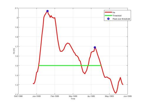
The extreme statistical values of the significant wave height can also be estimated with a different approach to the previous one. The Peaks Over Threshold (POT) approach considers only the maximum value of Hs in a temporal space known as a storm, as can be seen in Figure 2. A storm is defined as an uninterrupted sequence of Hs values that exceed a certain value. This value should be fairly high (threshold), preceded and followed by a lower value. The value chosen for this threshold is highly dependent on local conditions [19].
The POT peak-over-threshold method allows for better selection of extreme events from a data series. This threshold value or also known as storm value, is an empirical data from which an event can be considered as extreme [20]. However, the complexity of this method resides in the threshold selection, since a very low value would ignore the basic conditions of the model [21]. On the other hand, the higher this value is, the less amount of data, therefore, reliability in the fit would be lost.
Figure 2. Example of a storm between two successive crossings of the wave height through a threshold level, Threshold=1.5 m
Figure 3. Example of a deletion of an event whose duration is less than 24 hours, Threshold=5m
It is important also to mention that there are no unified criteria to strictly define what is considered a peak event or extreme event [22]. The fundamental characteristic present in this method is to achieve a population of high and statistically independent values [19].
One way to guarantee this statistical condition is to select a value within the time variable, whose duration must be determined by the characteristics of the environmental phenomenon. In the case of waves, a recommended value is 48 hours. This event duration value is justified since it is the average time that atmospheric disturbances causing waves usually last [21, 23, 24]. In this way, each selected maximum value will belong to different disturbances. In this analysis, a separation of 24 hours will be used, selecting the highest value in said interval, see Figure 3 (first peak).
The distribution of the maximum value in a sequence that occurs above a threshold fits the generalized Pareto distribution [3, 22, 25]. This POT approach has two important advantages over the initial distribution approach discussed above: (a) Select only high values in the significant wave height. The elimination of minor events tends to concentrate the analysis on the regime that dominates the extremes; and (b) storms are statistically independent events, which provide a more solid theoretical foundation and simplify the interpretation of the analysis results (for example, the estimation of the sampling errors involved) [26].
2.1.3 Annual maximum method
The third approach used is the annual maximum or also known as a block-based model. This model considers a population of random values (its distribution is called the parental distribution) from which a set of samples is drawn arbitrarily. Extreme value theory states that, under general conditions, the set’s maximum distribution is a generalized extreme value (GEV) distribution [3, 22]. To use these theoretical bases in a wave analysis, the original population is considered and from this, the maximum significant wave height value that occurs in a period of time, generally one year, is selected. The most relevant data from the sample set is then the maximum height in each year of the multi-year series. A time series of N years therefore gives N values of significant wave height as can be seen in Figure 3. The parameters of this GEV distribution can be estimated from the observed values of Hs [27].
One of the disadvantages present in this method is the importance of having a sufficiently long series of data, not less than 15 years [24], with this a sufficient number of extremes will be obtained to guarantee the adjustment. In cases where the series are very short, it is advisable to do it in blocks of less than one year, taking into account that it can be carried out up to quarterly or monthly maximums, in this case the statistical independence of the events must be guaranteed. In the present case, the series consists of 42 years, so this limitation does not affect the analysis.
The data used are obtained from the spectral separation of variables mentioned above, from which 54056 significant wave height data are obtained, separated in time space by an interval of 6 hours. Each separate series is designated as: Sw1, Sw2, Sw3, Sw4, and Total, the last being the original series, these data are grouped in a matrix (in MATLAB) for statistical analysis. The initial data corresponds to January 1, 1979, at 00:00 and the final data to December 31, 2018, at 18:00.
3.1 Statistical analysis by the initial distribution method
Initially, data lower than a value known as calm sea Hsi (relatively low value of significant wave height) [28] This value will depend on each one of the series, and the values of Hs<Hsi, will be erased [3]. In the case of the processed series, these values are: Sw1, Hsi=0,7 m; Sw2, Hsi=0,1 m; Sw3, Hsi=0,1 m; Sw4, Hsi=0,2 m; and for the Total series, Hsi=1 m.
3.1.1 Histogram adjustment - initial distribution method
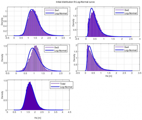
As can be seen in Figure 4 for the partitioned series Sw1, the fit is very good graphically, it has a normal tail, while for the series Sw2 it is a much heavier tail. The Sw3 series presents problems with the fit since it has a large number of central values with few maximums, unlike the Sw4 series which has a heavier tail than the other distributions, it has few minimum values. In general, the total series is very similar to the Sw1 series.
Figure 4. Histograms by the initial distribution method, fit to a Log-Normal curve
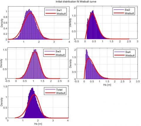
Figure 5. Histograms by the initial distribution method, fit to a Weibull curve
|
|
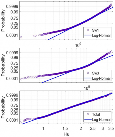
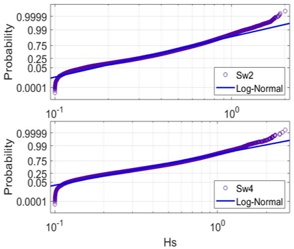
Figure 6. Cumulative probability by the initial distribution method, fit to a Log-Normal curve
|
|
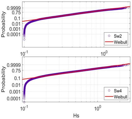
Figure 7. Cumulative probability by the initial distribution method, fit to a Weibull curve
As observed in Figure 5 for the partitioned series Sw1, the fit is poor compared to the previous distribution, the Weibull curve has a fit with more central values, leaving a light tail. Sw2 series is similar to the Log-Normal distribution. Unlike Sw3 series, which presents a better fit to the Weibull distribution. However, the Sw4 series has a heavy tail which fits well this distribution. Finally, the total series presents a poor fit.
With the histogram method, it can be observed that this data series shows a better fit to a Log-Normal distribution, which will be contrasted with the cumulative probability graphs that are presented below.
3.1.2 Adjustment by cumulative probability - initial distribution method
As can be seen in Figures 6 and 7, for all the partitions, especially for Sw3, the adjustment occurs more for average values, which causes a distortion in the adjustment of extreme values.
In relation to the histograms presented above for this method, the following results are presented: The series Sw1, Sw2, and Total behave better in a Log-Normal fit, both in histograms and in cumulative probability. While Sw3 and Sw4 fit better to a Weibull distribution, this is mainly since the low values predominate in these series and not the maximum ones.
From this method, as can be seen in Figures 8 and 9, it is concluded that the total series fit a statistical method, while the partitions do not do so in this way when separating the series by their origin, statistically they behave differently.
3.1.3 Return period - initial distribution method
The return periods are calculated with the occurrence probabilities of each event up to a value of 100 years [29].
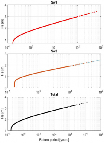
Figure 8. Return period by the initial distribution method, fit to a Log-Normal curve
Figure 9. Return period by the initial distribution method, fit a Weibull curve
Figure 10. Significant wave height as a return period function for the initial distribution method using Log-Normal and Weibull adjustment
Table 1. Return times initial distribution method
|
Return Time [Years] |
Significant Wave Height [m] |
|||||||||
|
Log-N Sw1 |
Log-N Sw2 |
Log-N Sw3 |
Log-N Sw4 |
Log-N Total |
Wb Sw1 |
Wb Sw2 |
Wb Sw3 |
Wb Sw4 |
Wb Total |
|
|
10 |
2.41 |
1.33 |
1.92 |
1.46 |
2.43 |
2.24 |
1.07 |
1.61 |
1.31 |
2.36 |
|
20 |
2.59 |
1.54 |
2.08 |
1.68 |
2.55 |
2.33 |
1.15 |
1.67 |
1.42 |
2.43 |
|
30 |
2.69 |
1.67 |
2.17 |
1.80 |
2.62 |
2.38 |
1.20 |
1.70 |
1.48 |
2.47 |
|
40 |
2.76 |
1.76 |
2.24 |
1.90 |
2.66 |
2.41 |
1.23 |
1.72 |
1.52 |
2.49 |
|
50 |
2.81 |
1.83 |
2.29 |
1.97 |
2.70 |
2.43 |
1.25 |
1.74 |
1.55 |
2.51 |
|
60 |
2.86 |
1.90 |
2.33 |
2.03 |
2.73 |
2.45 |
1.27 |
1.75 |
1.57 |
2.53 |
|
70 |
2.90 |
1.95 |
2.37 |
2.09 |
2.75 |
2.47 |
1.28 |
1.76 |
1.59 |
2.54 |
|
80 |
2.93 |
1.99 |
2.40 |
2.13 |
2.77 |
2.48 |
1.30 |
1.77 |
1.61 |
2.55 |
|
90 |
2.96 |
2.03 |
2.43 |
2.17 |
2.79 |
2.49 |
1.31 |
1.78 |
1.63 |
2.56 |
|
100 |
2.98 |
2.07 |
2.45 |
2.21 |
2.81 |
2.50 |
1.32 |
1.79 |
1.64 |
2.56 |
The return periods for the series: Sw1, Sw2, Sw4 do not present a good fit for extreme values, minor events are very relevant; while in the Sw3 and Total series there is a decrease for low values, which causes a curvature at the beginning of the graph.
As can be seen in Figure 10 and Table 1, for the initial distribution method, there are different return times with both methodologies used. Since there is a statistical analysis, the result differs from the methods used, defining that the greater the return time, the greater the difference, which would cause an overestimation if the appropriate method were not used.
The trend is maintained with the partitioned series and the Total.
3.2 Statistical analysis by the POT peak over threshold method
To carry out the data statistical analysis, it is necessary to define the threshold, for which there are several recommended methods. The reference value in most data is identified as a non-stationary sequence of states in which Hs exceeds the value of 1.5 times the mean annual wave height, that is HsUmbral=1,5¯Hs [30, 31]. With this value we proceed to eliminate lower data and select each storm event from the maximum events. In addition, to guarantee the statistical independence of events, it is necessary to take only values that are distant in temporal space by a period of 24 hours.
3.2.1 Histogram fit - POT method
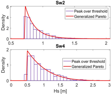
When the data is reduced by a threshold fit, the series must belong to a statistical family known as the generalized Pareto distribution. Then, the data is ordered by histograms and fitted to the statistical distributions, as shown in Figure 11, for the Generalized Pareto Distribution.
As can be seen in Figure 11, the Sw1 series has a heavy tail with very extreme data, while the Sw2 series tail is lighter. The Sw3 series features a normal tail just like the Sw4. Finally, the Total series has a light tail considering their respective aforementioned threshold values.
|
|
Figure 11. Histograms by the peak over threshold method, fit to a Generalized Pareto curve
As can be seen in Figure 12, for the Sw1, Sw4 and Total series: the selected threshold guarantees having enough data and is aligned with the extremes, so it has a good fit. This occurs to a lesser extent with the Sw2 and Sw3 series in which there are extreme values that deviate from the adjustment curve. Compared to the histograms presented above for this method, the following results are shown: The Sw1, Sw4, and Total series behave better in the cumulative probability plots, while the Sw2 and Sw3 series do not, concluding that the heavier the tail, the better it fits this threshold method.
|
|
Figure 12. Histograms by the peak over threshold method, fit to a Generalized Pareto curve
3.2.2 Return period - POT method
As can be seen in Figures 13-15, the return periods are calculated with the probabilities of occurrence of each of the events up to a value of 100 years. As stated earlier in section 1, there are two ways to assess the return period in this method. The first is to find a correction value based on the number of years and the number of events that exceed the said threshold. and another with the average duration time of the storm, that is, the average duration time of the value Hsthreshold.
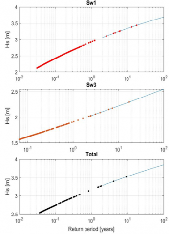
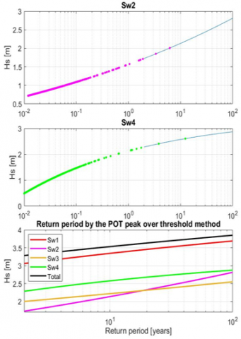
Figure 13. Return period by the POT peak over threshold method, fit to a Generalized Pareto curve
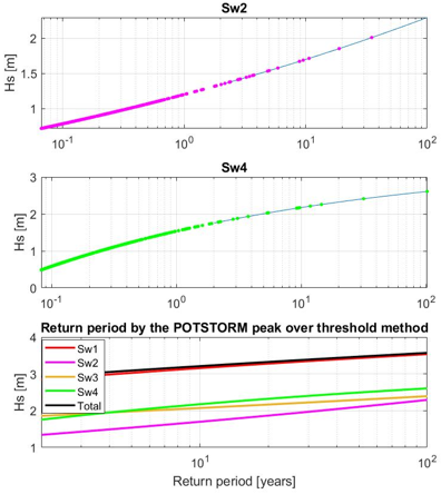
Figure 14. Return period by the POTSTORM peak over threshold method, fit to a Generalized Pareto curve
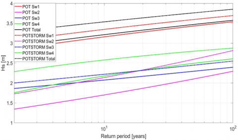
Figure 15. Significant wave height as a function of return time for the peak over threshold method using the number of events and storm duration method
For the first case the results are as follows:
As can be seen in Table 2, the return periods for the series: Sw1, Sw2, Sw3 and Total, present a good adjustment with little relevance of minor events, while in the Sw4 series there is an influence of the low values that cause a curvature at the beginning of the graph. There is a dominance in the Sw1 series over the Total in the return periods, but it does not exceed its value.
Table 2. Return times, peak over threshold method
|
Return Time [Years] |
Significant Wave Height [m] |
|||||||||
|
POT Sw1 |
POT Sw2 |
POT Sw3 |
POT Sw4 |
POT Total |
POTSTORM Sw1 |
POTSTORM Sw2 |
POTSTORM Sw3 |
POTSTORM Sw4 |
POTSTORM Total |
|
|
10 |
3.16 |
1.70 |
2.07 |
2.18 |
3.21 |
3.34 |
2.13 |
2.22 |
2.57 |
3.53 |
|
20 |
3.28 |
1.87 |
2.17 |
2.32 |
3.32 |
3.46 |
2.33 |
2.31 |
2.68 |
3.63 |
|
30 |
3.35 |
1.97 |
2.22 |
2.40 |
3.39 |
3.52 |
2.44 |
2.37 |
2.73 |
3.69 |
|
40 |
3.39 |
2.04 |
2.26 |
2.45 |
3.43 |
3.56 |
2.53 |
2.41 |
2.77 |
3.73 |
|
50 |
3.43 |
2.10 |
2.29 |
2.49 |
3.47 |
3.59 |
2.60 |
2.45 |
2.80 |
3.76 |
|
60 |
3.46 |
2.15 |
2.32 |
2.52 |
3.50 |
3.62 |
2.65 |
2.47 |
2.82 |
3.78 |
|
70 |
3.48 |
2.19 |
2.34 |
2.55 |
3.52 |
3.64 |
2.70 |
2.50 |
2.83 |
3.80 |
|
80 |
3.50 |
2.23 |
2.36 |
2.57 |
3.54 |
3.66 |
2.74 |
2.51 |
2.85 |
3.82 |
|
90 |
3.52 |
2.26 |
2.38 |
2.59 |
3.56 |
3.68 |
2.78 |
2.53 |
2.86 |
3.84 |
|
100 |
3.54 |
2.29 |
2.39 |
2.60 |
3.57 |
3.69 |
2.81 |
2.55 |
2.87 |
3.85 |
3.3 Statistical analysis by the method of annual maximums
For the following method it is necessary to examine the data and determine the high values for each year since we are essentially working with maximums. However, by choosing only the highest value of a data set, it is possible to ignore extreme events that occurred in that time period that may be similar to or even greater than the maximum values of other intervals. For this series it is essential to analyze their behavior.
In addition, separation by blocks can be arbitrary, since if there is not enough data, it is necessary to group them on a quarterly, monthly, or daily basis, losing reliability in the model. In the case of waves, the highest values that fit a Generalized extreme value distribution (GEV) are selected. The selected data is presented below:
3.3.1 Adjustment by histograms - method of annual maximums
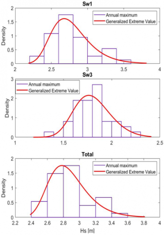
As can be seen in Figure 16, in the annual maximum’s method, there are 42 years and a maximum in each of these blocks, complying with the recommendations in the reference [24], who advises having a minimum of 15 data.
|
|
Figure 16. Histograms by the method of annual maximums method, fit to a GEV curve
3.3.2 Adjustment by cumulative probability - method of annual maximums
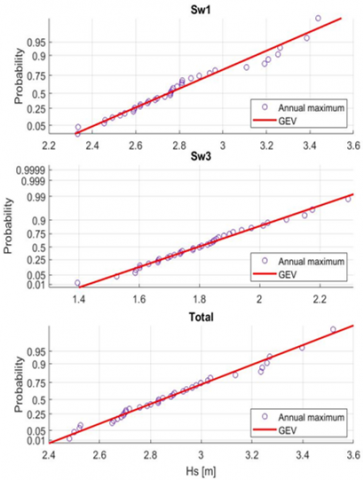
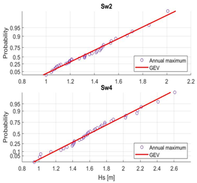
As can be seen in Figure 17, the Sw1 series presents a slight deviation from the fit line at its maximum values. This is because it has several core values that dominate the data. While for the Sw2, Sw3, Sw4, and Total series, it can be seen that the fit to the maximum values is higher and has better confidence in the expected results.
In the annual maximum’s method, there are 42 years and a maximum in each of these blocks, complying with the recommendations in the reference [24], who advises having a minimum of 15 data.
|
|
Figure 17. Cumulative probability by the method of annual maximums, fit to a GEV curve
3.3.3 Return period - annual maximum method
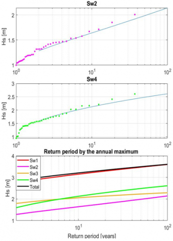
As can be seen in Figure 18, there is a complete domination of the Sw1 series in the return periods, but in this case its value is not exceeded, so only by analyzing the total series can an adequate value of the return period be obtained (Table 3).
Table 3. Return times method of annual maximums
|
Return Time [Years] |
Significant Wave Height [m] |
||||
|
Sw1 |
Sw2 |
Sw3 |
Sw4 |
Total |
|
|
10 |
3.15 |
1.64 |
2.06 |
2.13 |
3.21 |
|
20 |
3.29 |
1.79 |
2.14 |
2.29 |
3.34 |
|
30 |
3.37 |
1.88 |
2.18 |
2.38 |
3.41 |
|
40 |
3.43 |
1.94 |
2.21 |
2.44 |
3.46 |
|
50 |
3.47 |
1.99 |
2.23 |
2.49 |
3.50 |
|
60 |
3.51 |
2.03 |
2.25 |
2.52 |
3.53 |
|
70 |
3.53 |
2.06 |
2.26 |
2.55 |
3.55 |
|
80 |
3.56 |
2.09 |
2.27 |
2.57 |
3.57 |
|
90 |
3.58 |
2.12 |
2.28 |
2.60 |
3.59 |
Figure 18. Return period by the annual maximum’s method, fit a GEV curve
There is a complete domination of the Sw1 series in the return periods, but in this case its value is not exceeded, so only by analyzing the total series can an adequate value of the return period be obtained.
3.4 Comparing results
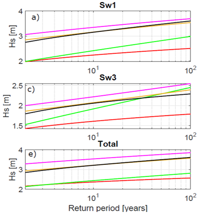
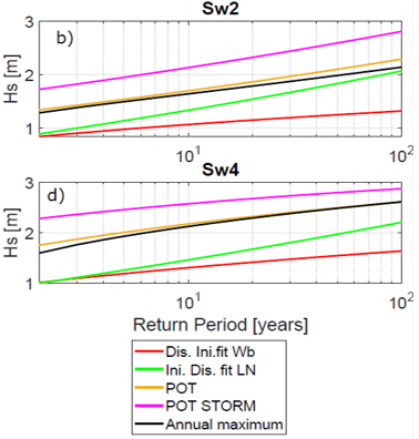
This is verified by means of a statistical T-student test for two samples assuming unequal variances by which the null hypothesis is accepted or rejected for the different cases shown in Figure 19.
It can be deduced from Figure 19(a) that there is a relationship between the annual maximum method and the peak over threshold method using the amount of events technique. On the other hand, with the peak over threshold method using the average storm duration technique, a higher value of significant wave height is obtained. While the initial distribution methods have very low values, the latter is the one with the least reliability.
Figure 19(b) shows that there is agreement between the annual maximum method and the peak over threshold method using the amount of events technique. However, there is a greater difference than in the previous case, while with the peak over threshold method and with the average storm duration technique, there is a higher value of significant wave height. On the other hand, with the initial distribution methods, very low values are obtained, except with the Log-Normal adjustment method, which is very close to annual maximums.
|
|
Figure 19. Return period: a) Sw1, b) Sw2, c) Sw3, d) Sw4, e) Total
Additionally, in the Figure 19(c) can be observed that, as in the previous cases, the similarity between the annual maximum methods is maintained with the peak over threshold method using the amount of events technique. In contrast, the peak over threshold method with the average storm duration technique has a higher value of significant wave height, but in this case, higher values are reached with the Log-Normal adjustment initial distribution method. Figure 19(d) shows that the trends remain the same as in the Sw1 series. Figure 19(e) shows a relationship between the annual maximum method with the peak over threshold method using the amount of events technique. While the peak over threshold method with the average storm duration technique has a higher value of significant wave height. On the other hand, with the initial distribution methods, there are very low values, the latter with the least reliability, and therefore related to the dominant series Sw1.
In previous studies [32], it has been determined that four wave systems can be identified for the analyzed place. The EVA methods were applied to the total wave series, and to the partial time series of each of these systems. In the analysis (in all cases) it is observed that the partial series WS1 is dominant at the extremes, and therefore its distribution resembles the distribution of the total series. The other series WS2, WS3, WS4 result in extreme values for significantly shorter return periods of 100 years. As observed in Figure 19, for the 5 methods, the Sw1 series (red line) is related to the Total series (black line). This was verified by means of a goodness-of-fit test with a similarity index of 90%.
For the peak over threshold method, there are two techniques for calculating the return period. The first uses a correction factor based on the number of events that crosses the threshold (POT) and the second uses the duration of the average storm (POTSTORM). As can be seen in Figure 19, with POTSTORM (magenta line) higher values of the variable are obtained for return periods of 100 years compared to POT (blue line). In addition, the latter presents more consistent values with the annual maximum’s method (black line).
Two methods (POT and AM) yield the same results, in statistically terms. When evaluating return periods using the peak over threshold and annual maximum methods, very similar results are obtained. This is verified with a t-student test with an index of 0.05, approving the null hypothesis, as shown in Table 4.
Table 4. Return times up to 100 years for the peak over threshold and annual maximum methods
|
Return Time [Years] |
Hs [m] |
|||||||||
|
Sw1 |
Sw2 |
Sw3 |
Sw4 |
Total |
||||||
|
POT |
AM |
POT |
AM |
POT |
AM |
POT |
AM |
POT |
AM |
|
|
50 |
3.43 |
3.47 |
2.10 |
1.99 |
2.29 |
2.23 |
2,49 |
2.49 |
3.47 |
3.50 |
|
60 |
3.46 |
3.51 |
2.15 |
2.03 |
2.32 |
2.25 |
2,52 |
2.52 |
3.50 |
3.53 |
|
70 |
3.48 |
3.53 |
2.19 |
2.06 |
2.34 |
2.26 |
2,55 |
2.55 |
3.52 |
3.55 |
|
80 |
3.50 |
3.56 |
2.23 |
2.09 |
2.36 |
2.27 |
2,57 |
2.57 |
3.54 |
3.57 |
|
90 |
3.52 |
3.58 |
2.26 |
2.12 |
2.38 |
2.28 |
2,59 |
2.60 |
3.56 |
3.59 |
|
100 |
3.54 |
3.60 |
2.29 |
2.14 |
2.39 |
2.29 |
2,60 |
2.61 |
3.57 |
3.61 |
|
Hypothesis testing t-test α=0.05 |
t-statistic |
0.67 |
t-statistic |
1.45 |
t-statistic |
1.62 |
t-statistic |
0.16 |
t-statistic |
0.46 |
|
P(T<=t) two tails |
0.51 |
P(T<=t) two tails |
0.16 |
P(T<=t) two tails |
0.12 |
P(T<=t) two tails |
0.88 |
P(T<=t) two tails |
0.65 |
|
|
Critical t-value (two tailed) |
2.10 |
Critical t-value (two tailed) |
2.10 |
Critical t-value (two tailed) |
2,10 |
Critical t-value (two tailed) |
2.10 |
Critical t-value (two tailed) |
2.10 |
|
|
As 0.67<2.10 Null Hypothesis Accepted |
As 1.45<2.10 Null Hypothesis Accepted |
As 1.62<2.10 Null Hypothesis Accepted |
As 0.16<2.10 Null Hypothesis Accepted |
As 0.46<2.10 Null Hypothesis Accepted |
||||||
Notes: Data Separation indicates the presence of different populations with different characteristics. To guarantee data independence, it is convenient to separate them whenever possible.
The primary objective of this research endeavor is to employ various extreme value analysis (EVA) techniques in the analysis of wave time series data. A notable innovation in this context is the application of EVA methods to wave data, wherein the principal variable of interest, the wave spectrum, facilitates the identification and separation of distinct events based on their origins. Consequently, this approach enables a more rigorous adherence to the essential statistical prerequisites for EVA, particularly the requirement of event independence, both in physical and statistical terms.
Three distinct EVA methodologies have been utilized in this study, namely the Initial distribution method, the peak over threshold method, and the annual maximum value method. The Initial distribution method predominantly serves a descriptive function, while the latter two methods are predictive in nature, enabling the projection of extreme values over time periods that extend beyond the length of the data series. It is worth noting that EVA methods are conventionally employed in engineering studies for the determination of design values. However, in the present study, their application has been instrumental in the development of algorithms aimed at consolidating this knowledge and applying it in novel geographical locations.
The main parameter sought by applying EVA is the value of a variable associated with a specific return period, with particular attention to the 100-year return period in this context. The significant wave height Hs, for a return period of 100 years, is used as a design value in most marine structures, such as coastal zone protections.
In the context of selecting an appropriate threshold value, it is imperative to opt for values that ensure both statistical and physical independence of events, avoiding extremes that are either too high or too low. In accordance with Boccotti’s research [30], a threshold value of 1.5 times the significant wave height (Hs) has been chosen as the threshold value, although it is acknowledged that further investigation into the suitability of this value is warranted.
Among the various EVA methods considered, the peak over threshold method, in conjunction with the technique of counting events above the threshold, has been found to be particularly suitable. Conversely, the use of the annual maximum technique in conjunction with the peak over threshold method, along with the introduction of the storm duration parameter, has been found to result in more complex calculations and an overestimation of values. Accordingly, it is not advisable to employ the initial distribution method as a projection method in the context of EVA.
Selecting the appropriate threshold value is a meticulous and analytical process, contingent upon the unique characteristics of the dataset and the underlying physical phenomenon. Opting for a low threshold value may include non-extreme events, while high threshold values pose the risk of working with an insufficient number of data points, compromising the reliability of the model. In this study, the threshold value has been set at 1.5 times the average annual wave height [30, 31] as a pragmatic choice.
Through this study, it is evident that the peak over threshold method, when coupled with event-counting techniques, exhibits similarities with the annual maximum method. Moreover, the algorithm for calculating the return period is considerably simpler in the former approach.
[1] Méndez, F.J., Menéndez, M., Luceño, A., Losada, I.J. (2007). Analyzing monthly extreme sea levels with a time-dependent GEV model. Journal of Atmospheric and Oceanic Technology, 24(5): 894-911. https://doi.org/10.1175/JTECH2009.1
[2] Young, I.R., Vinoth, J., Zieger, S., Babanin, A.V. (2012). Investigation of trends in extreme value wave height and wind speed. Journal of Geophysical Research: Oceans, 117(C11): 1-13. https://doi.org/10.1029/2011JC007753
[3] Holthuijsen, L.H. (2010). Waves in Oceanic and Coastal Waters. Cambridge University Press.
[4] Caires, S., Groeneweg, J., Sterl, A. (2009). Past and future changes in the North Sea extreme waves. In Coastal Engineering 2008: (In 5 Volumes), pp. 547-559. https://doi.org/10.1142/9789814277426_0046
[5] Sterl, A., Caires, S. (2005). Climatology, variability and extrema of ocean waves: The Web-based KNMI/ERA-40 wave atlas. International Journal of Climatology: A Journal of the Royal Meteorological Society, 25(7): 963-977. https://doi.org/10.1002/joc.1175
[6] Jácome, E. (2022). Análisis de Condiciones Extremas de Oleaje en el Archipiélago de Galápagos. Revista Politécnica, 50(1): 7-14.
[7] Dee, D.P., Uppala, S.M., Simmons, A.J., Berrisford, P., Poli, P., Kobayashi, S., Vitart, F. (2011). The ERA-Interim reanalysis: Configuration and performance of the data assimilation system. Quarterly Journal of the Royal Meteorological Society, 137(656): 553-597. https://doi.org/10.1002/qj.828
[8] Portilla-Yandún, J., Cavaleri, L., Van Vledder, G.P. (2015). Wave spectra partitioning and long term statistical distribution. Ocean Modelling, 96: 148-160. https://doi.org/10.1016/j.ocemod.2015.06.008
[9] Portilla, J., Ocampo-Torres, F.J., Monbaliu, J. (2009). Spectral partitioning and identification of wind sea and swell. Journal of Atmospheric and Oceanic Technology, 26(1): 107-122. https://doi.org/10.1175/2008JTECHO609.1
[10] Portilla, J., Caicedo, A.L., Padilla-Hernández, R., Cavaleri, L. (2015). Spectral wave conditions in the Colombian Pacific Ocean. Ocean Modelling, 92: 149-168. https://doi.org/10.1016/j.ocemod.2015.06.005
[11] Portilla-Yandún, J., Salazar, A., Cavaleri, L. (2016). Climate patterns derived from ocean wave spectra. Geophysical Research Letters, 43(22): 11-736. https://doi.org/10.1002/2016GL071419
[12] Portilla-Yandún, J. (2018). Open access atlas of global spectral wave conditions based on partitioning. In International Conference on Offshore Mechanics and Arctic Engineering, 51333: V11BT12A051. https://doi.org/10.1115/OMAE2018-77230
[13] Mitchell, T.P., Wallace, J.M. (1992). The annual cycle in equatorial convection and sea surface temperature. Journal of Climate, 5(10): 1140-1156. https://doi.org/10.1175/1520-0442(1992)005%3C1140:TACIEC%3E2.0.CO;2
[14] Chelton, D.B., Freilich, M.H., Esbensen, S.K. (2000). Satellite observations of the wind jets off the Pacific coast of Central America. Part II: Regional relationships and dynamical considerations. Monthly Weather Review, 128(7): 2019-2043. https://doi.org/10.1175/1520-0493(2000)128%3C2019:SOOTWJ%3E2.0.CO;2
[15] MacAfee, A.W., Wong, S.W. (2007). Extreme value analysis of tropical cyclone trapped-fetch waves. Journal of Applied Meteorology and Climatology, 46(10): 1501-1522. https://doi.org/10.1175/JAM2555.1
[16] Fisher, R.A.,Tippett, L.H.C. (1928). Limiting forms of the frequency distribution of the largest or smallest member of a sample. In Mathematical Proceedings of the Cambridge Philosophical Society, 24(2): 180-190. https://doi.org/10.1017/S0305004100015681
[17] Goda, Y. (1992). Uncertainty of design parameters from viewpoint of extreme statistics. Journal of offshore Mechanics and Arctic Engineering, 114(2): 76-82. https://doi.org/10.1115/1.2919962
[18] Ewans, K., Jonathan, P. (2008). The effect of directionality on Northern North Sea extreme wave design criteria. Journal of offshore Mechanics and Arctic Engineering, 130(4): 041604. https://doi.org/10.1115/1.2960859
[19] Portilla-Yandún, J., Jácome, E. (2020). Covariate extreme value analysis using wave spectral partitioning. Journal of Atmospheric and Oceanic Technology, 37(5): 873-888. https://doi.org/10.1175/JTECH-D-19-0198.1
[20] Ferreira, J.A., Soares, C.G. (1998). An application of the peaks over threshold method to predict extremes of significant wave height. Journal of Offshore Mechanics and Arctic Engineering, 120(3): 165-176. https://doi.org/10.1115/1.2829537
[21] Simiu, E., Heckert, N.A. (1996). Extreme wind distribution tails: A “peaks over threshold” approach. Journal of Structural Engineering, 122(5): 539-547. https://doi.org/10.1061/(ASCE)0733-9445(1996)122:5(539)
[22] Coles, S., Bawa, J., Trenner, L., Dorazio, P. (2001). An Introduction to Statistical Modeling of Extreme Values. London: Springer. https://doi.org/10.1007/978-1-4471-3675-0
[23] Walton, T.L. (2000). Distributions for storm surge extremes. Ocean Engineering, 27(12): 1279-1293. https://doi.org/10.1016/S0029-8018(99)00052-9
[24] Herrera, F.J.G. (2013). Modelización estadística de eventos extremos de oleaje y nivel del mar. Statistical analysis of waves and sea level extreme values. http://hdl.handle.net/10553/11243.
[25] Castillo, E. (1988). Extreme Value Theory in Engineering. Elsevier. https://doi.org/10.1016/C2009-0-22169-6
[26] Campos, R.M., Alves, J.H.G.M., Soares, C.G., Guimaraes, L.G., Parente, C.E. (2018). Extreme wind-wave modeling and analysis in the south Atlantic Ocean. Ocean Modelling, 124: 75-93. https://doi.org/10.1016/j.ocemod.2018.02.002
[27] Caires, S. (2009). A comparative simulation study of the annual maxima and the peaks-over-threshold methods. Deltares report 1200264-002 for Rijkswaterstaat, Waterdienst.
[28] Gumbel, E.J. (1958). Statistics of Extremes. Columbia University Press. https://doi.org/10.7312/gumb92958
[29] Carter, D.J.T., Challenor, P.G. (1981). Estimating return values of environmental parameters. Quarterly Journal of the Royal Meteorological Society, 107(451): 259-266. https://doi.org/10.1002/qj.49710745116
[30] Boccotti, P. (2000). Wave Mechanics for Ocean Engineering. Elsevier.
[31] Fedele, F., Arena, F. (2010). Long-term statistics and extreme waves of sea storms. Journal of Physical Oceanography, 40(5): 1106-1117. https://doi.org/10.1175/2009JPO4335.1
[32] Portilla-Yandún, J. (2018). The global signature of ocean wave spectra. Geophysical Research Letters, 45(1): 267-276. https://doi.org/10.1002/2017GL076431