Phaiboon Boupha![]() | Ponthep Vengsungnle
| Ponthep Vengsungnle![]() | Aphichat Srichat
| Aphichat Srichat![]() | Chaiyan Junsiri
| Chaiyan Junsiri![]() | Kittipong Laloon
| Kittipong Laloon![]() | Sakkarin Wangkahart
| Sakkarin Wangkahart![]() | Kaweepong Hongtong
| Kaweepong Hongtong![]() | Sahassawas Poojeera*
| Sahassawas Poojeera*![]()
© 2024 The authors. This article is published by IIETA and is licensed under the CC BY 4.0 license (http://creativecommons.org/licenses/by/4.0/).
OPEN ACCESS
This article concerned the mixing of high-viscosity fluids using close-clearance impellers in a cylindrical tank (caustic soda and water). This investigation employed a numerical model to evaluate the performance of three distinct impeller designs at rotational speeds of 10, 20, and 30 rpm. The analysis concentrated on parameters indicative of mixing efficiency, including color dispersion, vector movement of the mixed material, temperature gradients from the tank wall to the center, and the average temperature within the agitator tank. Results indicated that the ribbon impeller operating at 30 rpm achieved the highest average temperature (53.69℃) across all measurement points within the mixing vessel compared to the other impeller configurations. This finding suggests that the ribbon impeller design is most effective in promoting optimal mixing. Additionally, the heat distribution within the tank exhibited a high degree of uniformity, which contributed to consistent vector movement of the mixed material. Furthermore, the temperature gradient, representing the average temperature variation from the tank wall to the center at each depth, was most pronounced with the ribbon impeller design.
mathematical model, temperature distribution, types of blades, agricultural waste, stirrer, forming materials
The increasing environmental concerns regarding the excessive utilization of plastic packaging, which lead to a substantial volume of non-biodegradable waste, have driven the demand for environmentally friendly alternatives [1, 2]. Bioplastics made from biodegradable sources provide a promising solution to the challenges of packaging waste disposal [3]. In Thailand, cornstarch and cassava starch are commonly used as raw materials to produce bioplastic. However, their high production costs have led to the need to explore alternative materials. Natural resources that are abundant in cellulose fibers, such as rice straw, sugarcane bagasse, and banana peels, are considered viable options for producing low-cost, bio-based packaging [4]. The materials need to be processed through drying, size reduction, and pulverization [4]. Next, they are treated with soda ash or sodium hydroxide (NaOH), washed, pulverized, and formed into sheets using paper molds [5-7].
In the soda ash-assisted material breakdown process, the design of the impeller blades and the configuration of the mixing tank play a crucial role. Uneven temperature distribution can lead to hotspot formation, causing localized burning or material degradation. Similarly, colder areas can hinder proper melting and blending, resulting in a weakened product with compromised structural integrity. Non-uniform mixing can also disrupt the shaping process, increasing processing times and energy consumption. In the past, impeller designs were developed using empirical knowledge or trial-and-error methods, which are time-consuming, resource-intensive, and may need to be revised to produce optimal results. In response to these limitations, the present study employed mathematical modelling as a potent instrument for analyzing, predicting, and optimizing impeller configurations [8].
Agitator reactors in the chemical industry are very common, and they are important for both liquid and solid-phase chemicals to obtain products from the chemical reaction between solid-phase and liquid-phase components [9]. Agitation plays an important role in a wide range of industries, such as fine chemicals, agrochemicals, pharmaceuticals, petrochemicals, biotechnology, polymer processing, pulp and paper, color mineral processing, and automotive surfaces [10, 11]. The design of an agitator reactor equipped with impellers should consider relevant parameters such as conservation of mass and momentum, turbulent kinetic energy, energy consumption, agitation time, heat and mass transfer, and mechanical properties of the impellers [12] to monitor the flow field, temperature, and concentration, as well as heat flux and mass flux [13, 14]. The quality of the final chemical product is determined by the solid particles’ remaining in suspension within the liquid phase for as long as possible for the chemical reaction to take place [9]. Many experimental studies on agitation processes have been conducted over the past decades [15, 16]. Advanced experimental optical techniques, especially Particle Image Velocimetry (PIV), are widely used at laboratory scales for hydrodynamic characterization [17, 18]. However, it is not suitable for use in studying industrial agitator reactors. It is mainly used for local spatial description for various reasons, such as equipment size, opaque walls, and media. Computer simulation models are therefore used to study various aspects of agitator reactor design and to predict product formation during chemical reactions [19] or culture processes [20, 21].
To quantify the impact of factors that play an important role in the optimization of agitator reactor design, it is often necessary to use Computational Fluid Dynamics (CFD) numerical models such as geometry, fluid mechanics, as well as heat and mass transport [22, 23]. One of the challenging tasks involving the agitator reactor simulation is simulating the rotation of the reactor [22]. Mechanical agitation or mechanical compounding is commonly used to improve mixing in industrial containers. Inside the agitator reactor, rotating parts are installed to increase the mass transfer rate and homogeneous fluid [24]. The design and selection of the agitator reactor’s rotating parts play an important role in the mixing process [25, 26]. The simulation of an agitator reactor is Fluid-Structure Interaction (FSI) [27]. The simulation of an agitator reactor is Fluid-Structure Interaction (FSI) [27]. Because of the complexity of FSI problems, as a result, developing analytical solutions to these problems is difficult. As a result, numerical simulations are often used to study FSI to solve equations that include fluid motion and deformable materials [28]. Subsequently, different numerical investigations were carried out using FSI analysis on the fluid-solid structure interaction. These results demonstrate that FSI analysis is suitable for studying FSI in agitation equipment [29-31]. According to the literature mentioned above, the behavior of the fluid in an agitator reactor depends on the shape of the impellers. The important reason for the mixing process and flow behavior of the agitator reactor is influenced by geometric parameters, including number of impellers, thickness of impellers, width of impellers, height of impellers, angle of impellers, and the distance between the impeller and the bottom of the stirred tank reactor, for example [12]. Methods have been proposed to establish the relationship between objective functions (such as energy consumption, agitation time, and maximum equivalent stress, for example) and effective parameters (or design parameters) in the mixing process within the agitator reactor [32-34]. Multi-objective optimization (MOO) techniques can optimize the impellers’ geometry and allow the optimal agitator design [35].
Over the past three decades, computational fluid dynamics (CFDs) has proven to be a useful [36-38] and important tool in the chemical industry [12]. Recent studies addressed three issues in improving the accuracy of simulations of agitation inside the agitator reactor using the CFD technique: (1) the use of models for the reasonable turbulence consideration during the mixing process [39, 40]; (2) consideration of suitable models for simulating non-Newtonian fluids [41]; and (3) consideration of suitable boundary conditions for mixing processes [42, 43]. Numerous studies worldwide have performed a numerical analysis of turbulent multi-phase flows specific to agitator reactors with various configurations using CFD for experts and researchers (ANSYS Fluent, ANSYS CFX) [18, 44-47]. Stachnick and Jakubowski performed numerical simulations with Ansys CFX 18.1 using a free surface model of a three-phase Volume of Fluid (VOF) to analyze the movement and formation of solid particles from the separator used in the beer brewing industry. The numerical results were compared with the experimental results, proving that the used model was suitable for the analyzed phenomena and provided accurate and reliable results for the flow and sedimentation [48].
In addition, Tembely et al. [49] used the VOF method to analyze two-phase flow within a porous medium, which considers the dynamic contact angle and hysteresis via Operation and Manipulation (OpenFOAM). The numerical results are compared with the experimental results, and good conclusions are drawn. McCraney et al. [50] presented a numerical method for the symmetric draining of capillary liquids in simple interior corners using Interfoam software (OpenFOAM) and VOF model by comparing numerical results with experimental results. The accuracy of the numerical results is good. He et al. [51] presented the results of using an improved VOF - discrete element method (DEM) model for soil–water interaction studies. Silva and colleagues used OpenFOAM and ANSYS Fluent to study gas and liquid flow at the microscopic level. A study was conducted to evaluate the ability of both software to predict flow fields using different models for multi-phase flow, VOF, and A piecewise linear interface calculation (PLIC) in ANSYS Fluent and MULES/isoAdvector in OpenFOAM. After verifying the obtained results with experimental data, the research concludes that ANSYS Fluent provides more accurate results for this type of flow [52].
Another concern of researchers is selecting the most appropriate model for modeling the suspension volume of the solid inside the liquid from the existing CFD model [53, 54] for learning and improving the complex phenomenon of multi-phase flow. Many researchers used two main methods to demonstrate multi-phase flow behavior in the CFD model of gas and liquid containers: Eulerian-Lagrangian and Eulerian-Eulerian approach [9, 55-57]. The Eulerian-Eulerian approach is a widely used approach for the CFD model of turbulent containers, which is detailed as follows [40]. Modelling multi-phase connections [58, 59] such as drag force [60, 61], lift force [61], and virtual mass force [62], for example. Many models are used in the analysis, for example, using Reynolds-Averaged Navier-Stokes (RANS) for simulating the turbulent flow behaviour, one or two equations using Length eddy simulation (LES) [63, 64] and Direct numerical simulation [65] in the analysis. The average flow and turbulence of the agitator reactor were accurately assessed using the 3D k-ε turbulence model [44]. Another model used for simulating anisotropic turbulent flow in the agitator reactors is the Explicit Algebraic Stress Model (EASM) [66]. In addition, the Scale-Adaptive Simulation turbulence model (SAS) was used to investigate the turbulent flow field occurring in the agitator reactor [67]. There are three pieces of research using three methods for simulating impeller motion: Sliding Mesh (SM), Multiple Frames of Reference (MFR), and Single Rotating Frame (SRF) [68]. For the SM technique, two fluid domains, a rotating domain and a stationary domain, must be defined. The SM technique requires a solution to the non-stationary problem of the flow field [69]. For example, the research of de Lamotte et al. [18] used MRF and SM techniques to simulate the movement of the impellers. The model allows for comparisons between different methods and the identification of important physical phenomena. Two decomposition techniques such as proper orthogonal decomposition (POD) and dynamic mode decomposition (DMD) were then used. Both methods are complementary and emphasize different physical characteristics [70-73]. Considering the results from the most suitable model for the research, the RNG $k-\varepsilon$ turbulence model provides sufficient accuracy within a reasonable computation time, and the Eulerian multi-phase model for calculating liquid-solid mixtures [6] is well-established and has relatively low computational costs [39].
Numerous research studies have extensively focused on various mixing processes, especially the mixing of soda ash (sodium hydroxide, NaOH). These studies investigated the effect of mixing soda ash with different substances, such as gases, liquids, and solids, within impeller mixing tanks [74-76]. Additionally, there are studies on multiphase mixing in stirred tanks involving liquid-solid and gas-liquid phases [77], optimizing mixing for mercaptan removal from kerosene using soda ash and a fixed mixer under varying conditions [5], and analyzing the rapid neutralization reaction between HCl and NaOH when mixing two liquids in a tank [78].
There are many studies on mixing processes involving solids and liquids. However, there are few studies on soda ash mixing in agricultural materials. With the lack of research in this field, a combined modelling and experimental approach are required to determine the optimal impeller design for soda ash mixing in stirred tanks. Selecting an appropriate impeller can substantially decrease processing time and costs and improve the efficiency of material mixing. Consequently, this can result in enhanced fiber dispersion and fiber bonding and greater stability in the fiber arrangement of the final product.
The objective of this study was to find out more detailed information about the effects of different impellers and analysis of caustic soda mixing tanks using computational fluid dynamics) under the three types of impellers, including two-paddle impellers, six-blade impellers, and Helical ribbon impellers, at three speed levels. Computational fluid dynamics modelling was used in the analysis. For this purpose, a multi-phase Eulerian-Eulerian model combined with an RNG $k-\varepsilon$ turbulence model was chosen to simulate a turbulent vessel. The CFD model was first validated by reported experimental data [14, 39]. In addition, the CFD modelling technique was used to study the influence of the impeller patterns to compare the agitator’s temperature distribution and mixing time, speed, energy consumption, and mixing quality.
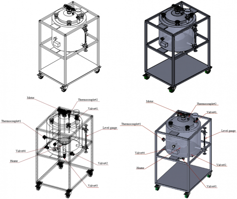
Agitators are produced in various sizes and styles, including marine propellers, foils, axial and radial flow turbines, and anchor-shaped stirrers. The different rotating impeller patterns result in different flow patterns, resulting in the agitator being able to operate in high and low viscosity conditions. However, simple mixing tasks such as mixing liquids with the same viscosity, well-combined liquid within the tank, and liquids that are constantly circulating in the tank for distributing heat from the heat-controlled walls, for example. For difficult agitation cases, including fluids with different viscosities, mechanical agitation of high-viscosity fluids has become a serious concern in all industries today [79]. The dispersion of powder and bonding with water, the making of emulsions or suspensions, and the dissolution or fine grinding of solid raw materials, for example, the agitator took a very long time to complete these mixing processes or may not be able to do it at all. The agitator modeling is shown in Figure 1.
Figure 1. The agitator modelling
2.1 Characteristics of blade impellers
This is a numerical analysis of the impeller behavior under the change of three types of impellers, namely two-paddle impellers, six-blade impellers, and helical ribbon impellers. The ribbon impeller, a type of close-clearance impeller, is characterized by its helical, spring-like metal blades that are enclosed within a stationary mixing tank. These blades are attached to a rotating shaft that can operate at various rotational speeds. Unlike other impeller designs, ribbon impellers typically generate minimal heat during operation due to the reduced shearing action between the material, the blades, and the tank walls at three-speed levels. The three impeller types employed in this study all fall under the category of close-clearance impellers, characterized by their downward-facing blades positioned at the tank bottom. These blades feature gaps between them that allow the material or liquid to flow through during mixing, facilitating material movement within the tank and mitigating heat buildup near the tank walls. CFD was used in the analysis to compare the temperature, flow direction, speed, and time that occur on the agitator and impellers. The use of a mechanical agitator with a suitable impeller will result in uniform agitation of the liquid [80]. Reports show that after optimizing the impeller shape, the circulating flow rate generated by the impeller was greatly increased, resulting in a significant reduction in agitation time, and the demand for electrical energy decreased [81]. The analysis was of the agitation tank used to mix water with caustic soda with three types of impellers, as shown in Figures 2 to 4.
Figure 2. Characteristics of two-paddle impellers
Figure 3. Characteristics of six-blade impellers
Figure 4. Characteristics of Helical ribbon impellers
Previous studies of impellers have various characteristics; each characteristic has different advantages and disadvantages. The perforated impeller in Figure 2 is a two-paddle impeller installed at the end of the shaft with a threaded screw for fixing the shaft. A two-paddle impeller is always sufficient for mixing high-viscosity liquids [79]. Two impellers were placed opposite each other at an angle of 45 degrees, alternating sides on both sides. Many studies reported that placing the impellers at 30 degrees is the most appropriate angle for the two-paddle impeller [82]. The reports stated that the axial flow style agitator is generally considered the most suitable agitator. The six-blade impeller in Figure 3 is one of the most widely used axial flow impellers. In the present study [83], a ribbon bar impeller shown in Figure 4, a batch tank reactor equipped with a Helical ribbon impeller, was designed and manufactured. Using this reactor significantly increases production efficiency and shortens the required residence time [84] to create an axially symmetrical circulation cell that moves liquid down the edge of the tank and up near the center of the tank [85]. The tank has a diameter of 400 mm, a total height of 410 mm, a cylindrical section height of 250 mm, a cone section height of 160 mm, a tank bottom diameter of 50 mm, and the impeller was installed at a depth of 130 mm from the edge of the tank.
2.2 Mixture properties
This simulation analysis simulates chemical pretreatment to remove the starch and increase the percentage of material fibers by using sodium hydroxide (caustic soda) at a concentration of 7% and boiling for 1 hour. Then, the material is rinsed with water to remove sodium hydroxide from the material. The analysis analyzed the mixing between two types of mixtures, namely water and sodium hydroxide (caustic soda), in a ratio of 9:1 to study the agitation results of various types of tanks and impellers to see how they differ in efficiency and which type is more appropriate.
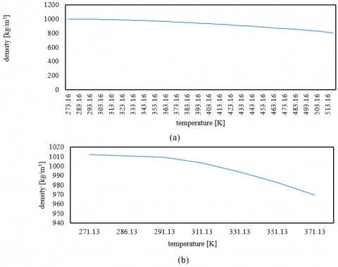
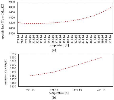
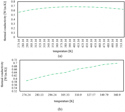
Preliminary analysis of both mixtures was performed by gradually increasing the mixtures’ temperature to check and understand the important properties by considering the trend results before analyzing the mixture in the agitator and various impellers. The properties of the mixture used in the preliminary analysis are density (density[kg/m3], dynamic viscosity [Pa*s]), specific heat ([Cp or J/(kg.K)], and thermal conductivity [W/(m.K)]), as shown in Figures 3 and 5-8.
Figure 5. (a) water temperature versus density; (b) caustic soda temperature versus density
Figure 6. (a) water temperature versus dynamic viscosity; (b) caustic soda temperature versus dynamic viscosity
Figure 7. (a) water temperature versus specific heat; (b) caustic soda temperature versus specific heat
Figure 8. (a) water temperature versus thermal conductivity; (b) caustic soda temperature versus thermal conductivity
The more the mixture’s viscosity can be reduced, the more effective the mixing will be. From Figure 5, the viscosity decreases even more as the temperature increases. For ordinary water, shown in Figure 5(a), the viscosity at high and low temperatures is almost no difference. As shown in Figure 5(b), the viscosity gradually decreases with the given temperature if it is caustic soda. This is consistent with impeller tests, which found that viscosity increases as fluid moves away from the impeller. The suction flow reaches a high viscosity where the low-pressure zone created behind the impeller accelerates the deformation rate and causes the viscosity to decrease again [41].
2.3 Defining the model used in the analysis
The analysis employed in this study utilizes a steady-state approach, a methodology that examines fluid flow under the assumption that the system's conditions remain constant over time [86, 87]. This implies that parameters such as flow velocity, applied forces, and temperature do not exhibit temporal variations or experience only minimal changes. The gravitational force of the Earth, which induces convective heat transfer, is incorporated into the analysis. Computational fluid dynamics (CFD) studies, as evidenced in numerous investigations, have highlighted the significant impact of Earth's gravity on fluid flow behavior [88]. Gravity exerts a pronounced influence on the distribution of flow patterns and chemical constituents within reaction systems [88]. Accounting for this effect can enhance reaction rates by promoting convective currents, thereby augmenting heat transfer and reaction progression [89]. Gravity also plays a role in fluid combustion under the influence of magnetic fields and viscous forces [90]. Research that incorporates gravitational analysis into mathematical modeling techniques has demonstrated remarkable agreement with experimental laboratory results [91].
These research studies illustrate the intricate relationship between gravitational forces and fluid dynamics in various scenarios, facilitating efficient computational fluid dynamics (CFD) analysis under steady-state conditions. To validate the initial model analysis, grid independence techniques, or the testing of element division or grid calculation independence, are employed. This technique is critical for ensuring that results are not significantly influenced by the size or distribution of elements used in the domain. Assessing grid independence can render the analysis model suitable when changes in element size do not lead to significant alterations in simulation results, indicating that the numerical solution is an accurate representation of the physical phenomenon. The challenge of grid independence pertains to balancing the need for accuracy with computational efficiency in finer grid calculations, which can enhance the accuracy of CFD simulations by capturing fluid flow details more effectively. However, this also substantially increases computational resources and time [92]. For instance, when simulating ship resistance, the number of grids required for accurate results in shallow water is higher compared to deep water due to denser impacts, underscoring the importance of selecting an appropriate grid size to ensure both accuracy and efficiency [93]. Various strategies have been proposed to tackle the challenges associated with achieving grid independence, such as using grid reordering techniques and loop fusion optimization techniques to enhance memory access for multi-axis GPU simulations. Additionally, employing color-based level-set techniques for GPUs has shown significant time savings in engineering problem-solving, enabling the use of larger, more finely tuned grids [94]. Furthermore, applying analytical table distribution processes can fine-tune important areas without significantly increasing computation time, as demonstrated in predicting the performance of twin-screw compressors [95]. Similarly, using reduced order modeling (ROM) to generate motion model simulations helps achieve efficient grid representation with minimal distortion [96]. In conclusion, analyzing computational fluid dynamics requires an assessment of grid independence to ensure accurate and efficient simulations [97-100].
A computational fluid dynamics (CFD) method is used to simulate the velocity distribution, turbulent kinetic energy distribution, and energy consumption characteristics of the agitator [101]. In analyzing the results using the simulation program of this study, assumptions are used, as shown in Table 1.
Table 1. Hypotheses used in the analysis
|
No. |
Hypothesis |
|
1 |
Steady state analysis |
|
2 |
Use water properties as fluid properties in the analysis |
|
3 |
3D analysis |
|
4 |
Analyzing with gravity included |
|
5 |
The viscosity model uses the Standard k-epsilon |
3.1 Main governing equations
Equations related to density [kg/m3]), dynamic viscosity [Pa*s], specific heat [Cp or J/(kg.K)]), and the thermal conductivity [W/(m.K)]. The analysis presented herein is deeply rooted in the fundamental principles of fluid dynamics, utilizing the esteemed conservation equations of mass, momentum, and energy [9, 39, 40, 53-57, 102, 103]. These equations, as depicted in Eqs. (1) to (6).
Lamina Model:
$\frac{\partial}{\partial x_i}\left(\bar{\rho} \bar{U}_t\right)=0$ (1)
$\rho \bar{u}_j \frac{\partial \bar{u}_i}{\partial x_j}=-\frac{\partial \bar{p}}{\partial x_i}+\frac{\partial}{\partial x_j}\left(\mu_t\left(\frac{\partial \bar{u}_i}{\partial x_j}+\frac{\partial \bar{u}_j}{\partial x_i}\right)-\rho \bar{u}_i \bar{u}_j\right)$ (2)
$\rho \bar{u}_j \frac{\partial \bar{T}}{\partial x_j}=\frac{\partial}{\partial x_j}\left(\left(\frac{\mu_i}{\rho_i}+\frac{\mu_t}{\rho_t}\right) \frac{\partial \bar{T}}{\partial x_j}\right)$ (3)
The Reynolds-Averaged Navier-Stokes equations, also known as the RANS equations, include additional terms $\bar{\rho} \bar{u}_1^{\prime} u_j^{\prime}$ on the right-hand side known as the turbulent stress tensor or Reynolds stress tensor, which is an isotropic tensor. Additional equations are required to compute the various components in solving this set of equations. The number of variables must match the number of equations, which is known as the closure problem. In this research, the indirect method is chosen to solve these equations because it requires fewer resources than higher-level equation-based methods such as Direct Numerical Simulation (DNS) or Large-Eddy Simulation (LES) [104, 105].
Turbulent Model:
$\rho \bar{u}_j \frac{\partial k}{\partial x_i}=\frac{\partial}{\partial x_j}\left[\left(\mu+\frac{\mu_t}{\sigma_k}\right) \frac{\partial k}{\partial x_j}\right]+\mu_t\left(\frac{\partial \bar{\mu}_i}{\partial x_j}+\frac{\partial \bar{\mu}_j}{\partial x_i}\right) \frac{\partial \bar{u}_i}{\partial x_j}-\rho \varepsilon$ (4)
$\rho \bar{u}_j \frac{\partial \varepsilon}{\partial x_j}=\frac{\partial}{\partial x_j}\left[\left(\mu_l+\frac{\mu_t}{\sigma_{\varepsilon}}\right) \frac{\partial \varepsilon}{\partial x_j}\right]+C_1 \mu_t \frac{\varepsilon}{k}\left(\frac{\partial \bar{\mu}_i}{\partial x_j}+\frac{\partial \bar{\mu}_j}{\partial x_i}\right) \frac{\partial \bar{u}_i}{\partial x_j}-C_2 \rho \frac{\varepsilon^2}{k}$ (5)
where,
$\mu_t=\rho C_\mu \frac{k^2}{\varepsilon}$ (6)
$C_1=1.44$ (7)
$C_2=1.92$ (8)
$C_\mu=0.09$ (9)
$\sigma_k=1.0$ (10)
$\sigma_{\varepsilon}=1.3$ (11)
3.2 Boundary condition
The model used in the analysis specifies agitation speeds of 10, 20, and 30 rpm. For high-viscosity liquids, agitation is usually done with a low-speed rotary while the impeller rotates at a low speed, and the fluid flow is laminar [106]. The proportion of the mixture consists of water and soda at a ratio of 9:1. The volume shown in Figure 9, which is analyzed as a fluid, changes depending on time during the analysis period of 90 seconds. The details can be summarized as shown in Table 2.
Proportions of the mixture between water and sodium hydroxide (caustic soda) from Figure 9 before being analyzed by the simulation program are as follows. The blue color in the agitator tank (the number 0 in the shade bar) is water. The red color in the agitator tank (the number 1 in the shade bar) is sodium hydroxide (caustic soda). In the agitator tank, there are some parts where the two ingredients mix before agitation: the yellow and light green colors (numbers 0.7-0.4 in the shade bar) divided into a layer between the two mixtures.
Figure 9. Volume fraction of caustic soda
Table 2. Specifying the conditions used in the analysis
|
Detail |
Specifying |
|
Proportion of water to caustic soda |
9:1 |
|
Impeller speed (rpm) |
10, 20, and 30 |
|
Time-dependent analysis |
The analysis depends on the time |
|
Analysis time (s) |
90 |
|
Time step (s) |
0.01 |
|
The initial temperature of the fluid (℃) |
30 |
|
The initial pressure of the system (Pa) |
101325 |
|
Analysing with vertical gravity included (m/s2) |
9.81 |
3.3 Numerical simulation
In the observation of the behavior change of the simulation, 40 coordinate points are used to track the changes in fluid properties within the agitator tank distributed throughout the model domain, as shown in Figure 10(a). In the observation of mixing, it is observed by dividing the zone into three zones, namely zones A, B, and C, as shown in Figure 10(b).
Figure 10. (a) The coordinate points used to track data when displayed in isometric coordinate points; (b) The coordinate points used to track data when displayed in YZ laminar
Figure 11. Coordinate point of laminar
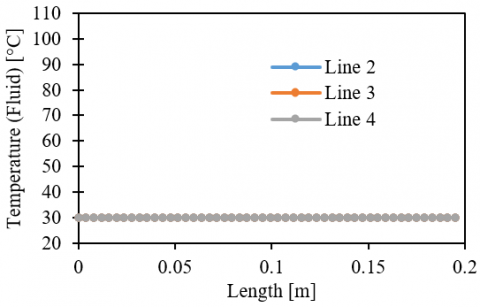
Figure 11 is the coordinate point of laminar. The average value for each distance from the center of the inner tank to the edge of the outer agitator tank. Temperature distribution data collection can be selected with four reference lines, as shown in Figure 12. Line 1 is the reference line in the center of the tank, with a length equal to 382 mm. The analysis of the simulation results with this program divided each point that determines the results of the analysis into 3 locations with reference level lines for collecting temperature distribution data, lines 2, 3, and 4, in order to be able to see the temperature effect at different heights of the agitation tank. The details of the reference levels are as follows. Line 2 is 140 mm higher than the reference line at the bottom of the agitator tank and has a length from the center of the agitator tank to the outer edge of the agitator tank equal to 195 mm. Line 4 is 340 mm above the reference line level and has a length from the center of the agitator tank to the outer edge of the tank, 195 mm. Simulating and analyzing the change in solution temperature at each level of the reference line, as shown in Figure 13, is the result of the analysis without heating and mixing the mixture inside the agitator tank.
Figure 12. Reference level line for collecting temperature distribution data
Figure 13. The change in solution temperature at each reference line level
3.4 Grid independent
Grid independence refers to the study of selecting the appropriate number of grids in computational fluid dynamics (CFD) simulations to ensure accurate results and reduce computational time. Several papers have addressed this topic such as, Siek et al. conducted a mesh independence study to simulate the resistance of a low-speed catamaran ship and found that increasing the number of grids improved the accuracy of the ship's resistance estimation [93]. Lee et al. proposed a grid independence test method that uses grid resolution based on characteristic length and uses CV (RMSE) and R2 as criteria for selecting the most appropriate grid [94]. Jin et al. investigated the importance of verifying grid independence in CFD numerical simulations of pigs and determined appropriate element partitioning conditions for air flow and temperature simulations [107]. Therefore, verifying grid independence is important for improving the reliability and accuracy of CFD simulations in various applications where increasing the number of model grids is shown in Figure 14.
Figure 14. Computation domain and grid configuration of the present study
Figure 15. Grid independent test
In this study, the elements are divided starting from 1×10⁵ to 1×10⁶ as shown in the Figure 15. The average temperature will be followed in the perforated agitator tank for 90 s at a stirring speed of 10 rpm. The stop calculation when the difference average temperature value in the agitator tank is no more than 1×10⁻³ or 0.1%. The analysis results show that when the appropriate conditions for dividing the size of the elements are changed, the average temperature does not exceed the conditions and the number of elements is approximately 7×10⁵ elements.
The time required for the test is 90 seconds with the liquid temperature at the edge of the container set to an initial value of 100°C that heat radiating from the edge of the tank into the inside of the tank. The experiments were completed with nine different conditions. Cases 1, 2, 3 were perforated impellers, Cases 4, 5, and 6 were three- blade on the top and bottom of the impeller and Cases 7, 8, 9 were helical ribbon impeller. As shown in Table 3.
Table 3. Operating conditions of the present study
|
Case Studies |
Details |
|
Case 1 |
The perforated impellers for 90 seconds at a speed of 10 rpm |
|
Case 2 |
The perforated impellers for 90 seconds at a speed of 20 rpm |
|
Case 3 |
The perforated impellers for 90 seconds at a speed of 30 rpm |
|
Case 4 |
The 3-blade on the top and bottom of the impeller for 90 seconds at a speed of 10 rpm |
|
Case 5 |
The 3-blade on the top and bottom of the impeller for 90 seconds at a speed of 20 rpm |
|
Case 6 |
The 3-blade on the top and bottom of the impeller for 90 seconds at a speed of 30 rpm |
|
Case 7 |
The Helical ribbon impeller was for 90 seconds at a speed of 10 rpm |
|
Case 8 |
The Helical ribbon impeller was for 90 seconds at a speed of 20 rpm |
|
Case 9 |
The Helical ribbon impeller was for 90 seconds at a speed of 30 rpm |
The mixing time is also an important parameter in evaluating the economic efficiency of the agitator tank and directly influences the operating cost and product quality [108]. The results of the analysis using the program use a mix of more than 90% as the maximum acceptable value for agitation. Based on average data from different locations, a level of homogeneity of 90% is considered adequate for most chemical engineering processes and systems [109].
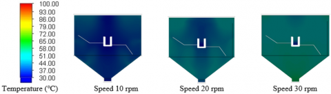
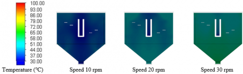
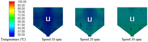
4.1 The color shades of temperature change
The color shades of temperature change can be seen in Figures 16-18. The agitating mixture in the agitator tank was agitated with three types of impellers at three different speeds at the laminar z = 0 m. Figures 16-18. found that by using the Helical ribbon impeller in Figure 18 at a speed of 30 rpm for 90 seconds, the shade of heat generated in the agitator tank can be distributed throughout the tank best when compared to other types of impellers and other speeds due to the two-paddle impeller, when it moves, the liquid flows in the direction of rotation around the impeller, which occurs on both blades, causing the liquid to swirl, resulting in uneven mixing. This is consistent with reports suggesting that the helical ribbon impeller is more effective than the pitch blade and straight blade agitator [110]. The results of the study of the perforated impeller in Figure 16 at a speed of 30 rpm found that the distribution of heat shades in the agitator tank was minimal compared to other types of impellers and other speeds.
These three types of agitator blades are commonly used due to their initial effectiveness in mixing. Therefore, they were selected for this study for the reasons mentioned above [79, 82, 83]. The temperature (color of temperature) at each position in the mixing tank indicates that while the results may not be uniformly mixed throughout the tank, they represent the best outcome among the three selected blade types. The ability to distribute evenly is crucial for effective mixing. In practical applications, it is expected that the temperature effect would be lower than in the model, as there are external factors that we may not be able to control in the analytical model. Additionally, if the raw materials used have different properties, this could further increase the margin of error in the analysis. The temperature stratification in the mixing tank could result from issues with the raw materials used in practical applications. For example, inadequate mixing in certain areas could lead to substances and raw materials getting stuck, causing errors in the mixing process. This problem could result in the agitator not performing as desired. When applied in industrial settings and at larger scales than analyzed in this article, changes in various parts of the agitator and variations in the volume of materials could alter the properties of the liquid, leading to potentially different outcomes from those predicted in this model [80].
Figure 16. The shade indicates the mixture’s temperature when using the perforated impellers for 90 seconds
Figure 17. The shade indicates the mixture’s temperature when using a 3-blade on the top and bottom of the impeller for 90 seconds
Figure 18. The shade indicates the mixture’s temperature when using the Helical ribbon impeller for 90 seconds
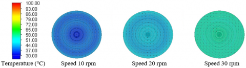
4.2 Change of mixture direction
For the direction of change of movement of the mixture, it can be shown as shown in Figures 19-21.
Figure 19. Vector and temperature showing the movement of the mixture using a perforated impeller for 90 seconds
Figure 20. Vector and temperature showing the movement of the mixture using a 3-blade on the top and bottom of the impeller for 90 seconds
Figure 21. Vector and temperature showing the movement of the mixture using the Helical ribbon impeller for 90 seconds
Vector distribution of the mixture in the flow direction along the cross-section, Analysis using the model at the plane z=0 m as shown in Figures 19-21 for all three types of impellers found that the helical ribbon impeller from Figure 21 at a speed of 30 rpm made the mixture in the agitator tank the most even vector distribution. The point at which the vector swirl occurred in the agitator tank is minimal compared to other impellers because this type of impeller allows the liquid to flow smoothly and distribute the flow from the bottom to the top and from the outside to the inside very well. It is consistent with reports of a single ribbon mixer that can create an axially symmetrical flow cell that moves liquid below the outer edge of the tank and up near the center [85]. Three blades are attached on the top and bottom of the impeller from Figure 21. at a speed of 30 rpm at a time of 90 seconds. It was found that this type of impeller causes the mixture in the agitator tank to have the least distribution of the movement vector. It is caused by the rotation of the vector in the agitator tank at many points, causing the mixing of the mixture to not be as good as it should be compared to other types of impellers.
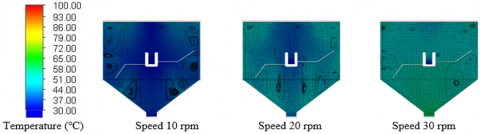
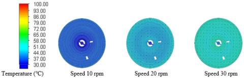
4.3 The direction of change in mixing at the Y-axis of 0 mm. and Y-axis of 90 mm
Demonstrates the change in movement of the mixture. At the Y-axis of 0 mm, as shown in Figures 22-24, and at the Y-axis of 90 mm, as shown in Figures 25-27, the agitation of the substance in the mixing tank using all three types of blades and at three different speeds is illustrated. In the Y-axis plane of 0 mm, as shown in Figure 24, the use of the ribbon blade at a speed of 30 rpm at 90 seconds yielded the best vector and temperature distribution. The temperature was most effectively distributed from the center of the tank to the tank's edges. When comparing to other blade types, in the Y-axis plane of 90 mm, as shown in Figure 27, the ribbon blade at a speed of 30 rpm at 90 seconds also yielded the best vector and temperature distribution. Similarly, the paddle blade, shown in Figure 25, at a speed of 30 rpm, resulted in the least vector and temperature distribution. The temperature was distributed least from the center of the tank to the tank's edges compared to other blade types and speeds.
Figure 22. Vector and Temperature showing the movement of the mixture using a perforated impeller for 90 seconds
Figure 23. Vector and Temperature showing the movement of the mixture using a 3-blade on the top and bottom of the impeller for 90 seconds
Figure 24. Vector and Temperature showing the movement of the mixture using the Helical ribbon impeller for 90 seconds
However, the vector distribution of the mixture in the analysis at the Y-axis of 0 mm, where the temperature was highest, was found to be most evenly distributed throughout the mixing tank. This is because there is less resistance during mixing, as there is no shear force between the material and the walls of the tank or between the ribbon blade and the tank wall. This is consistent with reports that ribbon agitators perform better than pitched blade and straight blade agitators. In the Y-axis plane of 90 mm, for all three types of blades, there was a consistent and close distribution of vector movement. The point at which the vector rotates the mixing tank occurred minimally and similarly. This is because the blades work to their full capacity, allowing the liquid to flow smoothly.
4.4 Temperature distribution results
The results from the analysis using the model as shown in Figures 19-27 can help predict the outcomes when used in actual operations. The temperature distribution results for different blade types show that the ribbon blade requires the least time to evenly distribute the temperature throughout the mixing tank. The analysis results indicate that in actual use, the ribbon blade requires the least time for mixing, leading to cost savings in terms of electrical energy and certain substances used for agitation. Prolonged agitation can lead to degradation or evaporation, resulting in inaccurate proportions. Some blade types cannot achieve uniform heat distribution within the stirrer, directly affecting the quality of the final product. In reality, prolonged use would lead to more energy and time consumption [109].
Figure 25. Vector and Temperature showing the movement of the mixture using a perforated impeller for 90 seconds
Figure 26. Vector and Temperature showing the movement of the mixture using a 3-blade on the top and bottom of the impeller for 90 seconds
Figure 27. Vector and temperature showing the movement of the mixture using the Helical ribbon impeller for 90 seconds
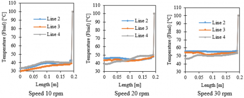
4.5 Change of temperature
It shows the temperature change of the impellers in each type by displaying the temperature change behavior of the mixture at different speeds, as shown in Figures 28-30. Changes in temperature distribution at each level of the reference line (Line 2-3-4) are used to check and average the results that occur within the agitator tank, as shown in Figures 28-30. According to the analysis of the agitator tank simulation and the three types of impellers, it was found that the helical ribbon impeller had a speed of 30 rpm for 90 seconds. In Figure 31, the temperature distribution at each level of the reference line inside the agitator tank averaged over each distance from the inner tank’s center to the outer tank’s edge, is the highest compared to other impellers. There is a minimal difference in the average temperature change in each distance from the center of the inner tank to the outer tank’s edge compared to other impeller types. From the results of the helical ribbon impeller mentioned above, it can be discussed that the heat can be distributed most evenly throughout the agitator tank from the outside to the core. Correlation with Figure 27. At 30 rpm, the temperature in the center of the mixing tank is higher, differing from the surrounding areas, and is consistent with various studies on different impeller blade designs. It was found that the radial blade impeller used in this study provides the widest area for mass transfer, and due to the smallest dead zone size, it may reduce mixing time [106, 111], thus resulting in lower energy consumption, making it the most suitable option [84].
Figure 28. The change in temperature of the perforated impeller at 90 seconds at each level of the reference line at various agitation speeds
Figure 29. The change in temperature of a 3-blade on the top and bottom of the impeller at 90 seconds at each level of the reference line at various agitation speeds
Figure 30. The change in temperature of the Helical ribbon impeller at 90 seconds at each level of the reference line at various agitation speeds
4.6 Average temperature change at all 40 points inside the agitator tank
The temperature change behavior of the fluid properties simulation inside the agitator tank is averaged at 40 points distributed throughout the model domain at 90 seconds.
Figure 31. Average temperature from 40 observation points distributed across the model domain
Analytical tests used the simulation of agitator tanks and impellers to observe the mixing of the average temperatures from zones A, B, and C of the three types of impellers at 90 seconds. Figure 31 shows that the helical ribbon impeller at a speed of 10 rpm has the highest average temperature at every point inside the agitator tank compared to other types of impellers, equal to 53.69℃. It shows that this type of impeller has the highest agitation efficiency. It is consistent with the comparison of viscosity characteristics of a mechanical agitator. It can provide the effect of homogeneous mixing for very high-viscosity liquids. Flow analysis shows that a double ribbon is the most effective [112]. The helical ribbon impeller is at a speed of 30 rpm, which is the same speed as other types of impellers. However, this impeller can achieve the best temperature distribution throughout the agitator tank and is better than the other impellers that use the same speed. It will also help reduce the electrical energy used and the time in the agitation process. This is consistent with the results of the study, which stated that agitation time and energy consumption are important parameters in evaluating the economic performance of the agitator tank because these parameters depend on the tank layout and directly influence both the operating cost and product quality [109].
This article concerns the mixing of high-viscosity fluids using close-clearance impellers in a cylindrical tank. This study was carried out through a numerical model of three different types of impellers and speeds of 10, 20, and 30 rpm, respectively. The study involved the distribution of shades within the agitator tank, the movement of vectors, the temperature of each distance from the tank’s center to the tank’s edge, and the average temperature inside the tank. Using the helical ribbon impeller at a speed of 30 rpm for 90 seconds showed that the shade of heat generated in the agitator tank can be distributed throughout the tank best compared to other impellers and speeds. According to the helical ribbon impeller, at a speed of 30 rpm at a time of 90 seconds, it found that this type of impeller caused the mixture in the agitator tank to have the most even distribution of vectors and the least amount of vector rotation in the tank when compared to other types of impellers. Regarding the helical ribbon impeller at a speed of 30 rpm at a time of 90 seconds, the temperature distribution at each level of the reference line inside the agitator tank, which is averaged over the distance from the center of the inner tank to the edge of the outer tank, is the highest compared to other types of impellers. There is a minimal difference in the average temperature change in each distance from the center of the inner tank to the outer tank’s edge compared to other impeller types. The helical ribbon impeller at a speed of 10 rpm has the highest average temperature at all points inside the agitator tank compared to other impellers, equal to 53.69℃, showing that this type of agitator has the highest agitation efficiency. Furthermore, the ribbon impeller used in this study provides the widest area for mass transfer and, due to the smallest dead zone size, may result in reduced mixing time and, consequently, lower energy consumption.
Therefore, based on the overall results of this research, it is found that the ribbon blade provides the best outcomes in terms of temperature distribution, mixing time, mixing speed, energy consumption, and overall mixing quality. However, it is important to note that these findings are based on analysis from a model. In practical applications, whether in household or industrial settings, it is necessary to control all factors as modeled. Otherwise, there may be deviations in the results. Similarly, scaling up could lead to different outcomes due to changes in various factors. Nonetheless, the researchers hope that there will be interest in furthering the use of the simulation results presented in this article for real-world applications or future testing. Comparing these results with actual experiments and further statistical analysis would help in making more accurate decisions regarding the selection of blade types and increase confidence in the results. Ultimately, this would greatly benefit the mixing process in the future.
This work was supported by the Agricultural Machinery and Postharvest Technology Innovation Center, Science, Research and Innovation Promotion and Utilization Division, Office of the Ministry of Higher Education, Science, Research and Innovation and Faculty of Engineering, Khon Kaen University. The machine learning tools of Rajamangala University of Technology Isan, Khon Kaen Campus and Nakhon Ratchasima Campus. The experiment was supported by Udonthani Rajabhat University and Agricultural Machinery and Post-Harvest Technology Center, AMPTC., Khon Kaen University.
[1] Atiwesh, G., Mikhael, A., Parrish, C.C., Banoub, J., Le, T.A.T. (2021). Environmental impact of bioplastic use: A review. Heliyon, 7(9): e07918. https://doi.org/10.1016/j.heliyon.2021.e07918
[2] Akindoyo, J.O., Beg, M., Ghazali, S., Islam, M.R., Jeyaratnam, N., Yuvaraj, A.R. (2016). Polyurethane types, synthesis and applications–A review. Rsc Advances, 6(115): 114453-114482. https://doi.org/10.1039/c6ra14525f
[3] Cocker, T.L., Jelic, V., Gupta, M., Molesky, S.J., Burgess, J.A., Reyes, G.D.L., Titova, L.V., Tsui, Y.Y., Freeman, M.R., Hegmann, F.A. (2013). An ultrafast terahertz scanning tunnelling microscope. Nature Photonics, 7(8): 620-625. https://doi.org/10.1038/nphoton.2013.151
[4] Sibaly, S., Jeetah, P. (2017). Production of paper from pineapple leaves. Journal of Environmental Chemical Engineering, 5(6): 5978-5986. https://doi.org/10.1016/j.jece.2017.11.026
[5] Vazquez-Rojas, R.A., Garfias-Vásquez, F.J., Bazua-Rueda, E.R. (2018). Simulation of a triple effect evaporator of a solution of caustic soda, sodium chloride, and sodium sulfate using Aspen Plus. Computers & Chemical Engineering, 112: 265-273. https://doi.org/10.1016/j.compchemeng.2018.02.005
[6] Boadu, K.B., Kyenkyehene, H.K., Anokye, R. (2023). Evaluation of physico-mechanical properties and biodegradability of plant containers made from biomaterials for sustainable agriculture. Journal of Agricultural Research, 61(3): 219-228. https://doi.org/10.58475/2023.61.3.1977
[7] Jahroo, W.L., CA, M.D., Sakina, S.I. (2021). Biodegradable food container made of abaca fiber pulp with beeswax biocoating. In ICON ARCCADE 2021: The 2nd International Conference on Art, Craft, Culture and Design (ICON-ARCCADE 2021), pp. 195-200. https://doi.org/10.2991/assehr.k.211228.025
[8] Devi, T.T., Kumar, B. (2013). CFD simulation of flow patterns in dual impeller stirred tank. International Journal of Modelling and Simulation, 33(2): 117-125. https://doi.org/10.2316/Journal.205.2013.2.205-5776
[9] Stuparu, A., Susan-Resiga, R., Bosioc, A. (2021). CFD simulation of solid suspension for a liquid–solid industrial stirred reactor. Applied Sciences, 11(12): 5705. https://doi.org/10.3390/app11125705
[10] Mao, Z., Yang, C. (2017). Micro-mixing in chemical reactors: A perspective. Chinese Journal of Chemical Engineering, 25(4): 381-390. https://doi.org/10.1016/j.cjche.2016.09.012
[11] Kresta, S.M., Etchells III, A.W., Dickey, D.S., Atiemo-Obeng, V.A. (2015). Advances in industrial mixing: A companion to the handbook of industrial mixing. John Wiley & Sons. https://doi.org/10.1595/205651317x696225
[12] Heidari, A. (2020). CFD simulation of impeller shape effect on quality of mixing in two-phase gas–liquid agitated vessel. Chinese Journal of Chemical Engineering, 28(11): 2733-2745. https://doi.org/10.1016/j.cjche.2020.06.036
[13] Trad, Z., Fontaine, J.P., Larroche, C., Vial, C. (2017). Experimental and numerical investigation of hydrodynamics and mixing in a dual-impeller mechanically-stirred digester. Chemical Engineering Journal, 329: 142-155. https://doi.org/10.1016/j.cej.2017.07.038
[14] Coroneo, M., Montante, G., Paglianti, A., Magelli, F. (2011). CFD prediction of fluid flow and mixing in stirred tanks: Numerical issues about the RANS simulations. Computers & Chemical Engineering, 35(10): 1959-1968. https://doi.org/10.1016/j.compchemeng.2010.12.007
[15] Yamamoto, T., Fang, Y., Komarov, S.V. (2019). Surface vortex formation and free surface deformation in an unbaffled vessel stirred by on-axis and eccentric impellers. Chemical Engineering Journal, 367: 25-36. https://doi.org/10.1016/j.cej.2019.02.130
[16] Taghavi, M., Zadghaffari, R., Moghaddas, J., Moghaddas, Y. (2011). Experimental and CFD investigation of power consumption in a dual Rushton turbine stirred tank. Chemical Engineering Research and Design, 89(3): 280-290. https://doi.org/10.1016/j.cherd.2010.07.006
[17] Gabriele, A., Nienow, A.W., Simmons, M.J.H. (2009). Use of angle resolved PIV to estimate local specific energy dissipation rates for up-and down-pumping pitched blade agitators in a stirred tank. Chemical Engineering Science, 64(1): 126-143. https://doi.org/10.1016/j.ces.2008.09.018
[18] de Lamotte, A., Delafosse, A., Calvo, S., Toye, D. (2018). Identifying dominant spatial and time characteristics of flow dynamics within free-surface baffled stirred-tanks from CFD simulations. Chemical Engineering Science, 192: 128-142. https://doi.org/10.1016/j.ces.2018.07.024
[19] Cheng, J.C., Fox, R.O. (2010). Kinetic modeling of nanoprecipitation using CFD coupled with a population balance. Industrial & Engineering Chemistry Research, 49(21): 10651-10662. https://doi.org/10.1021/ie100558n
[20] Haringa, C., Noorman, H.J., Mudde, R.F. (2017). Lagrangian modeling of hydrodynamic–Kinetic interactions in (bio) chemical reactors: Practical implementation and setup guidelines. Chemical Engineering Science, 157: 159-168. https://doi.org/10.1016/j.ces.2016.07.031
[21] Morchain, J., Gabelle, J.C., Cockx, A. (2014). A coupled population balance model and CFD approach for the simulation of mixing issues in lab-scale and industrial bioreactors. AIChE Journal, 60(1): 27-40. https://doi.org/10.1002/aic.14238
[22] Lane, G.L. (2017). Improving the accuracy of CFD predictions of turbulence in a tank stirred by a hydrofoil impeller. Chemical Engineering Science, 169: 188-211. https://doi.org/10.1016/j.ces.2017.03.061
[23] Ranganathan, P., Sivaraman, S. (2011). Investigations on hydrodynamics and mass transfer in gas–Liquid stirred reactor using computational fluid dynamics. Chemical Engineering Science, 66(14): 3108-3124. https://doi.org/10.1016/j.ces.2011.03.007
[24] Visscher, F., Van der Schaaf, J., Nijhuis, T.A., Schouten, J.C. (2013). Rotating reactors–A review. Chemical Engineering Research and Design, 91(10): 1923-1940. https://doi.org/10.1016/j.cherd.2013.07.021
[25] Alcamo, R., Micale, G., Grisafi, F., Brucato, A., Ciofalo, M. (2005). Large-eddy simulation of turbulent flow in an unbaffled stirred tank driven by a Rushton turbine. Chemical Engineering Science, 60(8-9): 2303-2316. https://doi.org/10.1016/j.ces.2004.11.017
[26] Zadghaffari, R., Moghaddas, J.S., Revstedt, J. (2010). Large-eddy simulation of turbulent flow in a stirred tank driven by a Rushton turbine. Computers & Fluids, 39(7): 1183-1190. https://doi.org/10.1016/j.compfluid.2010.03.001
[27] Lee, K., Huque, Z., Kommalapati, R., Han, S.E. (2017). Fluid-structure interaction analysis of NREL phase VI wind turbine: Aerodynamic force evaluation and structural analysis using FSI analysis. Renewable Energy, 113: 512-531. https://doi.org/10.1016/j.renene.2017.02.071
[28] Lozovskiy, A., Olshanskii, M.A., Vassilevski, Y.V. (2019). Analysis and assessment of a monolithic FSI finite element method. Computers & Fluids, 179: 277-288. https://doi.org/10.1016/j.compfluid.2018.11.004
[29] Piatti, F., Sturla, F., Marom, G., Sheriff, J., Claiborne, T. E., Slepian, M.J., Redaelli, A., Bluestein, D. (2015). Hemodynamic and thrombogenic analysis of a trileaflet polymeric valve using a fluid–Structure interaction approach. Journal of Biomechanics, 48(13): 3641-3649. https://doi.org/10.1016/j.jbiomech.2015.08.009
[30] Wang, L., Quant, R., Kolios, A. (2016). Fluid structure interaction modelling of horizontal-axis wind turbine blades based on CFD and FEA. Journal of Wind Engineering and Industrial Aerodynamics, 158: 11-25. https://doi.org/10.1016/j.jweia.2016.09.006
[31] Hermange, C., Oger, G., Le Chenadec, Y., Le Touzé, D. (2019). A 3D SPH–FE coupling for FSI problems and its application to tire hydroplaning simulations on rough ground. Computer Methods in Applied Mechanics and Engineering, 355: 558-590. https://doi.org/10.1016/j.cma.2019.06.033
[32] Han, H., Yu, R., Li, B., Zhang, Y., Wang, W., Chen, X. (2019). Multi-objective optimization of corrugated tube with loose-fit twisted tape using RSM and NSGA-II. International Journal of Heat and Mass Transfer, 131: 781-794. https://doi.org/10.1016/j.ijheatmasstransfer.2018.10.128
[33] Chen, X., Yao, J., Jiang, S. C., Liu, C., Guo, M., Gao, N., Zhang, Z. (2020). An improved CFD modeling approach applied for the simulation of gas–Liquid interaction in the ozone contactor along with structure optimization. Chemical Engineering Journal, 384: 123322. https://doi.org/10.1016/j.cej.2019.123322
[34] Na, J., Kshetrimayum, K.S., Lee, U., Han, C. (2017). Multi-objective optimization of microchannel reactor for Fischer-Tropsch synthesis using computational fluid dynamics and genetic algorithm. Chemical Engineering Journal, 313: 1521-1534. https://doi.org/10.1016/j.cej.2016.11.040
[35] Zhu, B., Wang, X., Tan, L., Zhou, D., Zhao, Y., Cao, S. (2015). Optimization design of a reversible pump–turbine runner with high efficiency and stability. Renewable Energy, 81: 366-376. https://doi.org/10.1016/j.renene.2015.03.050
[36] Poojeera, S., Srichat, A., Naphon, N., Naphon, P. (2022). Study on thermal performance of the small-scale air conditioning with thermoelectric cooling module. Mathematical Modelling of Engineering Problems, 9(4): 1143-1151. https://doi.org/10.18280/mmep.090434
[37] Wangkahart, S., Junsiri, C., Srichat, A., Poojeera, S., Laloon, K., Hongtong, K., Boupha, P. (2022). Using greenhouse modelling to identify the optimal conditions for growing crops in northeastern Thailand. Mathematical Modelling of Engineering Problems, 9(6): 1648-1658. https://doi.org/10.18280/mmep.090626
[38] Srichat, A., Vengsungnle, P., Bootwong, A., Poojeera, S., Naphon, P. (2021). Study on thermal efficiency of salt incubator with waste heat recovery in the rock salt boiling process. International Journal of Heat & Technology, 39(6): 1733-1740. https://doi.org/10.18280/ijht.390605
[39] Singh, H., Fletcher, D.F., Nijdam, J.J. (2011). An assessment of different turbulence models for predicting flow in a baffled tank stirred with a Rushton turbine. Chemical Engineering Science, 66(23): 5976-5988. https://doi.org/10.1016/j.ces.2011.08.018
[40] Joshi, J.B., Nere, N.K., Rane, C.V., Murthy, B.N., Mathpati, C.S., Patwardhan, A.W., Ranade V.V. (2011). CFD simulation of stirred tanks: Comparison of turbulence models. Part I: Radial flow impellers. The Canadian Journal of Chemical Engineering, 89(1): 23-82. https://doi.org/10.1002/cjce.20446
[41] Sossa-Echeverria, J., Taghipour, F. (2015). Computational simulation of mixing flow of shear thinning non-Newtonian fluids with various impellers in a stirred tank. Chemical Engineering and Processing: Process Intensification, 93: 66-78. https://doi.org/10.1016/j.cep.2015.04.009
[42] Zhang, B., Liang, C. (2015). A simple, efficient, and high-order accurate curved sliding-mesh interface approach to spectral difference method on coupled rotating and stationary domains. Journal of Computational Physics, 295: 147-160. https://doi.org/10.1016/j.jcp.2015.04.006
[43] Santos-Moreau, V., Brunet-Errard, L., Rolland, M. (2012). Numerical CFD simulation of a batch stirred tank reactor with stationary catalytic basket. Chemical Engineering Journal, 207: 596-606. https://doi.org/10.1016/j.cej.2012.07.020
[44] Hoseini, S.S., Najafi, G., Ghobadian, B., Akbarzadeh, A.H. (2021). Impeller shape-optimization of stirred-tank reactor: CFD and fluid structure interaction analyses. Chemical Engineering Journal, 413: 127497. https://doi.org/10.1016/j.cej.2020.127497
[45] Valizadeh, K., Farahbakhsh, S., Bateni, A., Zargarian, A., Davarpanah, A., Alizadeh, A., Zarei, M. (2020). A parametric study to simulate the non-Newtonian turbulent flow in spiral tubes. Energy Science & Engineering, 8(1): 134-149. https://doi.org/10.1002/ese3.514
[46] Stuparu, A., Susan-Resiga, R., Tanasa, C. (2021). CFD assessment of the hydrodynamic performance of two impellers for a baffled stirred reactor. Applied Sciences, 11(11): 4949. https://doi.org/10.3390/app11114949
[47] Stuparu, A., Susan-Resiga, R., Bosioc, A. (2021). Improving the homogenization of the liquid-solid mixture using a tandem of impellers in a baffled industrial reactor. Applied Sciences, 11(12): 5492. https://doi.org/10.3390/app11125492
[48] Stachnik, M., Jakubowski, M. (2020). Multiphase model of flow and separation phases in a whirlpool: Advanced simulation and phenomena visualization approach. Journal of Food Engineering, 274: 109846. https://doi.org/10.1016/j.jfoodeng.2019.109846
[49] Tembely, M., Alameri, W.S., AlSumaiti, A.M., Jouini, M.S. (2020). Pore-scale modeling of the effect of wettability on two-phase flow properties for Newtonian and non-Newtonian fluids. Polymers, 12(12): 2832. https://doi.org/10.3390/polym12122832
[50] McCraney, J., Weislogel, M., Steen, P. (2020). OpenFOAM simulations of late stage container draining in microgravity. Fluids, 5(4): 207. https://doi.org/10.3390/fluids5040207
[51] He, X., Xu, H., Li, W., Sheng, D. (2020). An improved VOF-DEM model for soil-water interaction with particle size scaling. Computers and Geotechnics, 128: 103818. https://doi.org/10.1016/j.compgeo.2020.103818
[52] Silva, M.F., Campos, J.B., Miranda, J.M., Araújo, J.D. (2020). Numerical study of single Taylor bubble movement through a microchannel using different CFD packages. Processes, 8(11): 1418. https://doi.org/10.3390/pr8111418
[53] Anton, A., Cretu, V. I., Ruprecht, A., Muntean, S. (2013). Traffic replay compression (TRC): A highly efficient method for handling parallel numerical simulation data. In Proceedings of the Romanian Academy, Series A, 14: 385-392.
[54] Anton, A. (2016). Numerical investigation of unsteady flows using OpenFOAM. Hidraulica, 1: 7.
[55] Blais, B., Bertrand, F. (2017). CFD-DEM investigation of viscous solid–liquid mixing: Impact of particle properties and mixer characteristics. Chemical Engineering Research and Design, 118: 270-285. https://doi.org/10.1016/j.cherd.2016.12.018
[56] Tamburini, A., Cipollina, A., Micale, G., Brucato, A., Ciofalo, M. (2013). CFD simulations of dense solid–Liquid suspensions in baffled stirred tanks: Prediction of solid particle distribution. Chemical Engineering Journal, 223: 875-890. https://doi.org/10.1016/j.cej.2013.03.048
[57] Buffo, A., Vanni, M., Marchisio, D.L. (2012). Multidimensional population balance model for the simulation of turbulent gas–Liquid systems in stirred tank reactors. Chemical Engineering Science, 70: 31-44. https://doi.org/10.1016/j.ces.2011.04.042
[58] Ochieng, A., Onyango, M.S. (2008). Drag models, solids concentration and velocity distribution in a stirred tank. Powder Technology, 181(1): 1-8. https://doi.org/10.1016/j.powtec.2007.03.034
[59] Montante, G., Magelli, F. (2007). Mixed solids distribution in stirred vessels: Experiments and computational fluid dynamics simulations. Industrial & Engineering Chemistry Research, 46(9): 2885-2891. https://doi.org/10.1021/ie060616i
[60] Lane, G.L., Schwarz, M.P., Evans, G.M. (2005). Numerical modelling of gas–Liquid flow in stirred tanks. Chemical Engineering Science, 60(8-9): 2203-2214. https://doi.org/10.1016/j.ces.2004.11.046
[61] Khopkar, A.R., Ranade, V.V. (2006). CFD simulation of gas–liquid stirred vessel: VC, S33, and L33 flow regimes. AIChE Journal, 52(5): 1654-1672. https://doi.org/10.1002/aic.10762
[62] Joshi, J.B., Nere, N.K., Rane, C.V., Murthy, B.N., Mathpati, C.S., Patwardhan, A.W., Ranade, V.V. (2011). CFD simulation of stirred tanks: Comparison of turbulence models (Part II: Axial flow impellers, multiple impellers and multiphase dispersions). The Canadian Journal of Chemical Engineering, 89(4): 754-816. https://doi.org/10.1002/cjce.20465
[63] Derksen, J.J. (2006). Long-time solids suspension simulations by means of a large-eddy approach. Chemical Engineering Research and Design, 84(1): 38-46. https://doi.org/10.1205/cherd.05069
[64] Derksen, J.J. (2003). Numerical simulation of solids suspension in a stirred tank. AIChE Journal, 49(11): 2700-2714. https://doi.org/10.1002/aic.690491104
[65] Sbrizzai, F., Lavezzo, V., Verzicco, R., Campolo, M., Soldati, A. (2006). Direct numerical simulation of turbulent particle dispersion in an unbaffled stirred-tank reactor. Chemical Engineering Science, 61(9): 2843-2851. https://doi.org/10.1016/j.ces.2005.10.073
[66] Feng, X., Cheng, J., Li, X., Yang, C., Mao, Z.S. (2012). Numerical simulation of turbulent flow in a baffled stirred tank with an explicit algebraic stress model. Chemical Engineering Science, 69(1): 30-44. https://doi.org/10.1016/j.ces.2011.09.055
[67] Zamiri, A., Chung, J.T. (2018). Numerical evaluation of turbulent flow structures in a stirred tank with a Rushton turbine based on scale-adaptive simulation. Computers & Fluids, 170: 236-248. https://doi.org/10.1016/j.compfluid.2018.05.007
[68] Blais, B., Lassaigne, M., Goniva, C., Fradette, L., Bertrand, F. (2016). A semi-implicit immersed boundary method and its application to viscous mixing. Computers & Chemical Engineering, 85: 136-146. https://doi.org/10.1016/j.compchemeng.2015.10.019
[69] Malik, S., Lévêque, E., Bouaifi, M., Gamet, L., Flottes, E., Simoëns, S., El-Hajem, M. (2016). Shear improved Smagorinsky model for large eddy simulation of flow in a stirred tank with a Rushton disk turbine. Chemical Engineering Research and Design, 108: 69-80. https://doi.org/10.1016/j.cherd.2016.02.035
[70] Weheliye, W.H., Cagney, N., Rodriguez, G., Micheletti, M., Ducci, A. (2018). Mode decomposition and Lagrangian structures of the flow dynamics in orbitally shaken bioreactors. Physics of Fluids, 30(3). https://doi.org/10.1063/1.5016305
[71] Sakowitz, A., Mihaescu, M., Fuchs, L. (2014). Flow decomposition methods applied to the flow in an IC engine manifold. Applied Thermal Engineering, 65(1-2): 57-65. https://doi.org/10.1016/j.applthermaleng.2013.12.082
[72] Semeraro, O., Bellani, G., Lundell, F. (2012). Analysis of time-resolved PIV measurements of a confined turbulent jet using POD and Koopman modes. Experiments in Fluids, 53: 1203-1220. https://doi.org/10.1007/s00348-012-1354-9
[73] de Lamotte, A., Delafosse, A., Calvo, S., Delvigne, F., Toye, D. (2017). Investigating the effects of hydrodynamics and mixing on mass transfer through the free-surface in stirred tank bioreactors. Chemical Engineering Science, 172: 125-142. https://doi.org/10.1016/j.ces.2017.06.028
[74] Brucato, A., Ciofalo, M., Grisafi, F., Tocco, R. (2000). On the simulation of stirred tank reactors via computational fluid dynamics. Chemical Engineering Science, 55(2): 291-302. https://doi.org/10.1016/S0009-2509(99)00324-3
[75] Zhang, Y., Yu, G., Yu, L., Siddhu, M.A.H., Gao, M., Abdeltawab, A.A., Al-Deyab, S.S., Chen, X. (2016). Computational fluid dynamics study on mixing mode and power consumption in anaerobic mono-and co-digestion. Bioresource Technology, 203: 166-172. https://doi.org/10.1016/j.biortech.2015.12.023
[76] Ge, M., Chen, J., Zhao, L., Zheng, G. (2023). Mixing transport mechanism of three-phase particle flow based on CFD-DEM coupling. Processes, 11(6): 1619. https://doi.org/10.3390/pr11061619
[77] Moghbeli, M.R., Namayandeh, S., Hashemabadi, S.H. (2010). Wet hydrolysis of waste polyethylene terephthalate thermoplastic resin with sulfuric acid and CFD simulation for high viscous liquid mixing. International Journal of Chemical Reactor Engineering, 8(1). https://doi.org/10.2202/1542-6580.2240
[78] Basheer, A.A., Subramaniam, P. (2012). Hydrodynamics, mixing and selectivity in a partitioned bubble column. Chemical Engineering Journal, 187: 261-274. https://doi.org/10.1016/j.cej.2012.01.078
[79] Hadjeb, A., Bouzit, M., Kamla, Y., Ameur, H. (2017). A new geometrical model for mixing of highly viscous fluids by combining two-blade and helical screw agitators. Polish Journal of Chemical Technology, 19(3): 83-91. https://doi.org/10.1515/pjct-2017-0053
[80] Rajasekaran, E., Kumar, B., Muruganandhan, R., Raman, S.V., Antony, U. (2018). Determination of forced convection heat transfer coefficients and development of empirical correlations for milk in vessel with mechanical agitators. Journal of Food Science and Technology, 55: 2514-2522. https://doi.org/10.1007/s13197-018-3169-z
[81] Tsui, Y.Y., Hu, Y.C. (2011). Flow characteristics in mixers agitated by helical ribbon blade impeller. Engineering Applications of Computational Fluid Mechanics, 5(3): 416-429. https://doi.org/10.1080/19942060.2011.11015383
[82] Liu, B., Zheng, Y., Cheng, R., Xu, Z., Wang, M., Jin, Z. (2018). Experimental study on gas–liquid dispersion and mass transfer in shear-thinning system with coaxial mixer. Chinese Journal of Chemical Engineering, 26(9): 1785-1791. https://doi.org/10.1016/j.cjche.2018.02.009
[83] Ceres, D., Jirout, T., Rieger, F. (2010). Pitched blade turbine efficiency at particle suspension. Acta Polytechnica, 50(6): 13-15. https://doi.org/10.14311/1281
[84] Hosseini, M., Nikbakht, A.M., Tabatabaei, M. (2012). Biodiesel production in batch tank reactor equipped to helical ribbon-like agitator. Modern Applied Science, 6(3): 40-45. https://doi.org/10.5539/mas.v6n3p40
[85] Robinson, M., Cleary, P.W. (2012). Flow and mixing performance in helical ribbon mixers. Chemical Engineering Science, 84: 382-398. https://doi.org/10.1016/j.ces.2012.08.044
[86] Giusteri, G.G., Seto, R. (2018). A theoretical framework for steady-state rheometry in generic flow conditions. Journal of Rheology, 62(3): 713-723. https://doi.org/10.1122/1.4986840
[87] Chen, D., Lin, J. (2022). Steady state of motion of two particles in Poiseuille flow of power-law fluid. Polymers, 14(12): 2368. https://doi.org/10.3390/polym14122368
[88] Stiles, P.J., Fletcher, D.F. (2003). Effects of gravity on the steady state of a reaction in a liquid-state microreactor—Deviations from Poiseuille flow. Physical Chemistry Chemical Physics, 5(6): 1219-1224. https://doi.org/10.1039/b211686c
[89] Low, B.C., Egan, A.K. (2014). Steady fall of isothermal, resistive-viscous, compressible fluid across magnetic field. Physics of Plasmas, 21(6): 062105. https://doi.org/10.1063/1.4882676
[90] Stiles, P.J., Fletcher, D.F., Morris, I. (2001). The effect of gravity on the rates of simple liquid-state reactions in a small, unstirred cylindrical vessel. Part II. Physical Chemistry Chemical Physics, 3(17): 3651-3655. https://doi.org/10.1039/B103123F
[91] Hacker, J.N., Linden, P.F. (2002). Gravity currents in rotating channels. Part 1. Steady-state theory. Journal of Fluid Mechanics, 457: 295-324. https://doi.org/10.1017/S0022112001007662
[92] Zhang, J., Dai, Z., Li, R., Deng, L., Liu, J., Zhou, N. (2023). Acceleration of a production-level unstructured grid finite volume CFD code on GPU. Applied Sciences, 13(10): 6193. https://doi.org/10.3390/app13106193
[93] Siek, H.C., Kader, A.S.A., Siow, C.L. (2023). Grid independence study of low speed catamaran operate in shallow water. In AIP Conference Proceedings, 2484: 2-5. https://doi.org/10.1063/5.0111116
[94] Lee, M., Park, G., Park, C., Kim, C. (2020). Improvement of grid independence test for computational fluid dynamics model of building based on grid resolution. Advances in Civil Engineering, 2020(1): 8827936. https://doi.org/10.1155/2020/8827936
[95] Williams, J., Sarofeen, C., Shan, H., Conley, M. (2016). An accelerated iterative linear solver with GPUs for CFD calculations of unstructured grids. Procedia Computer Science, 80: 1291-1300. https://doi.org/10.1016/j.procs.2016.05.504
[96] Wang, J., Sheng, C. (2014). Validations of a local correlation-based transition model using an unstructured grid CFD solver. In 7th AIAA Theoretical Fluid Mechanics Conference, p. 2211. https://doi.org/10.2514/6.2014-2211
[97] Yang, H.Q. (2010). Reduced order method for deforming unstructured grid in CFD. In 40th Fluid Dynamics Conference and Exhibit, p. 4617. https://doi.org/10.2514/6.2010-4617
[98] Corrigan, A., Camelli, F.F., Löhner, R., Wallin, J. (2011). Running unstructured grid‐based CFD solvers on modern graphics hardware. International Journal for Numerical Methods in Fluids, 66(2): 221-229. https://doi.org/10.1002/fld.2254
[99] Rane, S., Kovačević, A., Stošić, N. (2015). Analytical Grid Generation for accurate representation of clearances in CFD for Screw Machines. In IOP Conference Series: Materials Science and Engineering, 90: 012008. https://doi.org/10.1088/1757-899X/90/1/012008
[100] Kolmogorov, D.K., Shen, W.Z., Sørensen, N.N., Sørensen, J.N. (2014). Fully consistent CFD methods for incompressible flow computations. Journal of Physics: Conference Series, 524(1): 012128. https://doi.org/10.1088/1742-6596/524/1/012128.
[101] Yue, X., Shi, Y. (2023). Flow characteristics analysis of a new combination agitator based on CFD. Academic Journal of Science and Technology, 5(1): 120-125. https://doi.org/10.54097/ajst.v5i1.5469
[102] Yin, Z., Sneeuw, N. (2021). Modeling the gravitational field by using CFD techniques. Journal of Geodesy, 95(6): 68. https://doi.org/10.1007/s00190-021-01504-w
[103] Bartosik, A. (2021). Numerical modelling of heat transfer in fine dispersive slurry flow. Energies, 14(16): 4909. https://doi.org/10.3390/en14164909
[104] Trias Miquel, F.X., Álvarez Farré, X., Alsalti Baldellou, À., Gorobets, A., Oliva Llena, A. (2022). DNS and LES on unstructured grids: Playing with matrices to preserve symmetries using a minimal set of algebraic kernels. In Collection of Papers Presented at the 8th European Congress on Computational Methods in Applied Sciences and Engineering (ECCOMAS Congress 2022). Scipedia, p. 108230. https://doi.org/10.23967/eccomas.2022.096
[105] Michelassi, V. (2020). Turbomachinery research and design: The role of DNS and LES in industry. In Progress in Hybrid RANS-LES Modelling: Papers Contributed to the 7th Symposium on Hybrid RANS-LES Methods, Berlin, Germany, pp. 55-69. https://doi.org/10.1007/978-3-030-27607-2_4
[106] Ameur, H., Kamla, Y., Sahel, D. (2018). Performance of helical ribbon and screw impellers for mixing viscous fluids in cylindrical reactors. ChemEngineering, 2(2): 26. https://doi.org/10.3390/chemengineering2020026
[107] Caines, A., Ghosh, A., Bhattacharjee, A., Feldman, A. (2021). The grid independence of an electric vehicle charging station with solar and storage. Electronics, 10(23): 2940. https://doi.org/10.3390/electronics10232940
[108] Kordas, M., Story, G., Konopacki, M., Rakoczy, R. (2013). Study of mixing time in a liquid vessel with rotating and reciprocating agitator. Industrial & Engineering Chemistry Research, 52(38): 13818-13828. https://doi.org/10.1021/ie303086r
[109] Ochieng, A., Onyango, M.S. (2008). Homogenization energy in a stirred tank. Chemical Engineering and Processing: Process Intensification, 47(9-10): 1853-1860. https://doi.org/10.1016/j.cep.2007.10.014
[110] Bai, L., Zheng, Q.J., Yu, A.B. (2017). FEM simulation of particle flow and convective mixing in a cylindrical bladed mixer. Powder Technology, 313: 175-183. https://doi.org/10.1016/j.powtec.2017.03.018
[111] Yu, L., Ma, J., Chen, S. (2011). Numerical simulation of mechanical mixing in high solid anaerobic digester. Bioresource Technology, 102(2): 1012-1018. https://doi.org/10.1016/j.biortech.2010.09.079
[112] Iranshahi, A., Heniche, M., Bertrand, F., Tanguy, P. A. (2006). Numerical investigation of the mixing efficiency of the Ekato Paravisc impeller. Chemical Engineering Science, 61(8): 2609-2617. https://doi.org/10.1016/j.ces.2005.11.032