Yudha Alif Auliya*![]() | Isti Fadah
| Isti Fadah![]() | Yustri Baihaqi | Intan Nurul Awwaliyah
| Yustri Baihaqi | Intan Nurul Awwaliyah![]()
© 2024 The authors. This article is published by IIETA and is licensed under the CC BY 4.0 license (http://creativecommons.org/licenses/by/4.0/).
OPEN ACCESS
The main issue faced by coffee growers is the lack of accuracy in manual sorting. Green Bean photos are classified into three categories (dark, green, light) using the convolutional neural network approach. This study employs 360 datasets, each consisting of 120 data points per class. The CNN model uses a 512×512×3 image as its input. The number three represents the use of three specific channels: red, green, and blue. RGB is an acronym that represents the colors Red, Green, and Blue. During the feature learning phase, the input image is subjected to conversion and pooling processes. The convolutions exhibit variations in the utilization of filters and kernel sizes. The model was developed utilizing the relay activation function and pooling techniques. The dropout technique entails transforming the feature maps derived from the pooling layer into a vector shape by flattening them. This study utilized three data scenarios: 70:30, 80:20, and 90:10. The number of epochs used for each scenario was 30. This analysis compared the performance of three optimization algorithms: Adam, RMSprop, and Nadam. The optimization model using Adam with a parameter of Epoch 30 and a data scenario of 80:20 achieved the highest accuracy result of 81.67%.
classification, coffee beans, convolutional neural network, Adam’s optimization
Green beans, one of Indonesia's key exports, are currently experiencing a fall in demand. This might be attributed to the inconsistent quality of the exported green beans, which undermines the competitiveness of Indonesian exports. Ketakasi Cooperation, our study partner, is a prominent coffee exporter in the Jember District. The coffee plantation property under management spans a total area of 623 hectares. An average co-operative has the capacity to yield 10-12 tons of coffee per hectare. The annual harvest amounts to 1.560 tons [1]. An issue frequently encountered in enterprises is the scarcity of individuals possessing expertise in assessing the quality of coffee seeds. Many people experience the drawback of lengthy sorting processes, which can lead to worker fatigue and decreased accuracy.
Roasting is a crucial phase in coffee production that seeks to convert raw coffee seeds into fully prepared coffee beans. The technique entails subjecting coffee beans to temperatures ranging from 180℃ to 240℃, depending on the desired level of roast, which can vary from light, medium, to dark roast. Throughout the roasting process, coffee seeds undergo substantial chemical transformations. The amino acids and sugars present in the coffee seeds undergo reactions, resulting in the creation of several new compounds through the Maillard and caramelization processes. These activities are responsible for the distinctive aroma and flavor that coffee possesses [2].
The categorization of coffee beans after they have been roasted has become essential to ensure consistency in the quality of the coffee that is produced. Manufacturers may guarantee consistent flavor and aroma for consumers by categorizing coffee seeds based on roast level and quality, thereby ensuring that each batch of coffee fulfills the predetermined quality criteria. Post-roasting classification enables coffee manufacturers to categorize coffee seeds that have been either over or under-roasted, a factor that can have a substantial impact on the ultimate flavor characteristics of the product [3]. Therefore, this classification is an essential measure in ensuring the uniformity and excellence of coffee products available in the market.
The quality of post-roasted green beans can be categorized based on their purity and color. The quality of a good green bean can be determined by its high purity, which is indicated by its vibrant color and absence of any symptoms of damage. By considering these aspects, green beans can be categorized into three primary qualities: dark, green, and light. An issue frequently encountered with the Ketakasi Cooperation is the constraint on the experts' ability to categorize the level of ripeness of coffee beans after they have been roasted. The market demand for post-roasted green beans, particularly among coffee firms, exhibits significant variation [4]. There are companies who want medium or dark grade. Manual classification is challenging due to the difficulty in differentiating between groupings of coffee beans that encompass several grades such as grey, light, medium, and dark. Currently, there is a tool available in the market for categorizing coffee seeds after they have been roasted. However, the high price of this tool makes it challenging for farmers to afford. The issue can be resolved by the utilization of computer vision technology that can rapidly and precisely determine the grade of green beans. Prior studies have conducted study on the categorization of Green Beans using computer Vision. The study employed digital photographs to classify coffee seeds based on their RGB (red, green, blue) and HSV (hue, saturation, value) color values [5].
This research is distinguished by the inclusion of objects, datasets, and classes. Researchers aim to enhance accuracy by modifying the data scenario and adjusting the number of epochs. The CNN approach is now one of the most effective deep learning algorithms for image recognition, yielding superior results [6]. CNN consists of numerous crucial components, specifically convolution layers and pooling layers. Some of these components will be organized into a deep network architecture and model. A convolution layer is composed of numerous weights, while a pooling layer selects a sample output from a convolution layer to decrease the data rate of the preceding layer [7]. This study conducted a comparison of image classification for post-roasting coffee beans using a Convolutional Neural Network (CNN) that was enhanced using three optimization algorithms: Adam, RMSProp, and Nadam [8]. The efficacy of the developed model was evaluated using the Confusion matrix. Model testing is conducted to determine the ideal settings for CNN parameters, such as epoch and data separation sets.
The CNN method is a deep learning technique employed for autonomous learning processes in the domains of object recognition, categorization, and feature extraction. High resolution images with nonparametric distribution models demonstrate notable effectiveness [9]. The CNN method outperforms in image recognition by replicating the image identification system of the human visual cortex, allowing for efficient processing of image information [10]. The CNN method has been extensively researched by scholars for the classification of plants in high-resolution images [11].
This study examines image-based detection, specifically the classification of images using the convolutional neural network (CNN) technique. The dataset consisted of 400 images, with 80% assigned for training purposes and the remaining 20% designated for testing. The study's findings are classified into three distinct categories. The employed CNN model comprises three convolutional layers. The model underwent 10 epochs of training, utilizing a learning rate of 0.001. The model demonstrated satisfactory performance, achieving a validation precision of 0.92 and a loss value of 0.21. The study attained a training accuracy of 98% and a model testing accuracy of 76%.
Further investigation was carried out by Yanto et al. [12]. This study seeks to evaluate and compare the performance of two architectures, EfficientNetB1 and EfficientNetB0, in conjunction with two optimizers, RMSprop and SGD optimizer. The dataset comprises 8976 images, classified into 6 distinct categories. The data scenarios are divided into a ratio of 7:1:2. The results demonstrate that the EfficienteNetB0 and EfficienceNetB1 models achieved the highest accuracy rates of 0.9955 and 0.9949, respectively, with the utilization of the RMSProp optimization technique. The optimization of EfficientNetB0 resulted in an accuracy of 0.918, whereas EfficientNetB1 achieved an accuracy of 0.9079 when compared to using SGD.
This study investigates the application of the CNN method for classifying the maturity of sweet orange fruit using color brightness levels [13]. The CNN model utilizes a solitary convolutional layer. The dataset comprises 100 images classified into two distinct categories. The training process yielded a plot loss value of 0.1563. The dataset used for training and testing comprised 250 data points. The training data achieved an accuracy of 96%, while the test data achieved an accuracy of 92%. The training process terminated after 50 epochs. This study's findings effectively differentiate the orange fruit with accuracy.
A follow-up study was conducted by LeCun and Bengio [14] entitled "Plasmodium Parasite Detection on Microscopic Imaging of Blood Removal with Deep Learning Methods." This study investigates the origins and causes of malaria. The CNN architecture uses a three-layer convolutional structure and is trained on a dataset of 27,560 images divided into two classes. The CNN model underwent evaluation with multiple optimization algorithms, such as Adam, Nadam, SGD, RMSProp, Adamax, AdaDelta, and AdaGrad. Adam optimization achieved a peak accuracy of 99.18%. The study utilized a CNN model with an image input size of 512×512×3. The number three symbolizes the three image channels: red, green, and blue (RGB). During the feature learning phase, the input image is subjected to convolution and pooling processes [15, 16]. The convolutions differ in the number of filters and kernel sizes used. The subsequent step involves implementing the relay activation and pooling functions. Dropout is a technique that involves transforming a feature map, which is produced by a pooling layer, into a vector format. This phase is commonly known as a fully connected layer.
Previous research indicates that CNN models could accurately classify images. To enhance accuracy, one can employ optimization methods and select ideal epoch parameters and data set proportions. A study was conducted to compare three optimization strategies for coffee seed classification to identify the best effective approach for classifying post-roasting coffee seeds. An evaluation of epoch parameters and the ratio of datasets was conducted to determine the most optimal parameter values.
3.1 Dataset collection
The data will be collected in two phases: acquisition and augmentation. Data acquisition involves converting data into a digital format suitable for computer processing. Data was initially gathered through photographs of coffee seeds. This study employed 120 datasets, which were categorized into three classes: dark, green, and light/medium. The image was obtained by adjusting the camera settings manually to maintain a consistent range of image values and illumination. The photograph was taken with a white background to enhance the CNN model's interpretation of the image's pixel data [17]. Once the entire dataset has been gathered, it will be essential to manually crop the dataset into square shapes. This cropping process aims to decrease the image size and enhance computational efficiency. The complete dataset will be cleared in the background to enhance accuracy [18]. Figure 1 illustrates a sample image dataset after the cropping process has been completed.
Data augmentation is a technique employed to alter data in a manner that enables a computer to identify the manipulated gamma in a distinct image, while retaining the fundamental attributes of the original image. The augmentation process comprises multiple transformations, such as rescaling the image by a factor of 1/255, horizontal flipping, rotating the image with a scale of 40, shifting the width and height, applying shear, and zooming with scales of 0.2.
3.2 Implementation of convolutional neural network model (CNN)
After data collection, the next step is to train the convolutional neural network (CNN) model. CNN generally comprises two primary stages: feature learning and classification. The CNN model accepts a 512×512×3 image as input, with the three channels corresponding to red, green, and blue. RGB is an acronym that represents the colors Red, Green, and Blue. During the feature learning phase, the input image is subjected to convolution and pooling operations. The design includes five convolution layers. The convolutions exhibit variations in the utilization of filters and kernel sizes. The subsequent step involves implementing the relay activation and pooling functions [19]. The dropout technique is implemented following the flattening process, where the feature maps obtained from the pooling layer are transformed into a vector shape. This phase is commonly referred to as the fully connected layer. The architectural design of this study is depicted in Figure 1, following the CNN methodology.
3.2.1 Convolutional layer
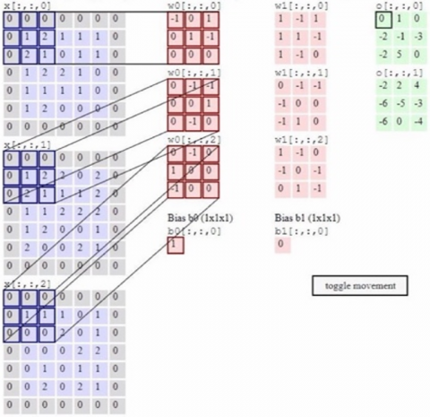
The convolution layer is an initial step in the CNN model, where convolution refers to the repetitive application of a function to the output of another function. Convolution operations involve the manipulation of two functions that take real values as arguments. At this stage, convolutions are applied to the output of the preceding layer using the convolutions operation [20]. This technique utilizes output functions as feature maps for the input image. The procedure of the convolutional layer is illustrated in Figure 2.
3.2.2 Activation layer
The activation layer function is utilized to ascertain the activation status of a neuron, which is contingent upon the magnitude of input weights. Deep learning typically utilizes several activation functions such as Tanh, ReLU, algebraic sigmoid, Leakly ReLU/PReLU, sigmoids, Randomized Leakli ReLu, Exponential Linear, and ReLU noisy units [17]. The activation layer utilized in this study is the Rectified Linear Unit (ReLU) function. The ReLU activation function can be observed in Figure 3.
Figure 1. CNN architectural planning
Figure 2. The procedure of the convolutional layer
Figure 3. ReLU activation
3.2.3 Pooling layer
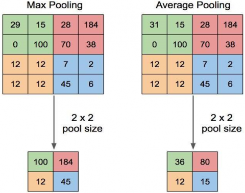
The pooling layer is positioned subsequent to the convolution layer. The layer comprises a filter and a stride of a specific magnitude, which are thereafter applied in an alternating manner throughout the pixel region of the feature map. This study will employ the technique of max pooling. The outcome of the pooling procedure is a matrix that is shown in Figure 4.
Figure 4. Pooling procedure
3.3 Model testing
Model testing is an essential step in assessing the performance of the developed CNN algorithm. The testing phase involves evaluating a model during its training stage. In this phase, the models are tested using diverse images to evaluate their accuracy in image classification. Currently, coffee seed classification involves making parameter adjustments to achieve the best possible outcomes. Parameter change refers to modifications in the data scenario and the number of epochs. This study examines three different data scenarios: (0.7:0.2:0.1), (0.8:0.1:0.1), and (0.6:0.3:0.1). Additional model testing is performed to compare the accuracy of each model and identify the model that exhibits the highest level of precision stability. The Eq. (1) describes the calculation used to determine the accuracy of the model.
Accuracy $=\frac{\Sigma \text { Prediction is True }}{\Sigma \text { data }}$ (1)
4.1 Model testing
This study utilizes a total of 360 datasets, with an equal distribution of 120 datasets in each class. The initial step involves organizing the dataset by uploading it to Google Drive. The dataset should be divided into three folders based on their respective classes: dark, green, light, and medium. The subsequent procedure involves partitioning three folders containing distinct data scripts into ratios of 70:30, 80:20, and 90:10. The splitfolder function will be used in the prose to implement this division. The data will be divided into a new folder named "data_classification_seed_copy_1" according to the specified ratio provided in the input. After performing the split, a new directory will be created, consisting of two subdirectories named "train" and "val". These subdirectories contain datasets with predetermined ratios. The subsequent phase involves employing data augmentation techniques to ensure that the computer can accurately detect a variety of images during the training process.
The data augmentation process is applied to the training data, which involves rescaling to 1/255, horizontal flipping, rotation with a scale of 40, width shifting, height shifting, shearing, and zooming with a scale of 0.2. The data source for the train_dir variable is determined during the augmentation process. The data used for analysis is sourced from the data_classification_biji_copy_1 dataset. The variable batch_size represents the number of images that are inserted during each step of the training process, which is set to 15 images. The color_mode variable represents the color filter applied to the RGB color model. The variable "class_mod" is categorical. During the data training process, the shuffle variable is set to True, resulting in random selection.
The CNN architecture implementation involves five convolutional layers, each with filters of 16, 32, 64, and 128. The data source is defined prior to this implementation. The CNN architecture is employed during the training phase to achieve an optimal model. The input image is a customized photo of coffee beans with dimensions of 512px×512px and three-color channels: Red, Green, and Blue (RGB). In the initial convolution, a 3×3 kernel and 16 filters were utilized for the filtering process. Stride refers to a filter shift of 1 pixel in both the horizontal and vertical directions. Next, employ the Rectified Linear Unit (ReLU) activation function to assign a value of 0 to any negative pixel. Next, apply MaxPooling to the pool using a kernel size of 2 pixels by 2 pixels and a stride size of 1 pixel. Pooling is a downsampling technique that reduces the input size by selecting the maximum pixel value within a kernel shift. This results in a smaller matrix. The second conversion process is like the first conversion process, but it varies in terms of input and the quantity of filters used. This process utilizes the output of the initial convergence process as input, with a filter size of 32. The third conversion process closely resembles the first convention process, as it utilizes the outputs of the second convergency process as its inputs. A total of 64 filters are employed for filtering, resulting in an image output of the same dimensions. This is due to the absence of pooling in the third convolutional process. The fourth conversion procedure is like the first, with the only difference being the use of output from the sequential conversion layer process as input.
The dropout technique is a method used in neural networks where a random subset of neurons is selected and utilized during the learning process. The dropout rate employed in this technique is typically set at 0.5. The flatten process transforms a pixel, obtained through dropout, into a 1-dimensional vector or matrix. The process involves three fully connected layers, with output sizes of 128 and 512 pixels for two of the layers. The ReLu activation function is utilized in these layers. After constructing the Convolutional Neural Network (CNN) model, the next step is to compile it. A model will be prepared for training. Three variables are used in compiled models. The method employs the categorical_crossentropy loss function to calculate the loss value. This study employs three optimization techniques, specifically Adam, RMSprop, and Nadam, using a learning rate of 0.0001. This study employed accuracy as the primary metric for calculation. Upon completion of model compilation, the training process is initiated. Machine learning employs pre-existing convolutional neural network (CNN) algorithms to effectively preserve class patterns during training.
4.2 Testing the epoch parameter
An epoch refers to the completion of one full cycle of the training process in a neural network, where the entire dataset is passed through both the forward and backward passes. However, due to the requirement of processing the entire dataset, the duration to complete one epoch in this neural network is considerably long. The batch size refers to the number of data samples allocated to the neural network. In this study, a batch size of 15 was utilized.
Data scenarios consist of datasets that are partitioned into training data and validation data. This study utilized a total of 360 data points, with each class containing 120 data points. The data will be trained using three different data scenarios: 70:30, 80:20, and 90:10. Each scenario will be trained for 20, 30, and 50 epochs. Additionally, three different optimization algorithms will be used: Adam, RMSprop, and Nadam.
4.2.1 Data training using epoch 20
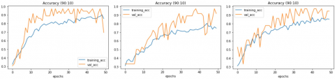
The training results, including epoch, data scenarios, and the use of optimization, were analyzed using graphical visualization on Google Colab. The objective was to determine whether the model is well-fitted, underfitted, or overfitted. Underfitting refers to a situation in which both the training accuracy and validation accuracy values are low, while the loss values are high. Overfitting is characterized by high training accuracy, low validation accuracy, and high loss values. A model is considered good or accurate when the orange and blue lines remain parallel, indicating high training accuracy and high validation values, while maintaining low losses.
Figure 5. Training and validation accuracy on epoch 20 data scenario 90:10
Table 1. Training results using epoch 20
|
Optimization |
Scenario (Training: Validation) |
Validation Accuracy |
Validation Loss |
|
Adam |
70:30 80:20 90:10 |
85.19% 79.17% 75.00% |
0.4063 0.6247 0.4570 |
|
RMSprop |
70:30 80:20 90:10 |
84.26% 79.17% 86.11% |
0.5360 0.4792 0.5010 |
|
Nadam |
70:30 80:20 90:10 |
88.89% 79.17% 83.33% |
0.4245 0.5092 0.3779 |
Figure 5 shows that the validation accuracy results on the optimization of Adam, the optimisation of RMSprop and the optimization of blemish are the same, i.e. 79.17%. On the model there are still fluctuating changes in the training accuracy as well as validation accuracy. On the third training data below are the results of validation accuracy with epoch 20 and the data scenario 90:10 as shown in Figure 5. The results of the entire training using the data of epoch 20 can be seen in Table 1.
Validation accuracy is obtained by testing the model using the validation of data derived from the split data set based on the data scenario and the use of its optimization. Based on Table 1, the highest validation accurate result is achieved with the optimization of the blur in the 70:30 scenario, which is 88.89%, but the best validation loss is in the 90:10 scenario of the data blur optimization which is 0.3779. It can also be seen on the optimization of the Adam by looking at the surface distance on the graph between the train data and the validation data is very good which potentially avoids underfitting even if the accuracy is still below the blur. Thus, it can be concluded that in epoch 20 with a scenario of 70:30 blur optimization is able to obtain the highest accuracy result and the best loss value, but in adam optimization here it is capable of producing the most stable graphics.
4.2.2 Data training using epoch 30
Figure 6 illustrates the validation loss outcomes for different optimization techniques. The smooth optimization approach achieved the most favorable result with a value of 0.1769. In comparison, the RMSprop optimization yielded a validation loss of 0.2354, while the Adam optimization exhibited the poorest performance with a validation loss of 0.2415. The model exhibits fluctuating changes in both training loss and validation losses. However, the optimization techniques of Adam and RMSProp appear to indicate underfitting. Table 2 displays the outcomes of the complete training data after 30 epochs.
Figure 6. Training and validation loss on epoch 30 data scenario 90:10
Table 2. Training results using epoch 30
|
Optimization |
Scenario (Training: Validation) |
Validation Accuracy |
Validation Loss |
|
Adam |
70:30 80:20 90:10 |
87.96% 77.78% 91.67% |
0.4250 0.6891 0.2415 |
|
RMSprop |
70:30 80:20 90:10 |
76.85% 56.94% 94.44% |
0.6140 0.9552 0.2354 |
|
Nadam |
70:30 80:20 90:10 |
67.59% 88.89% 97.22% |
0.7856 0.4163 0.1769 |
Table 2 shows that the best validation accuracy and validation loss results are obtained on smooth optimization with a scenario of 90:10, which is 97.22% validation accuracy and 0.1769 validation losses. Seeing from the graph on the smooth optimization in epoch 30 this looks better than the optimization of Adam or RMSprop, seen in the surface distance on the graph between data train and data validation more stable that minimizes the occurrence of over fitting or underfitting.
4.2.3 Data training using epoch 50
Figure 7 shows that the highest validation accuracy is 94.44%, then RMSprop optimization is 91.67% and the lowest optimization of Adam is 69.44%. Here is the validation loss result with epoch 50 and the 70:30 data scenario shown in Figure 6.
Figure 7. Training and validation loss on epoch 50 data scenario 70:30
Figure 7 illustrates the validation loss results for different optimization methods. The Adam optimization achieved the best result with a loss of 0.3094, followed by RMSprop with a loss of 0.5145. The least effective optimization method was observed to be 0.7041. The model exhibits ongoing fluctuations in the validation loss. Figure 7 displays the validation loss for epoch 50 in the 80:20 data scenario. The results of the entire training data using epoch 50 can be seen in Table 3.
Table 3. Training results using epoch 50
|
Optimization |
Scenario (Training: Validation) |
Validation Accuracy |
Validation Loss |
|
Adam |
70:30 80:20 90:10 |
91.67% 70.83% 69.44% |
0.3094 0.6926 0.7777 |
|
RMSprop |
70:30 80:20 90:10 |
81.48% 94.44% 91.67% |
0.6140 0.9552 0.2354 |
|
Nadam |
70:30 80:20 90:10 |
71.30% 79.30% 94.44% |
0.7041 0.5691 0.2053 |
Table 3 demonstrates that the optimal validation accuracy and validation loss outcomes are achieved through smooth optimization with a 90:10 scenario, yielding a validation accuracy of 94.44% and a validation loss of 0.2053. At epoch 50, there is a noticeable fluctuation in the surface distance between the training and validation data on the graph. This indicates a potential issue of overfitting or underfitting, despite the higher accuracy and decreasing loss value. The model's training results alone cannot determine the best model in this research. To assess the accuracy of the optimal model, researchers must also conduct testing using new data, in addition to the data used for training and validation.
4.3 Compare optimization model
The testing process aimed to assess the accuracy of the model by utilizing a set of 60 images, with 20 images representing each class. The results of model testing using data scenarios are presented in the following confusion matrix. The test results were obtained by utilizing epoch 30 on a data scenario with a 80:20 split.
Table 4 demonstrates that while utilizing 60 new photos in each optimization and epoch 30 in the 80:20 data scenario, the model achieved proper testing data for 49 images in the optimization, 46 images with RMSprop optimization, and 42 images with blur optimization.
Table 4. Confusion matrix using epoch 30, data scenario 80:20
|
Optimization |
Confusion Matrix |
Prediction Class |
|||
|
Dark |
Ripe |
Over Ripe |
|||
|
Adam |
Real Class |
Dark |
16 |
1 |
3 |
|
Ripe |
5 |
18 |
2 |
||
|
Over ripe |
0 |
0 |
20 |
||
|
RMSprop |
Real Class |
Dark |
11 |
8 |
1 |
|
Ripe |
2 |
17 |
1 |
||
|
Over ripe |
0 |
4 |
16 |
||
|
Nadam |
Real Class |
Dark |
16 |
2 |
2 |
|
Ripe |
5 |
12 |
3 |
||
|
Over ripe |
6 |
0 |
14 |
||
Table 5. Test results for all models
|
Optimization |
Epoch |
Scenario Data |
Accuracy |
|
Adam |
20 20 20 30 30 30 50 50 50 |
70:30 80:20 90:10 70:30 80:20 90:10 70:30 80:20 90:10 |
75.00% 75.00% 58.33% 80.00% 81.67% 76.67% 73.33% 63.33% 56.67% |
|
RMSprop |
20 20 20 30 30 30 50 50 50 |
70:30 80:20 90:10 70:30 80:20 90:10 70:30 80:20 90:10 |
75.00% 56.67% 78.33% 78.33% 76.67% 63.33% 55.00% 66.67% 60.00% |
|
Nadam |
20 20 20 30 30 30 50 50 50 |
70:30 80:20 90:10 70:30 80:20 90:10 70:30 80:20 90:10 |
71.67% 55.00% 70.00% 58.33% 70.00% 75.00% 65.00% 60.00% 58.33% |
The third test of the optimization technique yielded the following results, as shown in Table 5: The Adam optimizer has exceptional performance in the early epochs (20) for both the 70:30 and 80:20 data scenarios, with an accuracy of 75% in both instances. Nevertheless, as the ratio of testing data climbs to 90:10, there is a notable decline in accuracy. When the number of epochs is increased to 30, the accuracy improves for the 70:30 and 80:20 situations. However, there is a drop in accuracy when the number of epochs is further increased to 50. The RMSprop optimizer consistently achieves high performance when trained for 20 and 30 epochs, using a data split scenario of 70:30 and 80:20. During epoch 20, this optimizer gets the highest accuracy of 78.33% in the 90:10 scenario. The correlation between the increase in the number of epochs and the improvement in accuracy seems to be inconsistent. The Nadam optimizer algorithm has varied outcomes, achieving a peak accuracy of 75% after 30 epochs in a data situation where the training and testing data are split in a 90:10 ratio. Like RMSprop, the accuracy diminishes as the number of epochs increases for the 70:30 and 80:20 data scenarios, suggesting that more epochs do not always lead to better performance.
Based on testing result the model that achieves the highest accuracy when using new data is the one that utilizes the optimization technique called Adam at epoch 30 and the data scenario 80:20. This model achieves an accuracy of 81.67%. Across all situations, there is a consistent trend of diminishing accuracy as the proportion of test data increases. This indicates the significance of acquiring a larger amount of training data to achieve more precise models. Moreover, the inclusion of epoch numbers does not necessarily correlate with a rise in accuracy. To enhance future study, it would be advantageous to explore the fundamental elements that contribute to the diverse levels of precision among different optimization strategies and data circumstances. Additional research could investigate the influence of supplementary hyperparameters, such as learning rates or batch sizes, on the performance of the model.
This research project was completed with the generous support of an internal grant from Universitas Jember, provided under the University's Visionary Support Grant Scheme (Grant No.: 3780/UN25.3.1/LT/2023). We would like to extend our sincere appreciation to Universitas Jember for their generous support in terms of funding and resources, which have been instrumental in facilitating the successful execution of this research project. This research aligns with the university's vision and mission, aiming to contribute to knowledge advancement. The financial support from Universitas Jember has been instrumental in facilitating the research process, encompassing data collection, analysis, and dissemination of findings.
[1] Wang, Y.F., Cheng, C.C., Tsai, J.K. (2022). Implementation of green coffee bean quality classification using slim-CNN in Edge computing. In 2022 IEEE 5th International Conference on Knowledge Innovation and Invention (ICKII), Hualien, Taiwan, pp. 133-135. https://doi.org/10.1109/ICKII55100.2022.9983596
[2] Febriana, A., Muchtar, K., Dawood, R., Lin, C.Y. (2022). USK-COFFEE dataset: A multi-class green Arabica coffee bean dataset for deep learning. In 2022 IEEE International Conference on Cybernetics and Computational Intelligence (CyberneticsCom), Malang, Indonesia, pp. 469-473. https://doi.org/10.1109/CyberneticsCom55287.2022.9865489
[3] Huang, N.F., Chou, D.L., Lee, C.A. (2019). Real-time classification of green coffee beans by using a convolutional neural network. In 2019 3rd International Conference on Imaging, Signal Processing and Communication (ICISPC), Singapore, pp. 107-111. https://doi.org/10.1109/ICISPC.2019.8935644
[4] Pinto, C., Furukawa, J., Fukai, H., Tamura, S. (2017). Classification of Green coffee bean images basec on defect types using convolutional neural network (CNN). In 2017 International Conference on Advanced Informatics, Concepts, Theory, and Applications (ICAICTA), Denpasar, Indonesia, pp. 1-5. https://doi.org/10.1109/ICAICTA.2017.8090980
[5] Sánchez-Aguiar, A.F., Ceballos-Arroyo, A.M., Espinosa-Bedoya, A. (2019). Toward the recognition of non-defective coffee beans by means of digital image processing. In 2019 XXII Symposium on Image, Signal Processing and Artificial Vision (STSIVA), Bucaramanga, Colombia, pp. 1-5. https://doi.org/10.1109/STSIVA.2019.8730267
[6] Ramirez-Ticona, J., Gutiérrez-Cáceres, J.C., Portugal-Zambrano, C.E. (2016). Cell-phone based model for the automatic classification of coffee beans defects using white patch. In 2016 XLII Latin American Computing Conference (CLEI), Valparaiso, Chile, pp. 1-6. https://doi.org/10.1109/CLEI.2016.7833335
[7] Triyanto, W.A., Adi, K., Suseno, J.E. (2024). Indoor location mapping of lameness chickens with multi cameras and perspective transform using convolutional neural networks. Mathematical Modelling of Engineering Problems, 11(2): 539-548. https://doi.org/10.18280/mmep.110227
[8] Zhang, C., Sargent, I., Pan, X., Gardiner, A., Hare, J., Atkinson, P.M. (2018). VPRS-based regional decision fusion of CNN and MRF classifications for very fine resolution remotely sensed images. IEEE Transactions on Geoscience and Remote Sensing, 56(8): 4507-4521. https://doi.org/10.1109/TGRS.2018.2822783
[9] Peryanto, A., Yudhana, A., Umar, R. (2020). Klasifikasi citra menggunakan convolutional neural network dan K fold cross validation. Journal of Applied Informatics and Computing, 4(1): 45-51. https://doi.org/10.30871/jaic.v4i1.2017
[10] Portugal-Zambrano, C.E., Gutiérrez-Cáceres, J.C., Ramirez-Ticona, J., Beltran-Castañón, C.A. (2016). Computer vision grading system for physical quality evaluation of green coffee beans. In 2016 XLII Latin American Computing Conference (CLEI), Valparaiso, Chile, pp. 1-11. https://doi.org/10.1109/CLEI.2016.7833383
[11] Delenia, E., Putra, Y.H., Triwibowo, B.A., De La Croix, N.J., Ahmad, T. (2024). Detecting hidden data in images using Convolutional Neural Networks. Mathematical Modelling of Engineering Problems, 11(5): 1227-1235. https://doi.org/10.18280/mmep.110511
[12] Yanto, B., Fimawahib, L., Supriyanto, A., Hayadi, B.H., Pratama, R.R. (2021). Klasifikasi tekstur kematangan buah jeruk manis berdasarkan tingkat kecerahan warna dengan metode deep learning convolutional neural network. Jurnal Inovtek Polbeng Seri Informatika, 6(2): 259-268. https://doi.org/10.35314/isi.v6i2.2104
[13] Pratiwi, N.K.C., Ibrahim, N., Fu’adah, Y.N., Rizal, S. (2021). Deteksi parasit plasmodium pada citra mikroskopis hapusan darah dengan metode deep learning. ELKOMIKA: Jurnal Teknik Energi Elektrik, Teknik Telekomunikasi, & Teknik Elektronika, 9(2): 306. https://doi.org/10.26760/elkomika.v9i2.306
[14] LeCun, Y., Bengio, Y. (1995). Convolutional networks for images, speech, and time series. The Handbook of Brain Theory and Neural Networks, 3361(10): 1995.
[15] Hubel, D.H., Wiesel, T.N. (1968). Receptive fields and functional architecture of monkey striate cortex. The Journal of Physiology, 195(1): 215-243. https://doi.org/10.1113/jphysiol.1968.sp008455
[16] Farabet, C., Martini, B., Akselrod, P., Talay, S., LeCun, Y., Culurciello, E. (2010). Hardware accelerated convolutional neural networks for synthetic vision systems. In Proceedings of 2010 IEEE International Symposium on Circuits and Systems, Paris, France, pp. 257-260. https://doi.org/10.1109/ISCAS.2010.5537908
[17] Afaq, S., Rao, S. (2020). Significance of epochs on training a neural network. International Journal of Scientific and Technological Research, 9(06): 485-488.
[18] Lahouaoui, L., Abdelhak, D., Abderrahmane, B., Toufik, M. (2022). Image classification using a fully convolutional neural network CNN. Mathematical Modelling of Engineering Problems, 9(3): 771-778. https://doi.org/10.18280/mmep.090325
[19] Dong, J., Li, X. (2020). An image classification algorithm of financial instruments based on convolutional neural network. Traitement du Signal, 37(6): 1055-1060. https://doi.org/10.18280/ts.370618
[20] Jin, D., Xu, S., Tong, L., Wu, L., Liu, S. (2020). End image defect detection of float glass based on faster region-Based convolutional neural network. Traitement du Signal, 37(5): 807-813. https://doi.org/10.18280/ts.370513