R. Nithya![]() | K. Anitha*
| K. Anitha*![]()
© 2024 The authors. This article is published by IIETA and is licensed under the CC BY 4.0 license (http://creativecommons.org/licenses/by/4.0/).
OPEN ACCESS
This paper explores the effectiveness of different similarity measures for characterizing vertices and edges in rough graphs, which were introduced to handle imprecise and uncertain information. The authors examine traditional similarity measures like the Jaccard index, Dice coefficient, and overlap measure in this context. Additionally, a new ζ-labeling similarity measure for rough graphs is proposed. The main goal is to perform a comparative analysis evaluating the performance of these diverse similarity measures when applied to rough graphs. Furthermore, the paper computes the energy of rough graphs, defined as the sum of absolute eigenvalues, to demonstrate the superior potency of the proposed ζ-labeling measure compared to the other similarity measures considered. Overall, this work aims to advance techniques for assessing similarity in rough graphs, which have applications in dealing with vague and imprecise data.
rough membership value, rough graph, ζ-labeling similarity measure
Rough set theory, a prominent mathematical framework developed by Professor Pawlak to address uncertain problems, was extended to the domain of graphs through the work of Tong in 2006 [1], which leveraged approximations and led to varied forms of representations of rough graphs, including weighted rough graphs and directed rough graphs [2, 3]. Mathew et al. [4] established the notion of a vertex rough graph, delving into precision at both vertex and edge levels. Their investigation involved comparing two rough graphs using the degree of Similarity Measure. In this paper, we propose labeling through similarity measures for the graph from an Information system.
For managing imprecise data, Rough sets address boundary cases, while Fuzzy sets handle graded membership. These sets have found widespread application by researchers in both academic studies and practical, real-world situations [5-10]. The realm of classical and fuzzy graph labeling is discussed [7-12], encompasses diverse variations. While classical graph labeling techniques have been applied in areas like network analysis, data compression, optimization, image processing, and cryptography, the labeling of rough and fuzzy graphs caters to data involving partial truths and uncertain knowledge bases. Many researchers have investigated the concept of rough graphs through the lens of approximation methods. Anitha and Arunadevi for instance, devised a rough graph by assigning fixed rough membership values to objects within an Information System. Their work included the computation of the metric dimension of the rough graph [13].
After extensive research on rough graphs, Anitha and Nithya pioneered and explored a labeling technique, as labeling has emerged as a rapidly growing area of study across various fields. Their novel approach introduced the concept of ζ-graceful labeling applied to different representations of rough graphs [14].
In graph theory, graph energy represents a significant concept that captures the structural characteristics of a graph in a numerical form. It is defined as the trace of the graph's adjacency matrix. This notion of graph energy was originally proposed by Ivan Gutman, who demonstrated its applicability to certain families of graphs [15-18]. Extending this line of inquiry, Nagarani et al. explored the notion of energy within the context of fuzzy labeling graphs [19]. Alexander et al. made noteworthy contributions by addressing four conjectures related to path energy in graphs. They also devised an efficient algorithm for computing the path matrix [20], while Pirzada and Ganie introduced the Laplacian matrix derived from the adjacency matrix [21]. In this study, we further advance the understanding of energy within the domain of ζ-labeling rough graphs, underpinned by similarity measures.
Pappis and Karacapilidis [22] put forth the subsequent trio of similarity measures applicable to fuzzy sets as,
$\begin{gathered}M_{A, B}=\frac{\sum_i \min \left(a_i, b_i\right)}{\sum_i \max \left(a_i, b_i\right)} \\ L_{A, B}=1-\max _i\left(\left|a_i-b_i\right|\right) \\ S_{A, B}=1-\frac{\sum_i \min \left(a_i, b_i\right)}{\sum_i \max \left(a_i, b_i\right)}\end{gathered}$
Zadeh pioneered the concept of using similarity measures for fuzzy sets, which proved to be a successful strategy in handling uncertainty [23]. Simultaneously, similarity indexes emerged as a tool to gauge approximate equality among fuzzy sets within a specific universe of discourse. Following this, Wang [24] presented an overview of fuzzy set similarity measures and introduced two novel measures to quantify similarity between fuzzy sets and individual elements. Beyond Zadeh's groundwork in fuzzy set similarity measures, various researchers extended these notions to encompass multiple sets and vague sets [25-30]. In a parallel vein, other researchers ventured into the domain of similarity measures, tackling applications like text comparison using notions such as soft cardinality, similarity-based ranking, and query processing in multimedia databases and text mining. These authors proposed a novel similarity measure for fuzzy graphs, which seamlessly extends to the realm of fuzzy signatures, finding utility in analyzing workforce behavioral data. Furthermore, they generalized a similarity measure from trapezoidal fuzzy numbers to interval-valued trapezoidal fuzzy numbers, ensuring the preservation of its original properties [31, 32].
Extending previous similarity measures, we introduced a new similarity metric tailored to a novel labeling approach, which we explored for various representations of rough graphs constructed from high-dimensional data.
The primary aim of this paper is to propose a novel ζ-labeling similarity measure and evaluate its performance in comparison with existing similarity measures in the context of rough graphs. Additionally, this paper highlights the application of ζ-labeling similarity measures to rough graphs, with a focus on analyzing their energy. The synergy of rough ζ-labeling and the modified similarity measure yields the rough ζ-labeling similarity measure.
The paper commences with Section 2, which lays out the fundamental concepts of rough sets and rough graphs. Subsequently, Section 3 explores the notion of similarity relations in depth. Section 4 elucidates the methodology for labeling vertices and edges using similarity measures. Finally, the same section examines the connection between the energies of similarity measures, culminating in the concluding remarks presented in Section 5.
1.1 Exploring similarity measures
Similarity measures are mathematical techniques used to quantify the degree of similarity or dissimilarity between two objects, entities, or data points. They play a crucial role in various fields, including data analysis, pattern recognition, machine learning, and information retrieval. Similarity measures are used to compare objects based on their features or attributes and determine how closely they resemble each other.
There are several types of similarity measures and they can be broadly categorized into the following:
(a) Jaccard similarity coefficient
The Jaccard coefficient, also referred to as the Jaccard similarity coefficient or Jaccard index, is a metric used to quantify the similarity between two sets. It is defined as the size of the intersection of the sets divided by the size of their union. Mathematically, the Jaccard coefficient (J) is calculated using the following formula:
$J(A, B)=\frac{|A \cap B|}{|A \cup B|}$
where, A and B are two sets to measure similarity. The Jaccard coefficient produces a value between 0 and 1. A value of 0 signifies that there is no similarity or common elements between the sets, while a value of 1 signifies complete similarity, indicating that the sets are identical.
(b) Dice similarity measure
The Dice coefficient is an alternative method for gauging the similarity between two sets. Its calculation employs the subsequent formula:
$\operatorname{Dice}(A, B)=\frac{2|A \cap B|}{|A|+|B|}$
The Dice coefficient furnishes an output ranging between 0 and 1. A value of 0 denotes the absence of overlap or similarity amid the sets, while a value of 1 signifies an impeccable overlap or total similarity. A heightened Dice coefficient implies a superior overlap or concordance between the segmented regions and the established ground truth.
(c) Overlap coefficient similarity measure
The Overlap coefficient measures the similarity between two sets by expressing the fraction of their overlap. It's alternatively referred to as the Overlap index or Overlap coefficient of Tversky. The calculation of the overlap coefficient involves the use of the following formula:
$\operatorname{Overlap}(A, B)=\frac{|A \cap B|}{\min (|A|,|B|)}$
The outcome of the overlap coefficient ranges between 0 and 1. A value of 0 denotes the absence of overlap or similarity between the sets, while a value of 1 signifies full overlap or complete similarity.
This section covers fundamental concepts related to Rough sets and Rough graphs.
2.1 Information system
Let $\mathcal{U}$ be a non-empty finite set, referred to as the universe of discourse, and $\mathcal{A}$ be a set of attributes. An information system $I_s$ is defined as a pair $(\mathcal{U}, \mathcal{A})$, where for every $k \in \mathcal{A}$, there exists a function $k: \mathcal{U} \rightarrow \mathscr{V}_k$, with $\mathscr{V}_k$ being the value set of attribute a. If there exists a decision attribute $ ԃ \notin \mathcal{A}$, called the decision attribute, and the elements of $\mathrm{A}$ are termed condition attributes, then the triplet $(\mathcal{U}, \mathcal{A}, ԃ) $ is called a decision system.
2.2 Rough membership function $\left(R M_f\right)$
The $R M_f$ value provides a way to represent and handle the uncertainty and imprecision associated with the membership of elements in a rough set, allowing for a more flexible and realistic representation of real-world data. $R M_f$ is characterized by $\varphi_{\mathcal{R}}: \mathfrak{T} \rightarrow[0,1]$ and defined by
$\omega_{\mathfrak{I}}^{\mathcal{R}}(y)=\frac{\left|[y]_{\mathcal{R}} \cap \mathfrak{I}\right|}{\left|[y]_{\mathcal{R}}\right|}, \forall y \in u$
2.3 Rough graph
Let $\mathcal{U}$ be a non-empty set called the universe, and let $\mathfrak{E}$ be a set of unordered pairs of distinct elements from $\mathcal{U}$. A graph $\mathbb{G}$ can be constructed from these elements with the following considerations:
An edge between two vertices in the graph exists if and only if the maximum of their associated membership values is greater than zero.
2.4 Energy measure of rough labeling graph
Definition 2.4.1 The matrix representing the rough labeling relation is coined as $M^{\varphi}=\left[m_{i j}^{\varphi}\right]$ where $m_{i j}^{\varphi}=\sigma^{\varphi}\left(v_i v_j\right)$.
Definition 2.4.3 The sum of the absolute values of the eigenvalues of the rough labeling matrix is known as the Energy of the rough graph $\mathcal{R}_{\mathcal{L}}^{\varphi}$ which is denoted by $\mathfrak{E}\left(\mathcal{R}_{\mathcal{L}}^{\varphi}\right)=$ $\sum_{i=1}^n\left|\Psi_i\right|$ and also it should satisfies the following criteria:
$\mathfrak{E}\left(\mathcal{R}_{\mathcal{L}}^{\varphi}\right)=\sum_{i=1}^n\left|\psi_i\right|$
$0 \leq \omega\left(v_i\right) \leq 1$
If $\mathcal{R}_{\mathcal{L}}^{\varphi}=\max \left(\omega\left(v_i^{\varphi}\right), \omega\left(v_j^{\varphi}\right)\right)>0$ then edge exists for $v_i, v_j \in V$.
Let $\mathbb{S}: \mathcal{R}_{\mathcal{L}}^{\varphi}\left(v_i, v_j\right) \rightarrow[0,1]$ be a function mapping pairs of elements from the universe $\mathcal{U}$ to the closed interval $[0,1]$. Then, $\mathbb{S}$ is said to be a similarity measure between $v_i, v_j$ in $\mathcal{U}$ if $\mathbb{S}$ satisfies the following properties:
3.1 Characteristics of similarity metric
Theorem 3.1.1 $S\left(v_i, v_j\right)=1$ iff $\left[v_i\right]_{\mathcal{S}_r}=\left[v_j\right]_{\mathcal{S}_r}$
Proof: $S\left(v_i, v_j\right)=1$ iff $S\left(\left[v_i\right]_{\mathcal{S}_r},\left|v_j\right|_{\mathcal{S}_r}\right)=1$ which is equivalent to $\left[v_i\right]_{\mathcal{S}_r}=\left[v_j\right]_{\mathcal{S}_r}$ taking into account the property $\left[v_i\right]_{\mathcal{S}_r} \subseteq X$ and $\left[v_j\right]_{\mathcal{S}_r} \subseteq X \Leftrightarrow \omega_X^R\left(v_i\right)=1$ and $\omega_X^R\left(v_j\right)=$ 1. So $S\left(v_i, v_j\right)=1$ where $v_i, v_j \in V$.
Theorem 3.1.2 $S\left(v_i, v_j\right)=0$ iff $\left[v_i\right]_{\mathcal{S}_r} \neq\left[v_j\right]_{\mathcal{S}_r}$
Proof: $S\left(v_i, v_j\right)=0$ iff $S\left(\left[v_i\right]_{\delta_r},\left[v_j\right]_{\mathcal{S}_r}\right)=0$ which is equivalent to $\left[v_i\right]_{\mathcal{S}_r} \cap X=0$ iff $\omega_X^R\left(v_i\right)=0$ and $\left[v_j\right]_{\mathcal{S}_r} \cap X=$ 0 iff $\omega_X^R\left(v_j\right)=0$.
Theorem 3.1.3 $0 \leq S\left(v_i, v_j\right) \leq 1$
Proof: For $X \subset U,\left[v_i\right]_{\delta_r} \subseteq X$ and $\left[v_j\right]_{S_r} \subseteq X$ where $v_i, v_j \in V$. Then $\left[v_i\right]_{\delta_r} \subseteq X$ iff $\left[v_j\right]_{\delta_r} \cap X \neq \emptyset$ iff $\omega_X^R\left(v_i\right)>$ 0 and $\left[v_j\right]_{\mathcal{S}_r} \subseteq X$ iff $\left[v_j\right]_{\mathcal{S}_r} \cap U-X \neq \emptyset$ iff $\omega_X^R\left(v_j\right)<1$. So, $0 \leq \omega_X^R\left(v_i\right) \leq 1 \quad$ and $\quad 0 \leq \omega_X^R\left(v_j\right) \leq 1 \quad, \quad 0 \leq$ $\max \left(\omega_X^R\left(v_i\right), \omega_X^R\left(v_j\right)\right) \leq 1$
Hence, we proved that $0 \leq S\left(v_i, v_j\right) \leq 1$.
Theorem 3.1.4 $S\left(v_i, v_j\right)=S\left(v_j, v_i\right)$
Proof: i) $S\left(v_i, v_j\right)=1$ iff $S\left(\left[v_i\right]_{s_r},\left[v_j\right]_{S_r}\right)=1$ which is equivalent to $\left[v_i\right]_{S_r}=\left[v_j\right]_{S_r}$ iff $\omega_X^R\left(v_i\right)=1$ and $\omega_X^R\left(v_j\right)=1$.
ii) $S\left(v_j, v_i\right)=1 \quad$ iff $S\left(\left[v_j\right]_{S_r},\left[v_i\right]_{\delta_r}\right)=1$ which is equivalent to $\left[v_j\right]_{S_r}=\left[v_i\right]_{S_r}$ iff $\omega_X^R\left(v_j\right)=1$ and $\omega_X^R\left(v_i\right)=1$.
From (i) and (ii) $\Rightarrow S\left(v_i, v_j\right)=S\left(v_j, v_i\right)$
Theorem 3.1.5 $\operatorname{Sim}\left(v_i, v_k\right) \leq \operatorname{Sim}\left(v_i, v_j\right) \quad$ and $\operatorname{Sim}\left(v_i, v_k\right) \leq \operatorname{Sim}\left(v_j, v_k\right)$
Proof: For any $v_i, v_j, v_k \in \mathcal{R}_{\mathcal{L}}^{\varphi}$,
$S\left(v_i, v_j\right)=1$ if $S\left(\left[v_i\right]_{S_r},\left[v_j\right]_{\mathcal{S}_r}\right)=1$ which is equivalent to $\left[v_i\right]_{\mathcal{S}_r}=\left[v_j\right]_{\mathcal{S}_r}$ if $\omega_X^R\left(v_i\right)=1$ and $\omega_X^R\left(v_j\right)=1$
And $S\left(v_j, v_k\right)=1 \Leftrightarrow S\left(\left[v_j\right]_{\mathcal{S}_r},\left[v_k\right]_{\mathcal{S}_r}\right)=1$ which is equivalent to $\left[v_j\right]_{\mathcal{S}_r}=\left[v_k\right]_{\mathcal{S}_r}$ iff $\omega_X^R\left(v_j\right)=1$ and $\omega_X^R\left(v_k\right)=$ 1. Therefore, it is proved that $S\left(v_i, v_k\right) \leq S\left(v_i, v_j\right)$. Similarly, $S\left(v_i, v_k\right) \leq S\left(v_j, v_k\right)$
3.2 Operations of similarity measures
1. Let $v_i$ is a subset of $v_j$ (i.e) $v_i \subseteq v_j$ iff $\left[v_i\right]_{\mathcal{S}_r} \subseteq$ $\left[v_j\right]_{S_r} \forall v_i, v_j \in V$.
2. Let $v_i$ is equal to $v_j$ (i.e.) $v_i=v_j \operatorname{iff}\left[v_i\right]_{\mathcal{S}_r} \subseteq\left[v_j\right]_{\mathcal{S}_r}$ and $\left[v_j\right]_{\mathcal{S}_r} \subseteq\left[v_i\right]_{\mathcal{S}_r}$, (i.e) iff $\left[v_i\right]_{\mathcal{S}_r}=\left[v_j\right]_{\mathcal{S}_r} \forall v_i, v_j \in V$.
3. The union of $v_i$ and $v_j$ is denoted by $\mathcal{S}_r\left(v_i \cup v_j\right)$ whose similarity classes are defined as $\mathcal{S}_r\left(v_i \cup v_j\right)=\left[v_j\right]_{\mathcal{S}_r} \vee\left[v_i\right]_{\mathcal{S}_r}$.
4. The intersection of $v_i$ and $v_j$ is denoted by $\mathcal{S}_r\left(v_i \cap v_j\right)$ whose similarity classes are defined as $\mathcal{S}_r\left(v_i \cup v_j\right)=\left[v_j\right]_{\mathcal{S}_r} \wedge$ $\left[v_i\right]_{\mathcal{S}_r}$.
5. The complement of $v_i$ is denoted as $\bar{v}_l$ whose similarity classes for each $v_i \in V$ where the vertices $v_i * v_j \in V$.
The combination of $\zeta-$ labeling formula and similarity measure in rough graph is termed as rough $\zeta$ - labeling similarity graph.
4.1 Rough ζ-labeling similarity graph
A rough graph $\mathcal{R}_{\mathcal{L}}^{\varphi}=\left(V, E, \rho^{\varphi}, \sigma^{\varphi}, \omega\right)$ is said to be rough $\zeta$ -Labeling Similarity Graph if $\mathrm{V}=\left\{\rho^{\varphi}\left(v_i\right)\right\}$ for $i=1,2, \ldots, n$ and $\mathrm{E}=\left\{\sigma^{\varphi}\left(v_i, v_j\right)\right\}$ for $i=1,2, \ldots, n$ and $\omega: V * V \rightarrow[0,1]$ is bijection such that edges and vertices can be labeled using similarity classes and measures if it satisfies the following requirements:
i. If $\mathcal{R}_{\mathcal{L}}^{\varphi}=\max \left(\omega\left(v_i^{\varphi}\right), \omega\left(v_j^{\varphi}\right)\right)>0$ then edge exists for $v_i, v_j \in V$.
ii. Vertex labeling: $\rho^{\varphi}\left(v_i\right)=\frac{\left[v_i\right] \delta_r}{n}$, where $\left[v_i\right]_{\mathcal{S}_r}=\left\{v_j /\right.$ $\left.v_i \mathcal{S}_r v_j\right\}$
iii. Edge labeling: $\sigma^{\varphi}\left(v_i, v_j\right)=\operatorname{Sim}_\zeta\left(v_i, v_j\right)=\frac{\zeta}{\zeta+\eta}$, where $\eta=\frac{\left|\left[v_i\right] s_r\right| *\left|\left[v_j\right]_{S_r}\right|}{\left|\left[v_i\right]_{\delta_r}\right|+\left|\left[v_j\right]_{\delta_r}\right|}$ and $\zeta=\rho^{\varphi}\left(v_i\right)+\rho^{\varphi}\left(v_j\right)+m$,
where, $\rho^{\varphi}\left(v_i\right)$ represents vertex labeling of $v_i, \rho^{\varphi}\left(v_j\right)$ represents the vertex labeling of $v_j, m$ represents the total no. of edges in rough graph.
Here ζ gives a labeling formula and $\eta$ mentions modified similarity measure based on similarity class.
When considering two similarity classes of objects, u and v, the computation of similarity measures is performed using Eqs. (1)-(4).
$\operatorname{Sim}_{\text {jaccard }}\left(v_i, v_j\right)=\operatorname{Sim}_j\left(v_i, v_j\right)=\frac{\left|\left[v_i\right]_{\mathcal{S}_r} \cap\left[v_j\right]_{\mathcal{S}_r}\right|}{\left|\left[v_i\right]_{\mathcal{S}_r} \cup\left[v_j\right]_{\mathcal{S}_r}\right|}$ (1)
$\operatorname{Sim}_{\text {dice }}\left(v_i, v_j\right)=\operatorname{Sim}_d\left(v_i, v_j\right)=\frac{2\left|\left[v_i\right]_{\mathcal{S}_r} \cap\left[v_j\right]_{\mathcal{S}_r}\right|}{\left|\left[v_i\right]_{S_r}\right|+\left|\left[v_j\right]_{\mathcal{S}_r}\right|}$ (2)
$\begin{aligned} & \operatorname{Sim}_{\text {min-overlap }}\left(v_i, v_j\right)=\operatorname{Sim}_O\left(v_i, v_j\right) =\min \left(\frac{\left|\left[v_i\right]_{\mathcal{S}_r} \cap\left[v_j\right]_{\mathcal{S}_r}\right|}{\left|\left[v_i\right]_{\mathcal{S}_r}\right|}, \frac{\left|\left[v_i\right]_{\mathcal{S}_r} \cap\left[v_j\right]_{\mathcal{S}_r}\right|}{\left|\left[v_j\right]_{\mathcal{S}_r}\right|}\right)\end{aligned}$ (3)
$\operatorname{Sim}_{\zeta-\text { label }}\left(v_i, v_j\right)=\operatorname{Sim}_\zeta\left(v_i, v_j\right)=\frac{\zeta}{\zeta+\eta}$ (4)
where, $\eta=\frac{\left|\left[v_i\right] s_r\right| *\left|\left[v_j\right]_{s_r}\right|}{\left|\left[v_i\right] s_r\right|+\left[v_j\right]_{S_r} \mid}$ and $\zeta=\rho^{\varphi}\left(v_i\right)+\rho^{\varphi}\left(v_j\right)+m$
$\rho^{\varphi}\left(v_i\right)$ and $\rho^{\varphi}\left(v_j\right)$ represent the vertex labeling of $v_i, v_j$ and $m$ represents the total no. of edges in rough graph.
All these similarity measures yield values within the range of 0 to 1. A value of 0 signifies a complete mismatch between two clusters, while a value of 1 signifies that the two clusters are identical.
4.2 Algorithm for computing the energy of rough graphs
The following algorithm outlines the steps to compute the Energy measure of a rough graph by employing rough vertex and edge labeling techniques.
Construct the rough graph by assigning membership values to vertices and edges using a membership function.
Compute the similarity classes from the given information table or data.
Label the vertices using a vertex labeling formula based on the similarity classes.
Assign labels to the edges using edge labeling formulas for various similarity measures.
Represent the labeled rough graph with similarity measures in a diagrammatic form.
Construct the adjacency matrix for rough graph, incorporating the various similarity measures assigned to the edges.
Calculate the eigenvalues of the adjacency matrix for each similarity measure.
Compute the Energy of the rough graph for each similarity measure by summing the absolute values of the corresponding eigenvalues.
Illustrative Case 1: Machine quality data
Consider a dataset consisting of information about five machines, with attributes: operation efficiency, number of machines, machine capacity, and a decision attribute representing quality.
Table 1. Decision system of machine quality data
|
Machines |
Operation Efficiency |
No. of Machine |
Machine Capacity h/day |
Quality |
|
m1 |
Advanced |
35 |
20 |
Good |
|
m2 |
Advanced |
29 |
12 |
Good |
|
m3 |
Advanced |
35 |
12 |
Good |
|
m4 |
Moderate |
18 |
15 |
Poor |
|
m5 |
Low |
35 |
20 |
Poor |
$\begin{gathered}\mathrm{R}\left\{m_1\right\}=\left\{m_1\right\}, \mathrm{R}\left\{m_2\right\}=\left\{m_2\right\}, \\ \mathrm{R}\left\{m_3\right\}=\left\{m_3\right\}, \mathrm{R}\left\{m_4\right\}=\left\{m_4\right\}, \mathrm{R}\left\{m_5\right\}=\left\{m_5\right\} .\end{gathered}$
Assuming that the outcome evaluation decision is good, we consider the target set as X={a, b}. Rough Membership values are
$\begin{aligned} & \omega\left(m_1\right)=\frac{\left|[x]_R \cap X\right|}{\left|[x]_R\right|}=1 ; \omega\left(m_2\right)=1 ; \omega\left(m_3\right)=0 \\ & \omega\left(m_4\right)=0 ; \omega\left(m_5\right)=0 \\ & \end{aligned}$
4.3 Similarity class
4.3.1 Calculation of similarity class
Based on the decision table (Table 1), we have constructed a similarity matrix that captures the relationships between objects with respect to their attributes. As there are three attributes in the dataset, each entry in Table 1 can take values from the set {0, 1, 2, 3}. The value 0 indicates that the two objects being compared have no overlapping attribute values, while a value of 3 signifies that the two objects are identical across all attributes.
From Table 2, the following similarity classes have been identified,
$\begin{gathered}{\left[m_1\right]_{\mathcal{S}_{\mathrm{r}}}=\{\mathrm{a}, \mathrm{b}, \mathrm{c}, \mathrm{e}\} ;\left|\left[m_1\right]_{\mathcal{S}_{\mathrm{r}}}\right|=4 ;\left[m_2\right]_{\mathcal{S}_{\mathrm{r}}}=\{\mathrm{a}, \mathrm{b}, \mathrm{c}\} ;\left|\left[m_2\right]_{\mathcal{S}_{\mathrm{r}}}\right|= 3;} \\\left[m_3\right]_{\mathcal{S}_{\mathrm{r}}}=\{\mathrm{a}, \mathrm{b}, \mathrm{c}, \mathrm{e}\} ;\left|\left[m_3\right]_{\mathcal{S}_{\mathrm{r}}}\right|=4 ;\left[m_4\right]_{\mathcal{S}_{\mathrm{r}}}=\{\mathrm{d}\} ;\left|\left[m_4\right]_{\mathcal{S}_{\mathrm{r}}}\right|=1;\\ \left[m_5\right]_{\mathcal{S}_{\mathrm{r}}}=\{\mathrm{a}, \mathrm{c}, \mathrm{e}\} ;\left|\left[m_5\right]_{\mathcal{S}_{\mathrm{r}}}\right|=3\end{gathered}$
Table 2. Similarity class of machine quality data
|
$\mathcal{S}_r$ |
m1 |
m2 |
m3 |
m4 |
m5 |
|
m1 |
0 |
0.75 |
1 |
0 |
0.75 |
|
m2 |
0 |
0 |
0.75 |
0 |
0.5 |
|
m3 |
1 |
0.75 |
0 |
0 |
0 |
|
m4 |
0 |
0 |
0 |
0 |
0 |
|
m5 |
0.75 |
0.5 |
0 |
0 |
0 |
4.4 Labeling methodology
$\rho^{\varphi}\left(v_i\right)=\frac{\left|\left[v_i\right]_{\mathcal{S}_r}\right|}{n}$
4.4.1 Vertex labeling
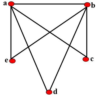
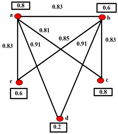
Figure 1 depicts the rough graph constructed from Table 1.
$\begin{gathered}\rho^{\varphi}(a)=0.8, \rho^{\varphi}(b)=0.6, \rho^{\varphi}(c)=0.8 \\ \rho^{\varphi}(d)=0.2, \rho^{\varphi}(e)=0.6\end{gathered}$.
Figure 1. Rough graph of machine quality data
4.4.2 Edge labeling
$E_G^{\varphi}\left(v_i, v_j\right)=\operatorname{Sim}\left(v_i, v_j\right) ; \operatorname{Sim}_\zeta\left(v_i, v_j\right)=\frac{\zeta}{\zeta+\eta}$
where, $\eta=\frac{\left|\left[v_i\right]_{\delta_r}\right| *\left|\left[v_j\right]_{\mathcal{S}_r}\right|}{\left|\left[v_i\right]_{\delta_r}\right|+\left|\left[v_j\right]_{\mathcal{S}_r}\right|}$ and $\zeta_{i j}=\rho^{\varphi}\left(v_i\right)+\rho^{\varphi}\left(v_j\right)+m$
Table 3 presents the edge labeling values assigned to the edges of the rough graph derived from the machine quality data.
Table 3. Edge labeling of rough graph
|
Edges |
$\zeta_{i j}$ |
$\boldsymbol{\eta}$ |
$\frac{\zeta}{\zeta+\eta}$ |
|
Sim(a,b) |
$\zeta_{a b}=8.4$ |
1.71 |
0.83 |
|
Sim(a,c) |
$\zeta_{a c}=8.6$ |
2 |
0.81 |
|
Sim(a,d) |
$\zeta_{a d}=8.0$ |
0.8 |
0.91 |
|
Sim(a,e) |
$\zeta_{a e}=8.4$ |
1.17 |
0.83 |
|
Sim(b,c) |
$\zeta_{bc}=8.4$ |
1.17 |
0.83 |
|
Sim(b,d) |
$\zeta_{a b}=7.8$ |
0.75 |
0.91 |
|
Sim(b,e) |
$\zeta_{be}=8.2$ |
1.5 |
0.85 |
4.5 Energy of rough graph using similarity measures
After assigning edge labels based on various similarity measures, such as Jaccard, Dice, Overlap, and ζ labeling, we construct the adjacency matrix for the rough graph. We then calculate the eigenvalues of the adjacency matrix. The Energy of the rough graph for each similarity measure is obtained by summing the absolute values of the corresponding eigenvalues.
4.5.1 Jaccord $\operatorname{Sim}_j\left(v_i, v_j\right)$
Here edges are labeled using Jaccord Similarity Measure as $\operatorname{Sim}_j\left(v_i, v_j\right)=\frac{\left|\left[v_i\right]_{\delta_r} \cap\left[v_j\right]_{\delta_r}\right|}{\left[\left[v_i\right]_{\delta_r} \cup\left[v_j\right]_{\delta_r} \mid\right.}$ and the adjacency matrix is given as shown in Table 4:
Table 4. Adjacency matrix for Figure 2
|
$\mathcal{S}_r$ |
m1 |
m2 |
m3 |
m4 |
m5 |
|
m1 |
3 |
1 |
2 |
0 |
2 |
|
m2 |
3 |
3 |
2 |
0 |
0 |
|
m3 |
2 |
2 |
3 |
0 |
1 |
|
m4 |
0 |
0 |
0 |
3 |
0 |
|
m5 |
2 |
0 |
1 |
0 |
3 |
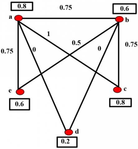
Figure 2 illustrates the vertex, edge labeling values assigned to the rough graph.
Figure 2. Jaccord similarity for Figure 1
Eigen values={0,-1.316,-0.383,0.005,1.695}
Energy of $\operatorname{Sim}_j\left(v_i, v_j\right)=3.399$
4.5.2 Dice $\operatorname{Sim}_d\left(v_i, v_j\right)$
Here, by using $Sim_d\left(v_i, v_j\right)=\frac{2\left|\left[v_i\right]_{S_r} \cap\left[v_j\right]_{\delta_r}\right|}{\left|\left[v_i\right]_{S_r}\right|+\left|\left[v_j\right]_{\delta_r}\right|}$, the edges are labeled and adjacency matrix is given as shown in Table 5:
Table 5. Adjacency matrix for Figure 3
|
$\mathcal{S}_r$ |
m1 |
m2 |
m3 |
m4 |
m5 |
|
m1 |
0 |
0.85 |
1 |
0 |
0.85 |
|
m2 |
0 |
0 |
0.85 |
0 |
0.66 |
|
m3 |
1 |
0.85 |
0 |
0 |
0 |
|
m4 |
0 |
0 |
0 |
0 |
0 |
|
m5 |
0.85 |
0.66 |
0 |
0 |
0 |
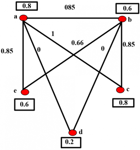
Figure 3. Labeling using Dice similarity for Figure 1
Eigen values = {0, -1.428, -0.451,0.003,1.876}
Energy = 3.758
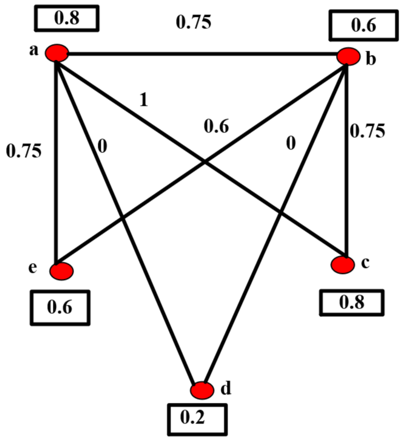
4.5.3 Overlap $\operatorname{Sim}_O\left(v_i, v_j\right)$
For overlap similarity measure $\operatorname{Sim}_O\left(v_i, v_j\right)=\min \left(\frac{\left|\left[v_i\right]_{s_r} \cap\left[v_j\right]_{s_r}\right|}{\left|\left[v_i\right]_{s_r}\right|}, \frac{\left|\left[v_i\right]_{s_r} \cap\left[v_j\right]_{S_r}\right|}{\left|\left[v_j\right]_{s_r}\right|}\right)$, the edges are labeled and its adjacency matrix is given in Table 6.
Table 6. Adjacency matrix for Figure 4
|
$\mathcal{S}_r$ |
m1 |
m2 |
m3 |
m4 |
m5 |
|
m1 |
0 |
0.75 |
1 |
0 |
0.75 |
|
m2 |
0 |
0 |
0.7 |
0 |
0.6 |
|
m3 |
1 |
0.75 |
0 |
0 |
0 |
|
m4 |
0 |
0 |
0 |
0 |
0 |
|
m5 |
0.75 |
0.6 |
0 |
0 |
0 |
Figure 4. Overlap similarity measures for Figure 1
Eigen values: {0, -1.348, -0.387, 0.002, 1.733}
Energy: 3.47
4.5.4 Rough $\zeta \operatorname{Sim}_\zeta\left(v_i, v_j\right)$
By implementing $\quad \operatorname{Sim}_\zeta\left(v_i, v_j\right)=\frac{\zeta}{\zeta+\eta} \quad$ where $\quad \eta=$ $\frac{\left|\left[v_i\right]_{\delta_r}\right| *\left[v_j\right]_{\delta_r} \mid}{\left|\left[v_i\right]_{\delta_r}\right|+\left|\left[v_j\right]_{\delta_r}\right|}$ and $\zeta=\rho^{\varphi}\left(v_i\right)+\rho^{\varphi}\left(v_j\right)+m$ (Table 7).
Table 7. Adjacency matrix for Figure 5
|
$\mathcal{S}_r$ |
m1 |
m2 |
m3 |
m4 |
m5 |
|
m1 |
0 |
0.83 |
0.81 |
0.9 |
0.83 |
|
m2 |
0.83 |
0 |
0.83 |
1 |
0.85 |
|
m3 |
0.81 |
0.83 |
0 |
0.9 |
0 |
|
m4 |
0.91 |
0.91 |
0 |
0 |
0 |
|
m5 |
0.83 |
0.85 |
0 |
0 |
0 |
Figure 5. Overlap similarity measure for Figure 1
Eigen values: {0,-1.726,-0.830,0,2.556}
Energy: 5.112
The following Table 8 presents a comparative analysis of the Energy values for the machine quality dataset, computed using different similarity measures such as Jaccard, Dice, Overlap, and the Rough ζ Similarity Measure.
Table 8. Comparative analysis of energy of similarity measures for rough graph 1
|
Edges |
Jaccard |
Dice |
Overlap |
ζ |
|
Sim(a, b) |
0.75 |
0.85 |
0.75 |
0.83 |
|
Sim(a, c) |
1 |
1 |
1 |
0.81 |
|
Sim(a, d) |
0 |
0 |
0 |
0.91 |
|
Sim(a, e) |
0.75 |
0.85 |
0.75 |
0.83 |
|
Sim(b, c) |
0.75 |
0.85 |
0.75 |
0.83 |
|
Sim(b, d) |
0 |
0 |
0 |
0.91 |
|
Sim(b, e) |
0.5 |
0.66 |
0.6 |
0.85 |
|
Energy |
3.399 |
3.758 |
3.47 |
5.112 |
Illustrative Case 2: In this case (Table 9), we have considered a dataset consisting of ten Iris flower samples, where the sepal length, sepal width, petal length, and petal width are treated as independent attributes or features. The decision attributes are the Iris species Setosa and versicolor.
Table 9. Iris flower data set
|
Iris Flower |
Sepal Length (cm) |
Sepal Width (cm) |
Petal Length (cm) |
Petal Width (cm) |
Iris Class |
|
f1 |
5 |
4 |
3 |
1 |
Setosa |
|
f2 |
4 |
9 |
3 |
1 |
Setosa |
|
f3 |
4 |
8 |
3 |
4 |
Setosa |
|
f4 |
5 |
5 |
2 |
4 |
Versicolor |
|
f5 |
5 |
6 |
2 |
9 |
Versicolor |
|
f6 |
5 |
6 |
3 |
0 |
Versicolor |
|
f7 |
5 |
7 |
4 |
4 |
Setosa |
|
f8 |
5 |
8 |
2 |
7 |
Versicolor |
|
f9 |
6 |
0 |
2 |
9 |
Versicolor |
|
f10 |
5 |
7 |
3 |
8 |
Setosa |
Let us consider the decision attribute as versicolor and the target set is X={ f4, f5, f6, f8, f9}.
Equivalence classes for Table 9:
$\mathrm{R}\left\{f_1\right\}=\left\{f_1\right\}, \mathrm{R}\left\{f_2\right\}=\left\{f_2\right\}, \mathrm{R}\left\{f_3\right\}=\left\{f_3\right\}, \mathrm{R}\left\{f_4\right\}=\left\{f_4\right\}$,
$\mathrm{R}\left\{f_5\right\}=\left\{f_5\right\}, \mathrm{R}\left\{f_6\right\}=\left\{f_6\right\}, \mathrm{R}\left\{f_7\right\}=\left\{f_7\right\}, \mathrm{R}\left\{f_8\right\}=\left\{f_8\right\}$,
$\mathrm{R}\left\{f_9\right\}=\left\{f_9\right\}, \mathrm{R}\left\{f_{10}\right\}=\left\{f_{10}\right\}$
Rough membership values are
$\begin{gathered}\omega\left(f_1\right)=0 ; \omega\left(f_2\right)=0 ; \omega\left(f_3\right)=0 ; \omega\left(f_4\right)=1 ; \\ \omega\left(f_5\right)=1 ; \omega\left(f_6\right)=1 ; \omega\left(f_7\right)=0 ; \omega\left(f_8\right)=1 ; \\ \omega\left(f_9\right)=1 ; \omega\left(f_{10}\right)=0\end{gathered}$
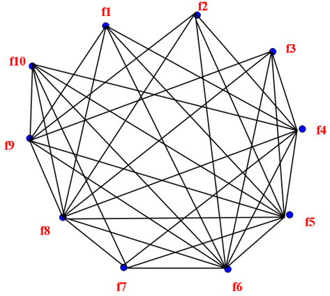
Figure 6. Rough graph of Iris flower data
Figure 6 illustrates the rough graph constructed based on the membership values assigned to each object in the dataset.
Table 10 presents the similarity classes derived from the rough graph shown in Figure 6, which was constructed based on the Iris flower dataset.
Table 10. Calculation of similarity class
|
$\mathcal{S}_r$ |
f1 |
f2 |
f3 |
f4 |
f5 |
f6 |
f7 |
f8 |
f9 |
f10 |
|
f1 |
4 |
2 |
1 |
1 |
1 |
2 |
1 |
1 |
0 |
2 |
|
f2 |
2 |
4 |
2 |
0 |
0 |
1 |
0 |
0 |
0 |
1 |
|
f3 |
1 |
2 |
4 |
1 |
0 |
1 |
1 |
1 |
0 |
1 |
|
f4 |
1 |
0 |
1 |
4 |
2 |
1 |
2 |
2 |
1 |
1 |
|
f5 |
1 |
0 |
0 |
2 |
4 |
2 |
1 |
2 |
2 |
1 |
|
f6 |
2 |
1 |
1 |
1 |
2 |
4 |
1 |
1 |
0 |
2 |
|
f7 |
1 |
0 |
1 |
2 |
1 |
1 |
4 |
1 |
0 |
2 |
|
f8 |
1 |
0 |
1 |
2 |
2 |
1 |
1 |
4 |
1 |
1 |
|
f9 |
0 |
0 |
0 |
1 |
2 |
0 |
0 |
1 |
4 |
0 |
|
f10 |
2 |
1 |
1 |
1 |
1 |
2 |
2 |
1 |
0 |
4 |
Vertex labeling: $\rho\left(f_1\right)=0.9 ; \rho\left(f_2\right)=0.5 ; \rho\left(f_3\right)=0.8; \begin{aligned} & \rho\left(f_4\right)=0.9 ; \rho\left(f_6\right)=0.9 ; \rho\left(f_7\right)=0.8 ; \rho\left(f_8\right)=0.9 ; \rho\left(f_9\right)=0.4 \text {; } \rho\left(f_{10}\right)=0.9\end{aligned}$.
Table 11 presents the edge labeling values for the rough graph constructed from the Iris flower dataset, computed using the Jaccard, Overlap, Dice, and Rough ζ similarity measures.
Table 11. Edge labels based on different similarity metrics
|
Edge Labeling |
Jaccord |
Dice |
Overlap |
ζ |
|
Sim (f1, f4) |
0.88 |
0.88 |
0.88 |
0.89 |
|
Sim (f1, f5) |
0.7 |
0.82 |
0.77 |
0.90 |
|
Sim (f1, f6) |
1 |
1 |
1 |
0.89 |
|
Sim (f1, f8) |
0.8 |
0.88 |
0.8 |
0.89 |
|
Sim (f1, f9) |
0.3 |
0.46 |
0.3 |
0.92 |
|
Sim (f2, f4) |
0.4 |
0.57 |
0.44 |
0.92 |
|
Sim (f2, f5) |
0.3 |
0.46 |
0.37 |
0.92 |
|
Sim (f2, f6) |
0.5 |
0.71 |
0.55 |
0.92 |
|
Sim (f2, f8) |
0.4 |
0.57 |
0.44 |
0.92 |
|
Sim (f2, f9) |
0 |
0 |
0 |
0.94 |
|
Sim (f3, f4) |
0.7 |
0.82 |
0.77 |
0.90 |
|
Sim (f3, f5) |
0.6 |
0.75 |
0.75 |
0.90 |
|
Sim (f3, f6) |
0.8 |
0.94 |
0.8 |
0.90 |
|
Sim (f3, f8) |
0.7 |
0.82 |
0.77 |
0.90 |
|
Sim (f3, f9) |
0.2 |
0.33 |
0.25 |
0.93 |
|
Sim (f4, f5) |
0.88 |
0.94 |
0.8 |
0.90 |
|
Sim (f4, f6) |
0.8 |
0.88 |
0.8 |
0.90 |
|
Sim (f4, f7) |
0.88 |
0.94 |
0.8 |
0.90 |
|
Sim (f4, f8) |
0.9 |
1 |
1 |
0.89 |
|
Sim (f4, f9) |
0.44 |
0.61 |
0.44 |
0.92 |
|
Sim (f4, f10) |
0.9 |
1 |
1 |
0.89 |
|
Sim (f5, f6) |
0.7 |
0.82 |
0.77 |
0.90 |
|
Sim (f5, f7) |
0.77 |
0.87 |
0.87 |
0.90 |
|
Sim (f5, f8) |
0.88 |
0.94 |
0.8 |
0.90 |
|
Sim (f5, f9) |
0.5 |
0.66 |
0.5 |
0.93 |
|
Sim (f5, f10) |
0.7 |
0.82 |
0.77 |
0.90 |
|
Sim (f6, f7) |
0.88 |
0.94 |
0.8 |
0.89 |
|
Sim (f6, f8) |
0.8 |
0.88 |
0.8 |
0.89 |
|
Sim (f6, f9) |
0.3 |
0.46 |
0.33 |
0.92 |
|
Sim (f6, f10) |
0.9 |
1 |
1 |
0.89 |
|
Sim (f7, f8) |
0.8 |
0.94 |
0.8 |
0.90 |
|
Sim (f7, f9) |
0.33 |
0.5 |
0.37 |
0.93 |
|
Sim (f8, f9) |
0.44 |
0.61 |
0.44 |
0.92 |
|
Sim (f8, f10) |
0.8 |
0.88 |
0.88 |
0.89 |
|
Sim (f9, f10) |
0.3 |
0.46 |
0.33 |
0.92 |
Table 12 presents the Energy values calculated for rough graph constructed from the Iris flower dataset, based on the adjacency matrix derived from the vertex and edge labeling using different similarity measures.
Table 12. Energy values of Iris flower rough graph
|
S. No |
Similarity Measure |
Energy Value |
|
1 |
Jaccord |
10.31 |
|
2 |
Dice |
10.41 |
|
3 |
Overlap |
11.69 |
|
4 |
ζ |
13.28 |
Illustrative Case 3: The dataset comprises information on six cast iron pipes (Table 13) subjected to a high-pressure endurance test. Let's designate the target set as $X=$ $\left\{P_1, P_5, P_6\right\}$. Rough membership values are as follows: $\omega\left(P_1\right)=0.5 ; \omega\left(P_2\right)=0 ; \omega\left(P_3\right)=0.5, \omega\left(P_4\right)=0 ; \omega\left(P_5\right)=$ $1, \omega\left(P_6\right)=1$.
Table 13. Iron pipes data
|
Iron Pipes |
Coal |
Sulfur |
Phosphorus |
Cracks |
|
P1 |
High |
High |
Low |
Yes |
|
P2 |
Average |
High |
Low |
No |
|
P3 |
High |
High |
Low |
Yes |
|
P4 |
Low |
Low |
Low |
No |
|
P5 |
Average |
Low |
High |
Yes |
|
P6 |
High |
Low |
High |
Yes |
Table 14. Energy values of iron pipes data
|
S. No |
Similarity Measure |
Energy Value |
|
1 |
Jaccord |
6.345 |
|
2 |
Dice |
7.626 |
|
3 |
Overlap |
7.294 |
|
4 |
ζ |
8.072 |
Table 14 presents the energy values computed using the Jaccard, Dice, Overlap, and ζ similarity measures for the given dataset.
Illustrative Case 4: The dataset comprises information on fifteen female patients who underwent multiple tests to assess their diabetic condition (Table 15).
Table 16 presents the Energy values computed using the Jaccard, Dice, Overlap, and ζ similarity measures for the female diabetic dataset.
Table 15. Female diabetic data
|
Patients |
Thirst |
Hunger |
Frequent |
Weight Loss |
Tiredness |
Diabetic |
|
w1 |
High |
High |
Low |
Low |
High |
High |
|
w2 |
High |
High |
Low |
Low |
Low |
High |
|
w3 |
High |
High |
High |
Low |
High |
High |
|
w4 |
High |
High |
High |
Low |
Low |
High |
|
w5 |
High |
Low |
High |
High |
High |
High |
|
w6 |
High |
High |
High |
High |
High |
High |
|
w7 |
High |
Low |
Low |
Low |
Low |
High |
|
w8 |
High |
High |
High |
High |
High |
High |
|
w9 |
High |
High |
Low |
Low |
High |
Low |
|
w10 |
High |
Low |
High |
Low |
High |
Low |
|
w11 |
High |
High |
High |
Low |
High |
Low |
|
w12 |
High |
Low |
Low |
Low |
Low |
Low |
|
w13 |
Low |
High |
Low |
High |
High |
Low |
|
w14 |
Low |
Low |
Low |
High |
Low |
Low |
|
w15 |
High |
High |
Low |
Low |
High |
Low |
Table 16. Energy values of female diabetic data
|
S. No |
Similarity Measure |
Energy Value |
|
1 |
Jaccord |
25.848 |
|
2 |
Dice |
26.137 |
|
3 |
Overlap |
25.848 |
|
4 |
ζ |
27.4285 |
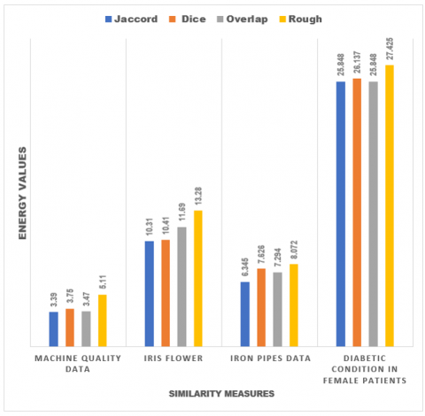
We have analyzed four distinct datasets, calculating energy values using Jaccard, Dice, Overlap, and Rough ζ measures. Across all four measures, Rough ζ consistently yields the highest energy values. Rough graph energy can provide insights into the structure and properties of complex networks, such as social networks, biological networks, and communication network. Figure 7 illustrates the graphical depiction of the comparative analysis.
Figure 7. Graphical depiction of comparative study
In this study, we conduct a comprehensive evaluation of various similarity measures for edge labeling in rough graphs. We present a unified view of these labeling similarity measures through the visualization of multiple bar charts. Additionally, we introduce a novel ζ labeling similarity metric designed to leverage similarity classes within rough graphs, utilizing its associated energy to characterize the graph's properties. This comprehensive overview of similarity metrics is facilitated through the representation of multiple bar charts. The energy of rough graphs can be exploited to identify significant nodes or links in a network, which has implications for network optimization, vulnerability analysis, and targeted interventions. This novel ζ labeling similarity metric, which capitalizes on similarity classes within rough graphs and quantifies the graph's characteristics through its energy, may find applications in cluster boundary region identification in Wireless Sensor Networks.
[1] Tong, H. (2006). Rough graph and its structure. Journal of Shandong University. https://en.cnki.com.cn/Article_en/CJFDTotal-SDDX200606010.htm.
[2] He, T., Chen, Y., Shi, K. (2006). Weighted rough graph and its application. In Sixth International Conference on Intelligent Systems Design and Applications, Jian, China, pp. 486-491. https://doi.org/10.1109/ISDA.2006.279
[3] He, T. (2012). Representation form of rough graph. Applied Mechanics and Materials, 157: 874-877. https://doi.org/10.4028/www.scientific.net/amm.157-158.874
[4] Mathew, B., John, S.J., Garg, H. (2020). Vertex rough graphs. Complex & Intelligent Systems, 6: 347-353. https://doi.org/10.1007/s40747-020-00133-8
[5] Pawlak, Z. (1991). Rough Sets: Theoretical Aspects of Reasoning about Data. http://bcpw.bg.pw.edu.pl/Content/1845/ZP_ksiazka.pdf.
[6] Anitha, K. (2014). Rough set theory on topological spaces. In Rough Sets and Knowledge Technology: 9th International Conference, RSKT 2014, Shanghai, China, pp. 69-74. https://doi.org/10.1007/978-3-319-11740-9_7
[7] Anitha, K., Venkatesan, P. (2016). Properties of hesitant fuzzy sets. Global Journal of Pure and Applied Mathematics (GJPAM), 12(1): 114-116.
[8] Kausar, N., Munir, M., Kousar, S., Gulistan, M., Anitha, K. (2020). Characterization of non-associative ordered semigroups by the properties of F-ideals. Fuzzy Information and Engineering, 12(4): 490-508. https://doi.org/10.1080/16168658.2021.1924513
[9] Anitha, K., Thangeswari, M. (2020). Rough set based optimization techniques. In 2020 6th International Conference on Advanced Computing and Communication Systems (ICACCS), Coimbatore, India, pp. 1021-1024. https://doi.org/10.1109/ICACCS48705.2020.9074212.
[10] Chen, J., Li, J. (2012). An application of rough sets to graph theory. Information Sciences, 201: 114-127. https://doi.org/10.1016/j.ins.2012.03.009
[11] Borzooei, R.A., Rashmanlou, H., Samanta, S., Pal, M. (2016). A study on fuzzy labeling graphs. Journal of Intelligent & Fuzzy Systems, 30(6): 3349-3355. https://doi.org/10.3233/ifs-152082
[12] Gani, A.N., Akram, M., Subahashini, D.R. (2014). Novel properties of fuzzy labeling graphs. Journal of Mathematics, 1-6. https://doi.org/10.1155/2014/375135
[13] Ramsankar, A.D., Krishnamoorthy, A. (2024). Exploring metric dimensions for dimensionality reduction and navigation in rough graphs. Mathematical Modelling of Engineering Problems, 11(4): 1037-1043. https://doi.org/10.18280/mmep.110421
[14] Nithya, R., Anitha, K. (2023). Even vertex ζ-graceful labeling on rough graph. Mathematics and Statistics, 11(1): 71-77. https://doi.org/10.13189/ms.2023.110108
[15] Gutman, I. (2001). The energy of a graph: Old and new results. In Algebraic Combinatorics and Applications: Proceedings of the Euro conference, Algebraic Combinatorics and Applications (ALCOMA), Gößweinstein, Germany, pp. 196-211. https://doi.org/10.1007/978-3-642-59448-9_13
[16] Li, X., Li, Y., Shi, Y., Gutman, I. (2012). Graph Energy. Springer, New York. https://doi.org/10.1007/978-1-4614-4220-2
[17] Gutman, I., Ramane, H.S. (2020). Research on graph energies in/2019. MATCH Communications in Mathematical and in Computer Chemistry, 84: 277-292.
[18] Nikiforov, V. (2007). The energy of graphs and matrices. Journal of Mathematical Analysis and Applications, 326(2): 1472-1475. https://doi.org/10.1016/j.jmaa.2006.03.072
[19] Nagarani, A., Vimala, S. (2017). Energy of fuzzy regular and graceful graphs. Asian Research Journal of Mathematics, 4(2): 1-8. https://doi.org/10.9734/arjom/2017/33057
[20] Ilić, A., Bašić, M. (2019). Path matrix and path energy of graphs. Applied Mathematics and Computation, 355: 537-541. https://doi.org/10.1016/j.amc.2019.03.002
[21] Pirzada, S., Ganie, H.A. (2015). On the Laplacian eigenvalues of a graph and Laplacian energy. Linear Algebra and its Applications, 486: 454-468. https://doi.org/10.1016/j.laa.2015.08.032
[22] Pappis, C.P., Karacapilidis, N.I. (1993). A comparative assessment of measures of similarity of fuzzy values. Fuzzy Sets and Systems, 56(2): 171-174. https://doi.org/10. 1016/0165-0114(93)90141-4.
[23] Zadeh, L.A. (1971). Similarity relations and fuzzy orderings. Information Sciences, 3(2): 177-200. https://doi.org/10.1016/S0020-0255(71)80005-1
[24] Wang, W.J. (1997). New similarity measures on fuzzy sets and on elements. Fuzzy Sets and Systems, 85(3): 305-309. https://doi.org/10.1016/0165-0114(95)00365-7
[25] Candan, K.S., Li, W.S., Priya, M.L. (2000). Similarity-based ranking and query processing in multimedia databases. Data & Knowledge Engineering, 35(3): 259-298. https://doi.org/10.1016/S0169-023X(00)00025-2
[26] Shijina, V., Unni, A., John, S.J. (2020). Similarity measure of multiple sets and its application to pattern recognition. Informatica, 44(3): 335-347. https://doi.org/10.31449/inf.v44i3.2872
[27] Farhadinia, B., Ban, A.I. (2013). Developing new similarity measures of generalized intuitionistic fuzzy numbers and generalized interval-valued fuzzy numbers from similarity measures of generalized fuzzy numbers. Mathematical and Computer Modelling, 57(3-4): 812-825. https://doi.org/10.1016/j.mcm.2012.09.010
[28] Kóczy, L.T., Susniene, D., Purvinis, O., Konczosné Szombathelyi, M. (2022). A new similarity measure of Fuzzy signatures with a case study based on the statistical evaluation of questionnaires comparing the influential factors of Hungarian and lithuanian employee engagement. Mathematics, 10(16): 2923. https://doi.org/10.3390/ math10162923
[29] Nithya, R. (2024). Unveiling the potential of similarity measures in rough labeling of graphs. Asia Pacific Journal of Mathematics, 11(22). https://doi.org/10.28924/APJM/11-22
[30] Vijaymeena, M.K., Kavitha, K. (2016). A survey on similarity measures in text mining. Machine Learning and Applications: An International Journal, 3(2): 19-28. https://doi.org/10.5121/mlaij.2016.3103.
[31] Jimenez, S., Gonzalez, F., Gelbukh, A. (2010). Text comparison using soft cardinality. In 17th International Symposium, SPIRE 2010, Los Cabos, Mexico, pp. 297-302. https://doi.org/10.1007/978-3-642-16321-0_31
[32] Liu, X. (1992). Entropy, distance measure and similarity measure of fuzzy sets and their relations. Fuzzy Sets and Systems, 52(3): 305-318. https://doi.org/10.1016/0165-0114(92)90239-Z