Jairo Jhonatan Marquina-Araujo*![]() | Marco Antonio Cotrina-Teatino
| Marco Antonio Cotrina-Teatino![]() | Juan Apolinar Cruz-Galvez
| Juan Apolinar Cruz-Galvez![]() | Eduardo Manuel Noriega-Vidal
| Eduardo Manuel Noriega-Vidal![]() | Juan Antonio Vega-Gonzalez
| Juan Antonio Vega-Gonzalez![]()
© 2024 The authors. This article is published by IIETA and is licensed under the CC BY 4.0 license (http://creativecommons.org/licenses/by/4.0/).
OPEN ACCESS
The objective of this study was the definition of estimation domains through the application of an artificial neural network Autoencoders and K-Means clustering. The study was based on the analysis of 5,654 composites obtained from an exploratory drilling campaign in a copper deposit. The specific architecture of the autoencoder included an encoder and a decoder, each composed of multiple layers and ReLU activation functions. The encoder, with four hidden layers of 600, 600, 800 and 10 neurons, respectively, was complemented by a decoder that replicated this structure. Application of the K-Means algorithm, with 30 initializations on these encoded representations, culminated in a silhouette score of 0.261 and an inertia of 17,447.44, revealing the optimal formation of two distinct estimation domains: domain 1, with 4,204 samples and an average copper grade of 0.44%, and domain 2 with 1450 samples and an average grade of 0.41% copper. Compared to the geochemical modeling approach in definition of estimation domains, a significant reduction in the mean error (0.29 vs. 0.05) and in the error variance (0.04 vs. 17.36) was observed. In conclusion, this approach not only complements geostatistical estimation techniques, but also improves accuracy and reliability in geological resource estimation.
Autoencoders Neural Networks (ANN), K-Means clustering, estimation domain
In the field of mineral resource estimation, the accurate determination of estimation domains, understood as spatially consistent, statistically comparable, and geologically coherent, is essential [1-4]. These domains, as described in geostatistical literature, are designed to optimize the efficiency of estimation methods, and establish a clear difference from the surrounding volumes in their environment [5, 6].
In this study, a dataset comprising 5,654 composite samples collected from a 185-hole exploration drilling campaign at a copper deposit in Peru was used, focusing on the percentage of measured copper linked to rock types. This dataset provides a practical context for applying and evaluating the proposed Autoencoder and K-Means methods.
These domains are commonly defined based on geological features such as alteration [7], mineralization, and lithological properties [8], which form the basis for their identification. However, in addition to these aspects, domains are often conceptualized as statistically stationary regions. This idea of stationarity, advocated by various authors, implies uniformity in terms of expected values, covariance [9], and autocorrelation patterns across the study area. Failure to meet this principle could result in imprecise mineral grade estimation, leading to erroneous conclusions [10].
The conventional procedure for defining mineral resource estimation domains follows a methodology based on the integration of geological studies and statistical analysis [11, 12]. This approach is firmly rooted in geological understanding and hu-man intervention, carried out through a series of stages, from selecting the geological attributes controlling the mineral grade to geological, statistical, and geostatistical validation of the estimation domains [13, 14]. However, this traditional method presents certain challenges and limitations. One of them is its slowness and the need for detailed examination by an expert in the deposit's geology. Furthermore, its subjective nature implies that there may be variations in criteria and interpretations among different experts [15].
To address the existing limitations, unsupervised machine learning approaches have been explored as viable alternatives. Techniques such as Autoencoders for dimensionality reduction and K-Means for clustering were employed, along with the Kolmogorov-Smirnov test and the Reservoir Quality Index [16]. Additionally, geological knowledge was integrated with statistical analysis, contrasting the use of K-Means with a technique grounded in spatial autocorrelation [17]. Incorporating geological expertise into the unsupervised learning framework is a crucial aspect of our methodology. Geological attributes, such as alteration, mineralization, and lithological properties, are used as input features for the Autoencoder and K-Means algorithms. These features are derived from detailed geological studies and expert knowledge of the deposit. Furthermore, the output clusters from the K-Means algorithm are validated using geological and geostatistical methods to ensure that they align with the underlying geological structures. This integration of geological expertise ensures that our machine learning techniques are grounded in domain-specific knowledge, bridging the gap between data-driven methods and geological understanding.
The application of multivariate clustering algorithms offers an innovative perspective for defining estimation domains. These algorithms allow for more precise and coherent data segmentation, aligning with the fundamental principles of geostatistical estimation. This adaptation enhances the accuracy and reliability of estimates, giving the reference greater relevance and robustness [15]. In addressing the challenges of non-stationarity in geostatistical data, our approach employs Autoencoders alongside K-Means clustering. Autoencoders, through their layered neural network architecture, are adept at capturing complex data patterns, thus identifying areas of stationarity and non-stationarity. Autoencoder and K-Means methodology address the limitations of conventional methods. The automated nature of Autoencoders enhances processing speed, while K-Means clustering reduces subjectivity by providing precise data segmentation. Thus, this combination offers a faster, more objective solution for defining estimation domains. The preprocessing steps further include normalization to manage data variance effectively, ensuring that K-Means clustering can distinctly isolate and assess stationary segments within the data. This methodological integration allows for a nuanced interpretation of geological data, crucial for accurate domain estimation in varying geological settings. Clustering algorithms, such as K-Means, have a long track record of application in various fields such as marketing [18], health [19], finance [20], and engineering [21]. Their ability to segment data into groups based on the relationships between the most relevant variables of a problem offers a fresh perspective for spatial data analysis. This allows data to be organized in-to clusters so that elements within a group are more similar to each other than those in other groups [22].
The K-Means method, although productive, faces challenges when dealing with mixed data, i.e., datasets that include both numerical and categorical variables. Some examples of numerical variables are mineral grades, location coordinates, and categorical variables include rock type, alteration, and mineralization. Specifically, the K-Means algorithm optimizes a cost function based on the Euclidean distance between data points and their centroids, which limits its direct applicability to numerical data [15-23]. This limitation can affect the method's utility for categorical geological variables essential for controlling mineral grade, as they cannot contribute directly to the clustering. Therefore, researchers have considered some alternatives. One involves transforming categorical data into continuous, and the other alternative involves con-verting continuous numerical variables, such as mineral grades, into discrete variables [24, 25].
Autoencoder neural networks have proven to be powerful tools for the compression and representation of complex data in various fields of study [26]. This neural network architecture is used to learn unsupervised encoded representations of input data, intending to capture their underlying structure [27, 28]. Essentially, an autoencoder is designed to learn how to reconstruct its inputs, forcing the network to capture the most important features of the data in the process [29].
The combination of the data representation capabilities of autoencoder networks and the clustering power of the K-Means algorithm offers a promising approach for defining geostatistical estimation domains. By applying an autoencoder neural network, we can transform our mixed geological data into a lower-dimensional latent space where Euclidean distances are meaningful and can be effectively utilized by the K-Means algorithm. This feature of unsupervised learning can pose challenges, one of which is the need to specify the number of groups or clusters a priori. In this research, two approaches will be used to determine the optimal number of clusters: the elbow method and the silhouette coefficient [30, 31].
This article is structured as follows: In Section 2, the methodology used is detailed, including the principles behind the Autoencoders Neural Network and the K-Means clustering algorithm, and how these are adapted to address the peculiarities of mineral resource data. In Section 3, this methodology is applied to a case study, providing a concrete illustration of how these techniques can be implemented in practice. Finally, in Section 4, the conclusions drawn from this study are presented, highlighting the progress made and suggesting areas for future research.
Autoencoders are a category of unsupervised neural networks used to learn efficient encoded representations of data, typically with the goal of dimensionality reduction or feature extraction. The architecture of an autoencoder consists of two main components: the encoder and the decoder [32]. The encoder compresses the input into a latent code, structured by layers $L_1, L_2, \ldots, L_n$ [33]. This transformation is achieved through a series of mathematical operations that can be expressed as follows:
$h=f(W \cdot x+b)$ (1)
where, h is the encoded representation, f is an activation function, W represents the weights, b is the bias, and x is the input. The decoder reconstructs the input from the latent code using layers $L_{n+1}, L_{n+2}, \ldots, L_m$. The reconstruction is performed as follows, where $\hat{x}$ is the reconstructed output, g is an activation function, V represents the weights, c is the bias, and h is the encoded representation [34].
$\hat{x}=g(V \cdot h+c)$ (2)
The training phase of the autoencoder consists of optimizing the model's weights and biases by minimizing a loss function [34]. The typical loss function used in this context is the mean squared difference between the input and the reconstructed out-put, which can be mathematically expressed as:
$L(x, \hat{x})=\frac{1}{N} \sum_{i=1}^N\left(x_i-\hat{x}_i\right)^2$ (3)
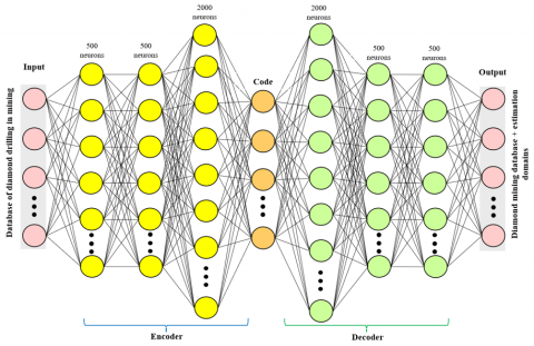
The specific architecture of the autoencoder neural network used in this research is detailed and visualized in Figure 1. The architecture of the autoencoder used in this study consists of an encoder and a decoder, each composed of multiple layers with ReLU activation functions. The encoder has four hidden layers with 600, 600, 800 and 10 neurons respectively. The decoder mirrors this structure and consists of four hidden layers with 800, 600, 600 and 10 neurons respectively. This symmetric architecture was chosen so that the autoencoder could learn a compressed representation of the input data in the middle layer and reconstruct the original data from this compressed representation. The autoencoder was trained using a mean square error loss function and the SGD optimizer with a learning rate of 0.2, over 100 epochs with a batch size of 128. After training the autoencoder, the K-Means algorithm with 30 initializations was applied to the encoded representations to form clusters. This architecture was chosen for its ability to effectively capture complex patterns in the data while ensuring computational efficiency.
Autoencoders transform categorical data into a continuous latent space, enabling the K-Means algorithm to operate more effectively. The encoder part of the autoencoder learns a compressed representation of the input data, including categorical variables, in a lower-dimensional space. This compressed representation is then used as input to the K-Means algorithm. While some information loss can occur due to the dimensionality reduction inherent in the encoding process, the architecture of the autoencoder is designed to retain the most salient features of the data, thereby minimizing the impact of any potential information loss.
Figure 1. Autoencoder neural networks
In the process of preparing to implement the autoencoder neural network, it is vital to develop a robust understanding of the underlying features of the available data. This is done through Exploratory Data Analysis (EDA), a crucial stage that allows elucidating key patterns, trends, and relationships within the dataset [35, 36]. In the study, the analysis focuses on the database of diamond drill holes, where critical variables include copper (Cu) and molybdenum (Mo) grades. The selected metrics for this analysis were the arithmetic mean, variance, standard deviation, kurtosis, and data correlation.
$\mu=\frac{1}{N} \sum_{i=1}^N x_i$ (4)
$\sigma^2=\frac{1}{N} \sum_{i=1}^N\left(x_i-\mu\right)^2$ (5)
$\sigma=\sqrt{\sigma^2}$ (6)
$Kurtosis =\frac{1}{N} \sum_{i=1}^N\left(\frac{x_i-\mu}{\sigma}\right)^4-3$ (7)
$Correlation (X, Y)=\frac{Covariance(X, Y)}{\sigma_x \sigma_y}$ (8)
Here, μ is the arithmetic mean, N is the total number of observations, $x_i$ is the value of the i-th observation, $\sigma^2$ is the variance, σ is the standard deviation, and $\sigma_x \sigma_y$ are the standard deviations of variables X and Y, respectively.
To determine the estimation domains in the present analysis, the K-Means clustering approach was employed. This method represents a prominent technique in the domain of unsupervised clustering, aiming to divide a dataset into K distinct and well-separated clusters. The process of identifying the optimal number of clusters is carried out by combining the elbow method and silhouette analysis [30]. The elbow method involves evaluating the sum of squares within the clusters (WCSS) for different values of K and selecting the value of K at the "elbow" of the graph. This is mathematically represented as:
$WCSS(K)=\sum_{i=1}^R \sum_{x \in C}\left\|x-\mu_i\right\|^2$ (9)
where, $\mu_i$ is the centroid of cluster $C_i$. In parallel, the silhouette method calculates the average silhouette score for different values of K, selecting the value that maximizes this score. The score is defined as:
$s(i)=\frac{b(i)-a(i)}{\max (a(i), b(i))}$ (10)
where, a(i) represents the average distance of point i to the other points in its cluster, and b(i) is the average distance of point i to the points in the nearest cluster outside of its own. Once the optimal number of clusters is selected, the K-Means algorithm is implemented through the following steps:
1. Initialization: Select K points as initial centroids.
2. Assignment: Assign each point to the cluster whose centroid is closest to it.
3. Update: Calculate new centroids as the average of the points in each cluster.
4. Convergence: Repeat the assignment and update steps until the centroids do not change significantly or a maximum number of iterations is reached [30].
The objective function is expressed as:
$J=\sum_{i=1}^k \sum_{x \in C_i}\left\|x-\mu_i\right\|^2$ (11)
where, $\mu_i$ is the centroid of cluster $C_i$ and k is the number of clusters.
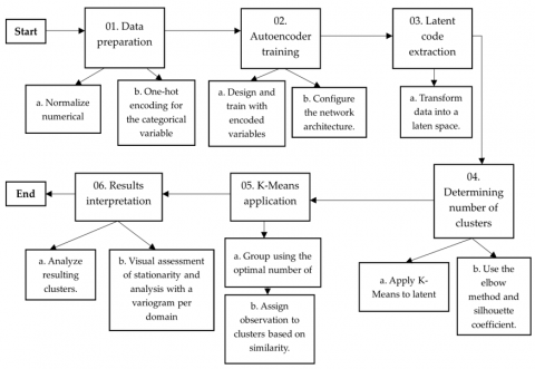
Figure 2 presents the sequence of stages that make up the design of this research.
Figure 2. Sequence of the research stages
3.1 Exploratory data analysis
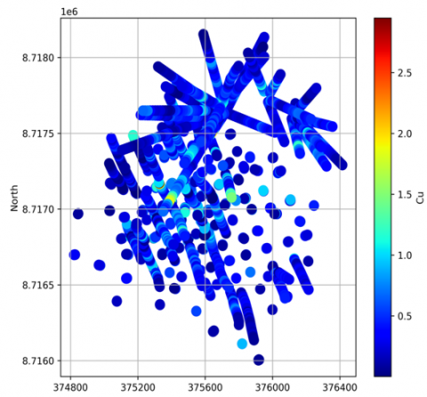
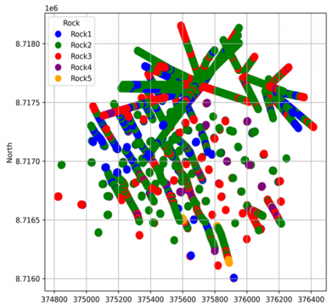
The aim of this research is to validate the use of the autoencoder neural network and K-Means clustering for the definition of geostatistical estimation domains through a practical application case. For this purpose, an exploratory data analysis was conducted on the database. Table 1 presents the statistics of the database, showing a total of 5,654 composites. The variables studied consist of east (x) coordinates, north (y) coordinates, elevation (z), as well as copper (Cu) and molybdenum (Mo) grades in per-centage (%), and finally, rock type. The codes assigned to the different rock types are Rock 1 for Magnetite Skarn, Rock 2 for Granodiorite, Rock 3 for Dacite Porphyry, Rock 4 for Calcareous Sediments, and Rock 5 for Catalina Volcanics. Figure 3 illustrates the distribution of the drill holes in the East-North directions, highlighting the copper and molybdenum grades and the specific rock type.
Table 1. Statistics of the diamond drill holes database
|
Description |
Easting (x) |
Northing (y) |
Elevation (z) |
Copper (Cu) |
Molybdenum (Mo) |
Rock Type |
|
Quantity |
5,654 |
5,654 |
5,654 |
5,654 |
5,654 |
5,654 |
|
Mean |
375,606.25 |
8,717,015.68 |
4,473.54 |
0.43 |
0.015 |
2.16 |
|
Std |
307.24 |
393.54 |
169.54 |
0.29 |
0.017 |
0.78 |
|
Minimum |
374,821.06 |
8,716,003.08 |
4,050.35 |
0.002 |
0.001 |
1 |
|
Q1 |
375,393.42 |
8,716,738.40 |
4,340.07 |
0.227 |
0.004 |
2 |
|
Q2 |
375,602.29 |
8,716,995.80 |
4,462.82 |
0.378 |
0.01 |
2 |
|
Q3 |
375,824.99 |
8,717,271.73 |
4,607.49 |
0.578 |
0.02 |
3 |
|
Maximum |
376,414.81 |
8,718,153.15 |
4,902.14 |
2.95 |
0.23 |
5 |
Table 2. Statistic of rock type with respect to the copper grade
|
Rock Type |
Quantity |
Mean |
Std |
Min (% Cu) |
Q1 |
Q2 |
Q3 |
Max |
Kur |
|
Magnetite Skarn |
906 |
0.36 |
0.28 |
0.002 |
0.18 |
0.31 |
0.48 |
1.87 |
3.13 |
|
Granodiorite |
3,317 |
0.48 |
0.31 |
0.003 |
0.27 |
0.43 |
0.65 |
2.95 |
3.26 |
|
Dacite Porphyry |
1,079 |
0.36 |
0.23 |
0.003 |
0.19 |
0.32 |
0.48 |
1.60 |
2.13 |
|
Calcareous Sediments |
307 |
0.35 |
0.21 |
0.051 |
0.21 |
0.31 |
0.47 |
1.89 |
8.35 |
|
Catalina Volcanics |
45 |
0.29 |
0.17 |
0.038 |
0.12 |
0.29 |
0.43 |
0.57 |
-1.38 |
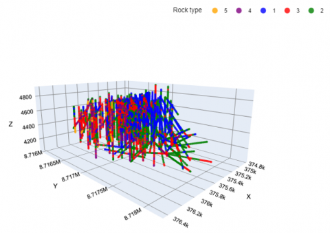
Table 2 summarizes statistical information on five different types of rocks, numbered from 1 to 5, including the number of observed samples, the mean, standard deviation (Std), Kurtosis (Kur), minimum values (Min), maximum values (Max), and the three quartiles (Q1, Q2, and Q3). It is noteworthy that rock 2 has the largest dataset (3,317), the highest mean and maximum values (0.48% and 2.95% copper, respectively). In contrast, rock 5, with only 45 data points, displays the lowest mean, maximum, and minimum values (0.29%, 0.57%, and 0.038% copper, respectively). The predominance of granodiorite rock in the studied area closely correlates with significant zones of copper mineralization, a characteristic feature of this type of igneous rock. This mineralogical association is further reinforced by the presence of other geological formations in the vicinity, such as magnetite skarns and dacite porphyries, collectively creating an environment conducive to copper concentration. Figure 4 displays an iso-metric view of the diamond drill holes in relation to the rock type.
(a) Diamond drill holes with respect to copper grade
(b) Diamond drill holes with respect to molybdenum grade
(c) Diamond drill holes with respect to rock type
Figure 3. East-North view of the diamond drill holes
Figure 4. Isometric view of diamond drill holes with respect to rock type
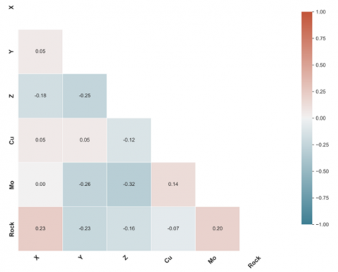
(a) Correlation matrix of database variables
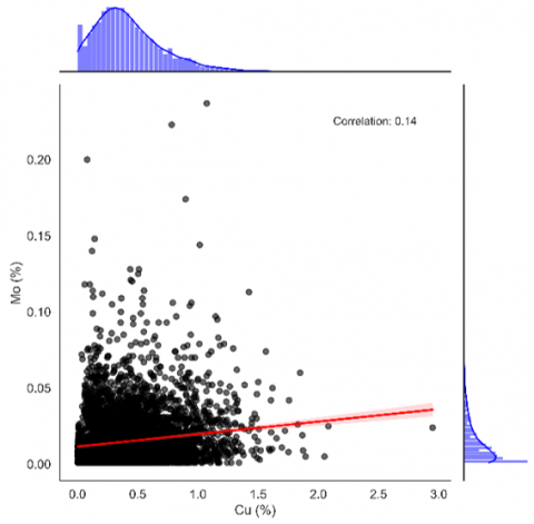
(b) Correlation of gold and molybdenum grades
Figure 5. Correlation of diamond drill hole database variables
Figure 5 displays a correlation matrix that encompasses all the variables contained in the initial database. It's crucial to highlight within this matrix the correlation between copper and molybdenum grades, which is estimated at 14%. Given this low coefficient, it is concluded that molybdenum does not influence the domain definition due to its dissimilar behavior relative to copper.
Figure 6. Copper grade distribution
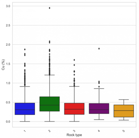
Figure 7. Boxplot of rock type with copper grades
Figure 6 displays the distribution of copper grades. In this graph, it is observed that these grades are predominantly concentrated in the range of 0.0 to 1.0%. Figure 7 presents a boxplot illustrating the distribution of copper grades in relation to different rock types. Specifically, for rock types 1 and 2, the concentration of copper grades stands out with values ranging between 1.0 and 3.0%.
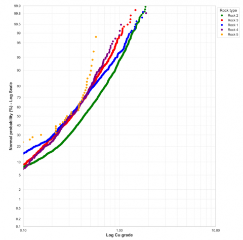
Figure 8 reveals the distribution of copper grades in relation to five different rock types. In this graph, there is a higher probability of high copper grades in rock type 2 and a lower probability of low grades in rock type 5.
Figure 8. Copper grade probability graph with rock type
3.2 Determination of the optimal number of clusters
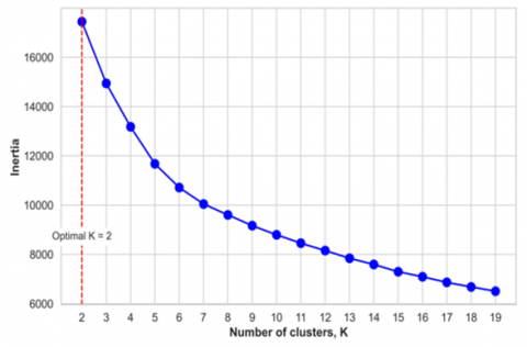
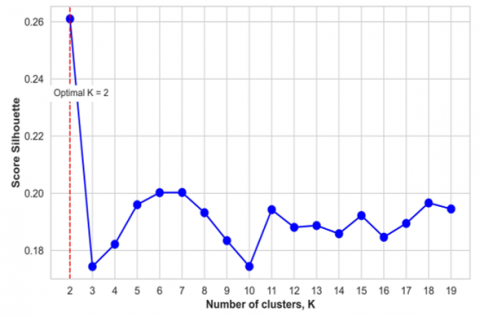
After normalizing the numeric variables: East coordinates (X), North coordinates (Y), elevation (Z), and copper grade (Cu), and encoding the categorical variable of rock type using the "one-hot" method, we proceeded with the training of Autoencoders. Subsequently, using the latent code, we determined the optimal number of clusters through two complementary techniques: the elbow method and the silhouette method. Figure 9 illustrates the results of the elbow method, identifying an optimal number of two clusters. This conclusion is based on the point where the graph shows a noticeable change in the curve, commonly known as the "elbow". Figure 10, on the other hand, represents the silhouette method, corroborating that the optimal number of clusters is also two, as indicated by the location of the peak in the data, i.e., the highest value in the silhouette graph. The agreement between these two methods strengthens the decision to segment the data into two estimation domains, providing a solid and methodologically robust foundation for subsequent analysis.
Figure 9. Elbow method
Figure 10. Silhouette method
In addition to the elbow method and silhouette method, we also considered the inertia and silhouette score for each number of clusters. Inertia, or the within-cluster sum of squares, measures the compactness of the clusters, with lower values indicating better clustering. The silhouette score measures how similar each data point is to its own cluster compared to other clusters, with higher values indicating better clustering. Both of these metrics were calculated for a range of cluster numbers, and the results were plotted to visually assess the optimal number of clusters. The optimal number of clusters was chosen as the one that minimized the inertia and maximized the silhouette score. Although the inertia for K=2 may seem relatively high compared to other cluster numbers, both the elbow method and silhouette score indicated that two is the optimal number of clusters. This suggests that two clusters provide a balance between cluster compactness, as measured by inertia, and separation, as measured by the silhouette score, thereby justifying our choice (see Table 3).
Table 3. Comparison of the results of the elbow method and silhouette method
|
Method |
Optimal Number of Clusters |
Inertia (K) |
Silhouette Score |
|
Elbow method |
2 |
17447.44 |
- |
|
Silhouette method |
2 |
- |
0.261 |
Table 4. Statistics of estimation domains and mineral grade
|
Domain |
Quantity |
Mean |
Std |
Min (% Cu) |
Q1 |
Q2 |
Q3 |
Max (% Cu) |
Kur |
|
1 |
4,204 |
0.44 |
0.30 |
0.002 |
0.22 |
0.39 |
0.60 |
2.95 |
5.21 |
|
2 |
1,450 |
0.41 |
0.25 |
0.01 |
0.24 |
0.36 |
0.52 |
2.09 |
5.07 |
3.3 Determination of estimation domains
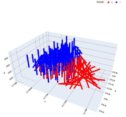
Table 4 presents a statistical analysis of the estimated domains in relation to the copper grade. Notably, domain one (1) houses the largest amount of data, totaling 4,204 data points. Within this domain, the copper grade varies, with a range extending from a minimum value of 0.002% to a maximum value of 2.95%. Meanwhile, domain two (2) consists of 1,450 data points and has an average copper grade of 0.41%. Figure 11 displays a visualization of the generated estimation domains.
Figure 11. Visualization of the estimation domains
Figure 12. Estimation domains silhouette score
Figure 12 presents the silhouette score of the estimation domains, which has a mean of 0.214. This value indicates moderate cohesion and separation between the identified clusters, suggesting an acceptable definition of the geologic domains. Table 5 shows additional metrics to support this claim, a mean Silhouette Score value of 0.21 and a Davies-Bouldin index of 1.70 indicating reasonably clear and distinct structuring between the clusters formed.
Table 5. Comparison of performance metrics of estimation domain definition models
|
Metric |
Value |
|
Medium Silhouette Score |
0.21 |
|
Davies-Bouldin Index |
1.70 |
Table 6 presents the comparisons of indicators of statistical significance tests, where the mean error for the Autoencoders Neural Networks (ANN) model is 0.29 with a variance error of 0.04 and a mean of the variances of the standardized errors of 0.04. In contrast, it was compared with the research of Boroh et al. [37], where they defined estimation domains with the classical method (geochemical modeling) which presented a mean error of 0.05, a variance error of 17.36 and a mean of the standardized error variances of 0.01. These results indicate that the ANN model has a superior performance in terms of mean error and error variance, suggesting that the observed improvements are not due to chance, but to the efficiency of the proposed model.
Table 6. Comparisons of indicators of statistical significance tests
|
Indicator |
Mean Error |
Variance Error |
Mean of the Variances of the Standardized Errors |
|
ANN |
0.29 |
0.04 |
0.04 |
|
Classical (Geochemical modeling) [37] |
0.05 |
17.36 |
0.01 |
Figure 13. Distribution of data in each geological domain of estimation with respect to rock type
Figure 14. Boxplot by estimation domain for copper grades
Figure 13 presents a box plot detailing the distribution of copper grades for each geological estimation domain. This chart not only illustrates how each domain controls the behavior of copper, but also provides essential information about the geological character underlying the definition of the domains. Figure 14 displays a probability plot that relates the estimation domains to the copper grade, offering a detailed view of trends within each domain. Domain 1 shows a higher probability of low copper grades, while domain 2 exhibits a higher probability of high copper grades.
Figure 15 presents a confusion matrix that quantifies the accuracy of the classification performed by the proposed methodology, which combines Artificial Neural Networks Autoencoders and K-Means. In domain 2, a high correspondence of 2,164.00 and 763.0 values is observed with the actual rock types 2 and 3, respectively. These numerical values represent the number of correct matches, indicating a higher accuracy in the correspondence between the estimated domains and the actual rock types. This validation provides an objective and robust evaluation of the efficiency of the clustering method, demonstrating its applicability and accuracy in defining geological estimation domains.
Figure 15. Confusion matrix showing accuracy of predicted domains and actual rock types using ANN Autoencoders and K Means
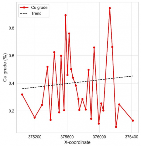
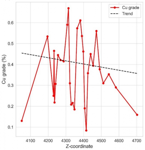
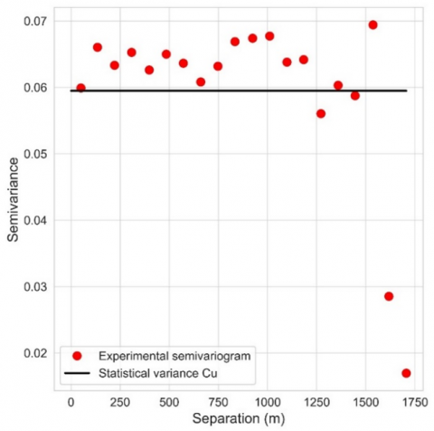
The domains D1 and D2 exhibit notable spatial continuity, a characteristic reflected in the omnidirectional semivariograms depicted in Figures 16 and 17. Domain 1 (D1) stands out for its initial continuity and a stationarity ranging from 0 to 500 meters, suggesting the presence of structures modeled with spherical or exponential shapes. Meanwhile, domain 2 (D2) demonstrates stationarity within the range of 0 to 600 meters, which is consistent with a spherical model due to its pronounced stationarity.
(a) Derived from the D1 domain at the X coordinate
(b) Derived from the D1 domain at the Y coordinate
(c) Derived from the D1 domain at the Z coordinate
(d) Onmidirectional semivariogram of the D1 domain
Figure 16. Drift and omnidirectional semivariogram of the domain D1
(a) Derived from the D2 domain at the X coordinate
(b) Derived from the D2 domain at the Y coordinate
(c) Derived from the D2 domain at the Z coordinate
(d) Onmidirectional semivariogram of the D2 domain
Figure 17. Drift and omnidirectional semivariogram of the domain D4
This research has clearly demonstrated the effectiveness of autoencoder neural networks and K-Means clustering in accurately defining geostatistical estimation domains. The silhouette score of 0.261 and an inertia of 17447.44 identified two optimal estimation domains, where domain 1 composed of 4204 samples with an average copper grade of 0.44% and domain 2 with a total of 1450 samples with an average grade of 0.41% copper. This analysis demonstrates a substantial improvement in terms of accuracy and efficiency, with a significantly lower average error (0.29 vs. 0.05) and a significantly reduced error variance (0.04 vs. 17.36) compared to geochemical modeling. Furthermore, the correlation of rock types with estimation domains underlines the geological relevance of this model, particularly in the association of 2534 granodiorite (rock 2) samples with domain 1 and the correspondence between rock types 2 and 3 in domains 1 and 2.
The application of this methodology contributes significantly to the field of geostatistics, fulfilling the essential requirements of local stationarity and modelable spatial structure for advanced methods such as Kriging. This integration not only maintains geological consistency, but also significantly optimizes the mineral resource estimation process. However, it is crucial to recognize the inherent limitations of the method, particularly the reliance on high-quality, error-free data, a common challenge in practical settings.
Looking to the future, there is a need to expand the database parameters to encompass additional aspects such as mineralization zones and metallurgical recovery rates. Such an expansion would not only improve the accuracy and applicability of the estimation domains, but also provide a more complete perspective of mineral potential. Additionally, exploration and comparison of alternative methodologies for domain definition, including advanced and traditional techniques, would reveal valuable insights into the strengths and weaknesses of each approach, opening avenues toward even greater optimization in mineral resource estimation and exploration.
|
h |
Encoded representation |
|
f |
Activation function |
|
W, V |
Weights |
|
b, c |
Bias |
|
x |
Input |
|
$\hat{\mathrm{x}}$ |
Reconstructed output |
|
g |
Activation function |
|
EDA |
Exploratory Data Analysis |
|
Cu |
Copper grade |
|
Mo |
Molybdenum grade |
|
N |
Number of observations |
|
xi |
Value of the i-th observations |
|
Q1, Q2, Q3 |
Quartiles statistics |
|
Kur |
Kurtosis |
|
a(i) |
Average distance of point i to other points in its cluster |
|
b(i) |
Average distance of point i to the points in the nearest cluster outside of its own |
|
Greek symbols |
|
|
µ |
Arithmetic mean |
|
$\sigma^2$ |
Variance |
|
$\sigma$ |
Standard deviation |
|
$\sigma_x \sigma_y$ |
Standard deviations of variables X and Y |
|
$\mu_i$ |
Centroid of cluster c-i |
[1] Resource, C.M. (2019). CIM Estimation of Mineral Resources & Mineral Reserves Best Practice Guidelines. Canadian Institute of Mining, Metallurgy and Petroleum: Westmount, QC, Canada.
[2] Rossi, M.E., Deutsch, C.V. (2013). Mineral resource estimation. Springer Science & Business Media. https://doi.org/10.1007/978-1-4020-5717-5
[3] Lara, R. (2020). Estimación de recursos minerales en dominios geometalúrgicos. Memoria para optar al título de Ingeniero Civil de Minas. Universidad de Concepción. Departamento de Ingeniería Metalúrgica (Inédito): Concepción. Retrieved from http://repositorio.udec.cl/xmlui/handle/11594/511.
[4] Emery, X., Ortiz, J.M. (2004). Defining geological units by grade domaining. Technical report, Universidad de Chile. Retrieved from https://www.researchgate.net/publication/254444133_Defining_Geological_Units_by_Grade_Domaining.
[5] Kapageridis, I., Apostolikas, A., Kamaris, G. (2021). Contact Profile analysis of resource estimation domains: A case study on a laterite nickel deposit. Materials Proceedings, 5(1): 89. https://doi.org/10.3390/materproc2021005089
[6] Matheron, G. (1963). Principles of geostatistics. Economic Geology, 58(8): 1246-1266. https://doi.org/10.2113/gsecongeo.58.8.1246
[7] Aisabokhae, J., Alimi, S., Adeoye, M., Oresajo, B. (2023). Geological structure and hydrothermal alteration mapping for mineral deposit prospectivity using airborne geomagnetic and multispectral data in Zuru Province, northwestern Nigeria. The Egyptian Journal of Remote Sensing and Space Science, 26(1): 231-244. https://doi.org/10.1016/j.ejrs.2023.02.005
[8] Abildin, Y., Xu, C., Dowd, P., Adeli, A. (2023). Geometallurgical Responses on lithological domains modelled by a hybrid domaining framework. Minerals, 13(7): 918. https://doi.org/10.3390/min13070918
[9] Abildin, Y., Xu, C., Dowd, P., Adeli, A. (2022). A hybrid framework for modelling domains using quantitative covariates. Applied Computing and Geosciences, 16: 100-107. https://doi.org/10.1016/j.acags.2022.100107
[10] Craigmile, P.F. (2014). A Review of traditional stationary Geostatistical Models. Statistics. Retrieved from https://bpb-us-w2.wpmucdn.com/u.osu.edu/dist/5/5306/files/2015/12/2014_SSES_stationary-2hlx8fe.pdf.
[11] Krumbein, W.C., Miller, R.L. (1953). Design of experiments for statistical analysis of geological data. The Journal of Geology, 61(6): 510-532. https://doi.org/10.1086/626125
[12] Moreira, C., Coimbra, J., Marques, D. (2020). Defining geologic domains using cluster analysis and indicator correlograms: A phosphate-titanium case study. Applied Earth Science, 129: 176-190. https://doi.org/10.1080/25726838.2020.1814483
[13] Adeli, A. (2018). Geostatistical modeling and validation of geological loggings and geological interpretations. Retrieved from https://repositorio.uchile.cl/handle/2250/168147.
[14] Adeli, A., Emery, X., Dowd, P. (2017). Geological modelling and validation of geological interpretations via simulation and classification of quantitative covariates. Minerals, 8(1): 7. https://doi.org/10.3390/min8010007
[15] Hernández, H., Alberdi, E., Goti, A., Oyarbide-Zubillaga, A. (2023). Application of the k-prototype clustering approach for the definition of geostatistical estimation domains. Mathematics, 11(3): 740. https://doi.org/10.3390/math11030740
[16] Mahjour, S.K., da Silva, L.O.M., Meira, L.A.A., Coelho, G.P., dos Santos, A.A.D.S., Schiozer, D.J. (2022). Evaluation of unsupervised machine learning frameworks to select representative geological realizations for uncertainty quantification. Journal of Petroleum Science and Engineering, 209: 109822. https://doi.org/10.1016/j.petrol.2021.109822
[17] de Castro Moreira, G., Modena, R.C.C., Costa, J.F.C.L., Marques, D.M. (2021). A workflow for defining geological domains using machine learning and geostatistics. Tecnologia em Metalurgia, Materiais e Mineração, 18. http://doi.org/10.4322/2176-1523.20212472
[18] Li, Y., Chu, X., Tian, D., Feng, J., Mu, W. (2021). Customer segmentation using K-Means clustering and the adaptive particle swarm optimization algorithm. Applied Soft Computing, 113: 107924. https://doi.org/10.1016/j.asoc.2021.107924
[19] Peralta, M., Merma, J., Chavez, E., Soto, C., Jimenez, W. (2022). Aplicación del Algoritmo K-Means en estudiantes universitarios del área de sistemas e informática para caracterizar la salud mental, durante el aislamiento en COVID-19. Memorias de la Vigésima Primera Conferencia Iberoamericana en Sistemas, Cibernética e Informática (CISCI). https://doi.org/10.54808/CISCI2022.01.92
[20] Barba, R., Guerrero, H., Salazar, J. (2016). Análisis de clústeres para la clasificación de datos económicos. Revista Publicando, 3(7): 267-275. https://revistapublicando.org/revista/index.php/crv/article/view/249.
[21] de Castro Moreira, G., Costa, J.F.C.L., Marques, D.M. (2021). Applying Clustering Techniques and Geostatistics to the Definition of Domains for Modelling. In International Geostatistics Congress, Cham: Springer International Publishing, pp. 199-219. https://doi.org/10.1007/978-3-031-19845-8_16
[22] Eshimiakhe, D., Lawal, K. (2022). Application of K-means algorithm to Werner deconvolution solutions for depth and image estimations. Heliyon, 8(11): e11665. https://doi.org/10.1016/j.heliyon.2022.e11665
[23] Zhao, Y., Zhou, X. (2021). K-Means clustering algorithm and its improvement research. In Journal of Physics: Conference Series, 1873(1): 012074. https://doi.org/10.1088/1742-6596/1873/1/012074
[24] Li, Y., Wu, H. (2012). A clustering method based on K-means algorithm. Physics Procedia, 25: 1104-1109. https://doi.org/10.1016/j.phpro.2012.03.206.
[25] Morissette, L., Chartier, S. (2013). The K-Means clustering technique: General considerations and implementation in Mathematica. Tutorials in Quantitative Methods for Psychology, 9(1): 15-24. https://doi.org/10.20982/tqmp.09.1.p015
[26] Chen, S., Guo, W. (2023). Auto-encoders in deep learning-A review with new perspectives. Mathematics, 11(8): 1777. https://doi.org/10.3390/math11081777
[27] Michelucci, U. (2022). An introduction to autoencoders. arXiv preprint arXiv:2201.03898. https://doi.org/10.48550/arXiv.2201.03898
[28] Sokolovsky, M.J. (2018). Designing convolutional neural networks and autoencoder architectures for sleep signal analysis (Doctoral dissertation, PhD Thesis. Worcester: Worcester Polytechnic Institute). Retrieved from https://web.wpi.edu/Pubs/ETD/Available/etd-042318-010544/unrestricted/msokolovsky.pdf.
[29] Baldi, P. (2012). Autoencoders, unsupervised learning, and deep architectures. In Proceedings of ICML Workshop on Unsupervised and Transfer Learning, JMLR Workshop and Conference Proceedings, pp. 37-49. https://proceedings.mlr.press/v27/baldi12a.html.
[30] Saputra, D.M., Saputra, D., Oswari, L.D. (2020). Effect of distance metrics in determining k-value in K-Means clustering using elbow and silhouette method. In Sriwijaya International Conference on Information Technology and Its Applications (SICONIAN 2019), Atlantis Press, pp. 341-346. http://doi.org/10.2991/aisr.k.200424.051
[31] Umargono, E., Suseno, J.E., Gunawan, S.V. (2020). K-Means clustering optimization using the elbow method and early centroid determination based on mean and median formula. In the 2nd International Seminar on Science and Technology (ISSTEC 2019), Atlantis Press, pp. 121-129. https://doi.org/10.2991/assehr.k.201010.019
[32] Delong, Ł., Kozak, A. (2023). The use of autoencoders for training neural networks with mixed categorical and numerical features. ASTIN Bulletin: The Journal of the IAA, 53(2): 213-232. https://doi.org/10.1017/asb.2023.15
[33] Mahapatra, D., Amrit, P., Singh, O.P., Singh, A.K., Agrawal, A.K. (2023). Autoencoder-convolutional neural network-based embedding and extraction model for image watermarking. Journal of Electronic Imaging, 32(2): 021604-021604. https://doi.org/10.1117/1.JEI.32.2.021604.
[34] Kiwelekar, A.W., Mahamunkar, G.S., Netak, L.D., Nikam, V.B. (2020). Deep learning techniques for geospatial data analysis. Machine Learning Paradigms: Advances in Deep Learning-Based Technological Applications, 63-81. https://doi.org/10.1007/978-3-030-49724-8_3
[35] Abzalov, M. (2016). Exploratory data analysis. In Applied Mining Geology, 12. https://doi.org/10.1007/978-3-319-39264-6_15
[36] De Fouquet, C. (2011). From exploratory data analysis to geostatistical estimation: Examples from the analysis of soil pollutants. European Journal of Soil Science, 62(3): 454-466. https://doi.org/10.1111/j.1365-2389.2011.01374.x
[37] Boroh, A.W., Sore, G.K., Ayiwouo, N.M., Gbambie, M. I., Ngounouno, I. (2021). Implication of geological domains data for modeling and estimating resources from Nkout iron deposit (South-Cameroun). Journal of Mining and Metallurgy A: Mining, 57(1): 1-17. https://doi.org/10.21203/rs.3.rs-270923/v1