Jose Rizal*![]() | Agus Y. Gunawan
| Agus Y. Gunawan![]() | Siska Yosmar
| Siska Yosmar![]() | Aang Nuryaman
| Aang Nuryaman![]()
© 2024 The authors. This article is published by IIETA and is licensed under the CC BY 4.0 license (http://creativecommons.org/licenses/by/4.0/).
OPEN ACCESS
The research area of the present study is the Sumatra megathrust zone, which can be partitioned into five segments based on the large earthquake sources, including the Aceh Andaman, Nias Simeulue, Mentawai Siberut, Mentawai Pagai, and Enggano segments. This work presents the recognition of seismicity patterns in the research area from January 1970 to December 2022 using segmental and zonal mathematical modeling of the annual maximum earthquake magnitude. To achieve this, we use two kinds of Gaussian mixture models: G-group Gaussian independent mixture models (G-group GMMs) and N-state Gaussian hidden Markov models (N-state GHMMs) to determine the appropriate probability density function of the seismicity data (ePDF). The fit model is selected based on the smallest Bayes information criterion. For the segment analysis, the results show that the ePDF of the Mentawai-Pagai segment fits the 2-state GHMM, whereas, for the four remaining segments, it tends to fit the 2-group GMM. Subsequently, for the zone analysis, the ePDF of the data fits the 2-state GHMM. Thus, from a segmental and zoning point of view, seismicity patterns fluctuate at two levels. From a seismic risk management aspect, these findings can be used to evaluate the risk vulnerability of an area to destructive earthquakes. That is, the patterns of seismicity sequences in all segments of the Sumatra megathrust zone all fluctuate within the range of moderate to strong earthquakes. Furthermore, the seismicity pattern in the Mentawai-Pagai segment and the Sumatra megathrust zone has Markov properties.
maximum earthquake magnitude, seismicity patterns, gaussian distribution, mixture models, Markov properties
The seismicity pattern is a variation of sensitive stress indicators of underground dynamics due to earthquake events. The estimation model of seismicity pattern, especially for a subduction zone, can be analyzed based on geodetic strain level, geomechanical parameters, and the earthquake catalog [1]. Whereas the methods used are very varied, to name a few: the Region-Time-Length (RTL) method [2], the Epidemic-Type Aftershock-Sequences (ETAS) model [3], the Pattern Informatics (PI) method [4], the Z-value method [5], and probabilistic methods [6-14].
The probabilistic methods to identify the Sumatra seismicity patterns have been previously provided by Orfanogiannaki et al. [6] and Rizal et al. [12] using the Poisson Hidden Markov Models (PHMMs) that correspond to the earthquake catalog, i.e., earthquake frequency. Their study was motivated by two major earthquake events, 26 December 2004 and 28 March 2005, with moment magnitudes of Mw 9.1 and Mw 8.6, respectively. Orfanogiannaki et al. [6] presented seismic patterns both segmentally and zonally (in 23-day periods) in their article, where the optimum number of seismic levels for each subregion was found to be different from two to four categories. The same study of seismic patterns in the Sumatra megathrust zone after the occurrence of two earthquakes on December 26, 2004 and March 28, 2005, has also been carried out by Mignan et al. [15], Dasgupta et al. [16], and Dewey et al. [17].
In our previous study, Rizal et al. [12], we implemented the same procedure as in Orfanogiannaki et al. [6] to observe seismicity patterns in the Sumatra megathrust subduction zone by taking different earthquake data and observation periods. Notice that, in Rizal et al. [12], the characteristics of earthquake data were magnitude thresholds Mw=5 with time of observation 1973-2018, and results showed that the optimum number of levels of local seismic patterns varied from two to six categories due to strong overdispersion relative to Poisson distribution. However, Orfanogiannaki et al. [6] and Rizal et al. [12] assumed that the data were spatially independent. Here, an interesting research question to examine is whether the frequency data from those two selected segments considered by Orfanogiannaki et al. [6] and Rizal et al. [12] may have spatial dependencies. If that happens, the analysis may not be carried out segmentally. Therefore, to overcome this issue, we need to provide alternative seismic data along with its modeling that can be used to identify seismic patterns and does not contain spatial dependencies.
As we know, the method of Kendall’s rank correlation is used to analyze the spatial dependency of two variables. This method is more appropriate for bivariate discrete variable due to adjustments for ties condition, as stated by Denuit and Lambert [18], and will be applied to the pairs of segmentation data modeled (see Table 1). There are three types of Kendall’s rank correlation, namely τa, τb, and τc. A brief explanation of the three types is as follows. Kendall’s rank correlation τa and τb are typically applied to square tables and τb will adjust for tied ranks. Additionally, rectangular tables are frequently utilized with τc. A detailed explanation of the three types of Kendall’s rank correlation can be seen by Somers [19].
The hypothesis for testing the dependence of two data pairs of discrete variables is as follows: H0: τb=0 (independent) vs H1: τb≠0 (dependent), where we reject H0 if the p-value <0.05. As we can see in Table 1, the ten tested data pairs have a p-value <0.05. Accordingly, it can be concluded that H0 is rejected or that there is a spatial dependency between each pair of data. This condition has the consequence that we cannot analyze seismicity patterns segmentally.
The frequency of earthquake data is commonly used by many researchers as an object for dealing with seismicity patterns. We note, however, that the frequency data may give no information concerning earthquake coordinates or their magnitude, which may become important for further earthquake prediction. In this study, we propose an alternative earthquake catalog, that is, the maximum observed earthquake magnitude, as an object to analyze seismicity patterns since it maintains earthquake information such as its coordinates and magnitude. Another benefit is that the characteristics of the data are not too heterogeneous due to the fact that the maximum observed earthquake magnitude data range is narrower than earthquake frequency data. The maximum observed earthquake magnitude data has already been suggested by Tsapanos and Christova [20] and Tsapanos [21] to evaluate the seismicity patterns and seismic hazards.
In this paper, we use the maximum observed earthquake magnitude to identify seismic patterns in the Sumatra megathrust zone and at the sources of large earthquakes in that zone. This study has not been included in the Indonesian national seismic hazard map compiled by Irsyam et al. [22].
Table 1. Dependence measure for two pairs of earthquake frequency data in the Sumatra megathrust zone
|
Segments |
Nias Simeulue (NS) |
Mentawai Siberut (MS) |
Mentawai Pagai (MP) |
Enggano (EO) |
||||
|
$\hat{\boldsymbol{\tau}}_{\boldsymbol{b}}$ |
p-value |
$\hat{\boldsymbol{\tau}}_{\boldsymbol{b}}$ |
p-value |
$\hat{\boldsymbol{\tau}}_{\boldsymbol{b}}$ |
p-value |
$\hat{\boldsymbol{\tau}}_{\boldsymbol{b}}$ |
p-value |
|
|
Aceh Andaman (AA) |
0.683 |
0.000 |
0.565 |
0.000 |
0.391 |
0.000 |
0.339 |
0.001 |
|
Nias Simeulue (NS) |
|
|
0.524 |
0.000 |
0.570 |
0.000 |
0.413 |
0.000 |
|
Mentawai Siberut (MS) |
|
|
|
|
0.285 |
0.008 |
0.249 |
0.019 |
|
Mentawai Pagai (MP) |
|
|
|
|
|
|
0.323 |
0.002 |
Since the maximum earthquake magnitude data gives continuous data, the Gaussian distribution can be applied to identify the seismicity patterns. However, we have to realize that in some cases, the Gaussian distribution cannot properly capture the dynamics of the probability of empirical data due to heterogeneity in the main data, in which the heterogeneity can be related to the dynamic of seismic activity, as stated by Orfanogiannaki et al. [6], Votsi et al. [7], Orfanogiannaki et al. [8], Yip et al. [11], and Rizal et al. [12-14]. To deal with heterogeneity, the G-group Gaussian independent mixture models (G-group GMMs) [23] and N-state Gaussian Hidden Markov mixture models (N-state GHMMs) [24, 25] can be applied, where the parameters of the models are estimated using the Expectation-Maximization (EM) algorithm provided by Dempster et al. [26].
Subsequently, we note that some other mathematical models can be used in pattern recognition issues, namely K-Nearest Neighbor (K-NN) [27], Pearson mixture modeling [28], and linear mixture models [29]. However, we do not use these three models due to the weaknesses in each model. A few disadvantages and difficulties associated with K-NN include high processing costs, sluggish performance, memory and storage problems for large datasets, sensitivity to the choice of “K”, and vulnerability to the curse of dimensionality. Meanwhile, some disadvantages for Pearson and linear mixture models are issues that come with utilizing the standard correlation structure, interpretation of the model parameters, and computational problems [30].
The purpose of this study is to recognize and analyze seismicity patterns in the Sumatra megathrust zone, which includes the Aceh-Andaman, Nias-Simeulue, Mentawai-Siberut, Mentawai-Pagai, and Enggano segments, using mathematical modeling of the annual maximum earthquake magnitude. To do so, we employ two mixture models: G-group GMMs and N-state GHMMs, to determine the appropriate probability density function of the study data.
The paper is organized as follows: In Section 2, we explain the data and the mixture models used in this work. A general description of G-group GMMs and N-state GHMMs, including the EM algorithm for estimating the parameters of the models, is presented in Subsections 2.1 and 2.2. Furthermore, to assist seismologists in comprehending our study, we discuss the research methodology in Section 3. Meanwhile, in Section 4, we report the results of the data analysis and some discussions concerning the relevancy of the present results to other studies. In the last section, conclusions and future research are written.
Let the random variable $\mathcal{M}_{\max }^{\text {obs }}$ be the maximum observed earthquake magnitude (in $\mathrm{M}_{\mathrm{w}}$) occurring in sequential time intervals of duration one year. The historical realization data of $\left\{\mathcal{M}_{\max _t}^{\text {obs }}: t \in[1970,1974, \cdots, 2022]\right\}$ was obtained from earthquake catalog data published online by the United States Geological Survey (USGS). There are several variations of the type magnitude in the earthquake catalog that we use, namely: body magnitude $\left(\mathrm{m}_{\mathrm{b}}\right)$, surface-wave magnitude $\left(\mathrm{M}_{\mathrm{s}}\right)$, and magnitude momen $\left(\mathrm{M}_{\mathrm{w}}\right)$. Therefore, before analyzing the data, it is necessary to convert the earthquake magnitude into $\mathrm{M}_{\mathrm{w}}$ type. Here, the type conversion magnitude refers to Irsyam et al. [22], where the conversion method used is analogous to the method applied by Kadirioğlu and Kartal [31].
Figure 1. (a) A map of the Andaman and the Sumatra megathrust zones (marked by an orange box), meanwhile; (b) A map of the five large earthquake sources in these zones, with the potential of a magnitude-maximum earthquake (Mmax)
Our research area is the Sumatra megathrust zone (see Figure 1(a)). This region is part of the Sunda megathrust subduction zone, which includes the Andaman megathrust, Sumatra megathrust, and Java megathrust [32]. According to Irsyam et al. [22], there are five subduction segments in the research area. Therefore, to obtain the pattern of seismicity, we analyze data in two scenarios: segmentally and zonally. Additionally, Figure 1(b) represents the identity and potential of the maximum earthquake magnitude of the five subduction segments. For the next discussion, we elaborate G-group GMMs and $\mathrm{N}$-state GHMMs, including the implementation of the EM algorithm to estimate the parameters of the model in subsections 2.1 and 2.2 , respectively. In this paper, the resulting number of groups in GMMs and the number of states in GHMMs will be associated with the number of seismicity patterns that are classified into six categories, referring to Duda and Nuttli [33], namely minor ($3 \leq M_w<3.9$), light ($4 \leq M_w$ $<4.9$), moderate ($5 \leq M_w<5.9$), strong ($6 \leq M_w<6.9$), major (7 $\left.\leq \mathrm{M}_{\mathrm{w}}<7.9\right)$, and great $\left(\mathrm{M}_{\mathrm{w}} \geq 8.0\right)$.
2.1 Gaussian independent mixture models (GMMs)
Let us assume that the random variable $M_{\text {max }}^{\text {obs }}$ follows the distribution of GMMs with the number of groups $G$, which is abbreviated as $G$-group GMMs. The probability density function (PDF) $M_{\max }^{\text {obs }}$ can be formulated as follows:
$\operatorname{Pr}\left(M_{\max }^{\mathrm{obs}}=m_t\right)=\sum_{g=1}^{\mathrm{G}} \delta_g \mathrm{~N}_g\left(m_t ;\left(\mu_g, \sigma_g\right)\right)$ (1)
The parameter $\delta_g$ is the weight of the $g$ component satisfying $0 \leq \delta_g \leq 1$ and $\sum_{g=1}^{\mathrm{G}} \delta_g=1$. The notation $N_g\left(m_t ;\left(\mu_g, \sigma_g\right)\right)$ is a probability density of the Gaussian distribution, with the parameters expressing the average $\mu_g$ and variance $\sigma_g$ of the $g$ component.
The parameters estimation ($\boldsymbol{\theta}=\left\{\delta_g, \mu_g, \sigma_g, g=1,2, \ldots, \mathrm{G}\right\}$) are obtained by solving the problem of maximizing the loglikelihood function for complete data of Eq. (1), which can be written as follows:
$\begin{gathered}\mathcal{L}_{E M}(\boldsymbol{\theta})=\sum_{t=1}^{\mathrm{T}} \log \operatorname{Pr}\left(\left(m_t, z_t\right) ; \boldsymbol{\theta}\right) =\sum_{t=1}^{\mathrm{T}} \log \left(\sum_{g=1}^{\mathrm{G}} \delta_g \mathrm{~N}_g\left(\left(m_t, z_t\right) ;\left(\mu_g, \sigma_g\right)\right)\right)\end{gathered}$ (2)
the unobserved variable $Z_t$ in Eq. (2) is define as follows:
$z_t(g)= \begin{cases}1 & \text { if } m_t \text { is in the group } g \\ 0 & \text { others. }\end{cases}$ (3)
where, $Z_t(g)$ is assumed to be mutually independent and has an identical distribution which places the $t$ observation data belongs to the group $g$.
The EM index on $\mathcal{L}_{E M}(\boldsymbol{\theta})$ in Eq. (2) means that the method used to obtain the estimated parameter $\boldsymbol{\theta}$ is the EM algorithm due to the presence of unobserved variables in the main data [26]. The estimation of the parameter $\boldsymbol{\theta}$ of GMMs is obtained by calculating the expectation of Eq. (2) as follows:
$\begin{gathered}\mathcal{H}_{E M}\left(\boldsymbol{\theta}, \boldsymbol{\theta}^{l-1}\right)= \\ \mathrm{E}\left[\mathcal{L}_{E M}\left(\boldsymbol{\theta} \mid m_t, \boldsymbol{\theta}^{l-1}\right)\right]=\sum_{t=1}^{\mathrm{T}} \sum_{g=1}^{\mathrm{G}} r_{t g} \log \delta_g+ \sum_{t=1}^{\mathrm{T}} \sum_{g=1}^{\mathrm{G}} r_{t g} \log \mathrm{N}\left(m_t ;\left(\mu_g, \sigma_g\right)\right),\end{gathered}$ (4)
where, $l$ expresses the iteration and $r_{t g}=\operatorname{Pr}\left(z_t=g \mid m_t\right)$ is the maximum posterior probability value of $m_t$ on group $g$. At the E-step of the EM algorithm, it is sufficient to calculate the $r_{t g}$, while for M-step we maximize the objective function of $\mathcal{H}_{E M}\left(\boldsymbol{\theta}, \boldsymbol{\theta}^{l-1}\right)$ on the parameter $\delta_g, \mu_g, \sigma_g$.
In the next subsection, we proceed with an explanation of the GHMMs and estimation model parameters using the EM algorithm. Since the unobserved variable from the random variable $M_{\max }^{\text {obs }}$ has Markov properties, the structures of GHMMs are more complex than GMMs. Thus, a more detailed explanation to this model is required.
2.2 Gaussian hidden Markov models (GHMMs)
The Hidden Markov Models (HMMs) used in this study consist of two parts. Adapted to the problem of this research, the first part $\left\{C_t: t \in \mathrm{T}\right\}$ is a parameter process where the state space is unobserved, namely the seismicity patterns, and has Markov properties. The second part $\left\{M_{\max _t}^{\mathrm{obs}}: t \in \mathrm{T}\right\}$ is a continuous process that is observed, and the $M_{\max _t}^{\mathrm{obbs}}$ distribution depends only on $C_t$. More formally, HMMs can be formulated as in Eqs. (5) and (6) [34].
$\begin{aligned} & \operatorname{Pr}\left(C_t=c_t \mid \boldsymbol{C}^{(t-1)}=\boldsymbol{c}^{(t-1)}\right) \quad=\operatorname{Pr}\left(C_t=c_t \mid C_{t-1}=c_{t-1}\right)\end{aligned}$ (5)
$\begin{aligned} & \operatorname{Pr}\left(M_{\max _t}^{\mathrm{obs}}=m_t {\mid M_{\max }^{\mathrm{obs}}}^{(t-1)}=\boldsymbol{m}^{(t-1)}, \boldsymbol{C}^{(t)}=\boldsymbol{c}^{(t)}\right) =\operatorname{Pr}\left(M_{\max _t}^{\mathrm{obs}}=m_t \mid C_t=c_t\right) \\ & \end{aligned}$ (6)
In the present paper, $\boldsymbol{m}^{(\mathrm{t})}=\left(m_1, m_2, \ldots, m_{\mathrm{t}}\right)$ and $\boldsymbol{c}^{(\mathrm{t})}=\left(c_1, c_2, \ldots\right.$, $c_{\mathrm{t}}$) express the vector realization value of random variables $\boldsymbol{M}_{\max }^{\text {obs }}(t)=\left(M_{\max _1}^{\mathrm{obs}}, M_{\max _2}^{\mathrm{obs}}, \cdots, M_{\max _t}^{\mathrm{obs}}\right)$ and $\boldsymbol{C}^{(\mathrm{t})}=\left(C_1, C_2, \cdots, C_{\mathrm{t}}\right)$, respectively. Accordingly, if the Markov chain $\left\{C_t\right\}$ has a finite number of values $\{1,2, \ldots, N\}$ and each observation of $M_{\text {max }}^{\text {obs }}$ is generated by one of $N$ Gaussian distribution, then we call $\left\{M_{\max _t}^{\text {obs }}\right\}$ an N-state GHMMs.
Previously, we define $p_i$ as the probability density function of $M_{\max t}^{\mathrm{obs}}$ if the Markov chain at time $t$ is in state $i$, which is $p_i(m)=\operatorname{Pr}\left(M_{\max _t}^{\mathrm{obs}}=m \mid C_t=i\right)$. Subsequently, we also define $\mathbf{P}(m)$ as the diagonal matrix with $i$ th diagonal element $p_i(m)$. Suppose that $\left\{m_1, m_2, \ldots, m_T\right\}$ follow the $\mathrm{N}$-state GHMMs with initial distribution $\boldsymbol{\delta}, \boldsymbol{P}(m)$, and $\boldsymbol{\Gamma}$ transition probability matrix from the state space $\left\{C_t\right\}$, the likelihood function of the GHMMs with $N$ state is formulated as follows:
$\begin{gathered}\mathcal{Q}_{\mathrm{T}}=\left(\boldsymbol{M}_{\max }^{\mathrm{obs}}(\mathrm{T})=\boldsymbol{m}^{(\mathrm{T})}\right) =\boldsymbol{\delta} \mathbf{P}\left(m_1\right) \boldsymbol{\Gamma} \mathbf{P}\left(m_2\right) \boldsymbol{\Gamma} \mathbf{P}\left(m_3\right) \cdots \boldsymbol{\Gamma P}\left(m_{\mathrm{T}}\right) \mathbf{1}^{\prime}\end{gathered}$ (7)
By using the concept of directed graphical model referring to Jordan [35] and consider Eq. (7), the logarithm of the joint distribution from set $\left(\boldsymbol{M}_{\max }^{\text {obs }}{ }^{(\mathrm{T})}, \boldsymbol{C}^{(\mathrm{T})}\right)$ is given by:
$\begin{gathered}\log \left(\operatorname{Pr}\left(\boldsymbol{M}_{\max }^{\text {obs }}(\mathrm{T}), \boldsymbol{c}^{(\mathrm{T})}\right)\right)= \\ \log \left(\delta_{c_1} \prod_{t=2}^{\mathrm{T}} \gamma_{c_{t-1}, c_t} \prod_{t=1}^{\mathrm{T}} \operatorname{Pr}_{c_t}\left(m_t\right)\right)=\log \delta_{c_1}+ \sum_{t=2}^{\mathrm{T}} \log \gamma_{c_{t-1}, c_t}+\sum_{t=1}^{\mathrm{T}} \log \operatorname{Pr}_{c_t}\left(m_t\right) .\end{gathered}$ (8)
In the $\mathrm{N}$-state $\mathrm{GHMMs}$, the $\mathrm{EM}$ algorithm treats the transition probability matrix and a collection of states as missing data. Because of this, we must first define two random variables, $u_j(t)$ and $v_{j k}(t)$, using the zero-one random variables that represent the states $c_1, c_2, \ldots, c_n$. When the model's state is $j$ at time $t$, the random variable $u_j(t)$ equals 1; otherwise, $t=1$, $2, \ldots, T$. On the other hand, the random variable $v_{j k}(t)$ equals 0 for $t=2,3, \ldots, T$, and 1 if $c_{t-1}=j$ and $c_t=k$. Next, we obtain the complete log-likelihood data of the GHMMs from Eq. (8) using two random variables, $u_j(t)$ and $v_{j k}(t)$ :
$\begin{aligned} \log \left(\operatorname{Pr}\left(\boldsymbol{M}_{\max }^{\mathrm{obs}}, \boldsymbol{C}^{(\mathrm{T})}\right)\right)=\sum_{j=1}^N u_j(1) \log \delta_j+ \sum_{j=1}^N \sum_{k=1}^N\left(\sum_{t=2}^{\mathrm{T}} v_{j k}(t)\right) \log \gamma_{j k}+ \sum_{j=1}^N \sum_{t=1}^{\mathrm{T}} u_j(t) \log \operatorname{Pr}_j\left(m_t\right) . \\ & \end{aligned}$ (9)
At the E-step of the EM algorithm, we calculate the conditional expectation of the missing data given an observation and determine the estimated initial value for the GHMMs model parameters. Technically, replace all the quantities $u_j(t)$ and $v_{j k}(t)$ by their conditional expectations given the observations $\boldsymbol{M}_{\max }^{\mathrm{obss}}$:
$\hat{u}_j(t)=\operatorname{Pr}\left(C_t=j \mid \boldsymbol{m}^{(\mathrm{T})}\right)=\alpha_t(j) \beta_t(j) / \mathcal{Q}_{\mathrm{T}}$ (10)
$\begin{gathered}\hat{v}_{j k}(t)=\operatorname{Pr}\left(C_{t-1}=j, C_t=\right. \\ \left.k \mid \boldsymbol{m}^{(\mathrm{T})}\right)=\alpha_{t-1}(j) \gamma_{j k} p_k\left(m_t\right) \beta_t(k) / \mathcal{Q}_{\mathrm{T}}\end{gathered}$ (11)
where, $\quad \alpha_t(j)=\operatorname{Pr}\left(\boldsymbol{M}_{\max }^{\mathrm{obs}}(\mathrm{t}), C_t=j\right) \quad$ and $\quad \beta_t(i)=$$\operatorname{Pr}\left(\boldsymbol{M}_{\max _{t+1}}^{\mathrm{obs}^{(\mathrm{T})}}=\boldsymbol{m}_{t+1}^{(\mathrm{T})} \mid C_t=i\right)$. At the M-step of the EM algoritm we maximize the complete data log-likelihood function Eq. (9), with respect to the three sets of parameters: $\delta, \Gamma$, and the parameter of the state-dependent distributions [34].
To help the earthquake researchers better understand our work, the methodology of the research is presented here. In this section, we explain the procedure to get the maximum observed earthquake magnitude (research data), the Gaussian mixture models used, and the criteria for model selection.
The steps listed below can be followed to get the research data modeled:
(1) Obtaining the initial seismicity data from one earthquake catalog website, namely https://earthquake.usgs.gov.
(2) Converting the various type magnitudes in the earthquake catalog that we get in point one into Mw type.
(3) Preparing seismicity data for mathematical modeling through the declustering process (i.e., separating the mainshock with foreshock and aftershock earthquakes), and estimating the magnitude of completeness (Mc).
(4) Collecting the data from point three to obtain the annual maximum earthquake magnitude.
Subsequently, we apply the GMMs and the GHMMs to obtain seismicity patterns for all segments in the Sumatra megathrust zone. To achieve this, we use a trial-and-error process for several values of the number of groups or states that are feasible to be tested.
The optimum number of groups or states is selected based on the smallest Bayes Information Criterion (BIC). The formulation of BIC is defined as follows:
$\mathrm{BIC}=\log \operatorname{Pr}\left(\boldsymbol{m}^{(\mathrm{T})} \mid \widehat{\boldsymbol{\theta}}\right)-\frac{1}{2} n(\widehat{\boldsymbol{\theta}}) \log (\mathrm{T})$ (12)
The variable $n(\widehat{\boldsymbol{\theta}})$ is the number of parameters estimated and $\log \operatorname{Pr}\left(\boldsymbol{m}^{(\mathrm{T})} \mid \widehat{\boldsymbol{\theta}}\right)$ is the maximized log-likelihood function for complete data [36].
As an illustration of our research, we use the seismicity data from January 1970 to December 2022 of the Sumatra megathrust zone, published online by the United States Geological Survey (USGS). The information related to the identity, custom rectangle, instrumental earthquake catalogs (i.e., the magnitude of completeness (Mc), the productivity of the earthquakes (a), and the proportionate distribution of large and small earthquakes (b)) and statistical description (max, mean, and variance) of the research data are shown in Table 2.
Table 2. Some information related to the identity, coordinates of the research area, and statistical information from historical data of the maximum earthquake magnitude from 1970-2022
| Identity of Research Area | Custom Rectangle of Research Area | Estimating the Mc (Mw), a, and b for the Earthquake Catalogs Studied | Empirical Earthquake Magnitude (Mw) | ||||||
| Latitude | Longitude | Mc | a | b | Max | Mean | Variance | ||
| Segments | Aceh Andaman (AA) | [2.2, 7.0] | [92, 97] | 4.5 | 8.18 | 1.07 ± 0.02 | 9.1 | 6.09 | 0.62 |
| Nias Simeulue (NS) | [-0.8, 2.2] | [94, 99] | 4.4 | 8.21 | 1.11 ± 0.02 | 8.6 | 5.76 | 0.57 | |
| Mentawai Siberut (MS) | [-1.9, -0.8] | [97,100] | 4.5 | 7.28 | 1.03 ± 0.05 | 6.7 | 5.37 | 0.38 | |
| Mentawai Pagai (MP) | [-3.8, -1.9] | [97,102] | 4.5 | 6.99 | 0.90 ± 0.03 | 7.9 | 5.75 | 0.57 | |
| Enggano (EO) | [-6.0, -3.8] | [99,104] | 4.6 | 7.59 | 0.97 ± 0.02 | 8.4 | 6.03 | 0.39 | |
| Sumatra megathrust zone (SU) | [-6.0, 7.0] | [92,104] | 4.4 | 8.19 | 0.96 ± 0.01 | 9.1 | 6.64 | 0.64 | |
An essential step in seismicity analysis is determining the three parameters instrumental to earthquake catalogs, namely the Mc, a, and b values. Rydelek and Sacks [37] define the Mc as the minimum magnitude at which all earthquakes in a space-time volume can be well detected. The methods to determine the Mc fall into two categories: catalog-based techniques (Rydelek and Sacks [37], Woessner and Wiemer [38]) and network-based techniques (Kvaerna and Ringdal [39], and Schorlemmer and Woessner [40]. In this study, the Mc is determined using a catalog-based technique, that is, by matching the Gutenberg-Richter (G-R) model to the Frequency-Magnitude Distribution (FMD) of earthquake data, which is written as follows:
$\log _{10} N=a-b\left(s-M_c\right)$ (13)
The description of the variables used in Eq. (13) is as follows: $N$ represents the total number of occurrences with a minimum magnitude of $s, a$ represents the productivity of earthquakes, and $b$ represents the relative distribution of small and large earthquakes (Woessner and Wiemer [38]).
The estimated values of the three instrument parameters of the earthquake catalog from the seismicity data that we used are presented in columns 4 to 6 in Table 2. According to this, two aspects can be discussed. Firstly, we obtain that the Mc value of a catalog for the Sumatra megathrust zone, including five segments, ranges from 4.40 to 4.60; this means that all earthquakes above a magnitude of 4.40 have been well recorded in the catalog from January 1970 to December 2022. Secondly, due to the fact that the estimated values for parameters a and b obtained from each segment are relatively the same, we may conclude that the behaviour of seismic activity for all segments tends to be similar.
Firstly, we will check whether there is agreement between these findings and the results of seismic activity analysis based on mathematical modeling of the maximum earthquake magnitude data using the Gaussian mixture models. To do so, we check whether the spatial dependency of every two pairs of the maximum observed earthquake magnitude data exists.
The test is carried out using Kendall’s rank correlation τa due to the continuous distribution of random variables. Here, τa denotes the dependence measure of two variables. The recapitulation of the dependence measure is shown in Table 3. Similar to the dependency testing procedure for discrete data, for continuous data, we can formulate it as follows: H0: τa=0 vs H1: τa≠0 (dependent), we reject H0 if the p-value < 0.05. All data pairs have results with a p-value > 0.05. It means that each pair of data from two major earthquake sources is mutually independent. Thus, we can recognize the seismicity pattern in the Sumatra megathrust zone, including Aceh-Andaman, Nias-Simeulue, Mentawai-Siberut, Mentawai-Pagai, and Enggano segments, both segmentally and zonally using the maximum earthquake magnitude data.
The first thing to do before estimating the parameters is to train the models to find the optimum number of groups or states. Several R packages are available for doing this. In this study, the R packages that we used to analyze the data are the RHmm package for GHMMs provided by Taramasco and Bauer [41] and the Mclust5 package for GMMs provided by Scrucca et al. [42], and results are shown in Table 4, where the smallest BIC value on each row is denoted by a bold mark.
Table 3. Dependence measure for two pairs of the maximum earthquake magnitude in the Sumatra megathrust zone
| Segments | Nias-Simeulue (NS) | Mentawai-Siberut (MS) | Mentawai-Pagai (MP) | Enggano (EO) | ||||
| $\hat{\boldsymbol{\tau}}_a$ | p-value | $\hat{\boldsymbol{\tau}}_a$ | p-value | $\hat{\boldsymbol{\tau}}_a$ | p-value | $\hat{\boldsymbol{\tau}}_a$ | p-value | |
| Aceh-Andaman (AA) | 0.088 | 0.526 | -0.078 | 0.575 | 0.164 | 0.241 | -0.016 | 0.908 |
| Nias-Simeulue (NS) | 0.094 | 0.503 | 0.105 | 0.453 | 0.175 | 0.211 | ||
| Mentawai-Siberut (MS) | 0.224 | 0.107 | 0.173 | 0.217 | ||||
| Mentawai-Pagai (MP) | 0.266 | 0.053 | ||||||
Table 4. The comparison of Bayesian Information Criterion (BIC) values from three probabilistic models, namely univariate Gaussian distribution, G-group GMMs with various numbers of groups, and N-state GHMMs with various numbers of states
| Research Area | Univariate Gaussian Distribution | Gaussian Independent Mixture Models (G-group GMMs) | Gaussian Hidden Markov | |||||
| Models (N-state GHMMs) | ||||||||
| G=2 | G =3 | G =4 | N=2 | N=3 | N=4 | |||
| Segments | Aceh-Andaman (AA) | 131.99 | 122.54 | 134.15 | 137.08 | 125.92 | 137.17 | 165.35 |
| Nias-Simeulue (NS) | 127.64 | 129.83 | 136.1 | 135.81 | 133.36 | 152.49 | n.a | |
| Mentawai-Siberut (MS) | 105.58 | 107.29 | 107.69 | 117.94 | 114.22 | 133.04 | 157.18 | |
| Mentawai-Pagai (MP) | 117.28 | 114.28 | 121.36 | 128.25 | 109.27 | 111 | 135.96 | |
| Enggano (EO) | 107.41 | 92.15 | 102.95 | 110.89 | 96.07 | 109.86 | 133.83 | |
| Sumatra megathrust zone (SU) | 133.51 | 130.53 | 131.83 | 142.87 | 121.69 | 131.28 | 154.87 | |
From Table 4, some aspects can be discussed. For the first aspect, related to a segment analysis, the results show that there are differences in the probability model that fit the ePDF for each segment studied. Specifically, the appropriate ePDF for two segments, namely the Aceh-Andaman and Enggano segments, is the 2-group GMM. Thus, we can conclude that the seismic activity for both segments is in the range of two levels. Meanwhile, for the Mentawai-Pagai segment, the seismic activity is also in the range of two levels; moreover, there is a Markov property in the seismic dynamic process. For the second aspect, the ePDF for the Nias-Simeulue and Mentawai-Siberut segments fits a Gaussian distribution with a single peak. However, the difference in BIC values between a single peak and two peaks, namely 2-group GMM or 2-state GHMM, is relatively small. This condition raises doubts about determining the best model. Therefore, we continued the process of selecting the best model by testing the normality and serial independence of the modeled data.
In this study, the normality data test uses the Shapiro-Wilk test provided by Shapiro et al. [43], that is, the yearly magnitude maximum of earthquakes is normally distributed, which is the null hypothesis to be investigated. The Shapiro-Wilk test statistic for a sample (m1, m2, ..., mT) is defined as:
$W_{t e s t}=\frac{\sum_{t=1}^T e_i\left(m_{T-t+1}-m_t\right)^2}{\sum_{t=1}^T\left(m_t-\bar{m}\right)^2}$ (14)
where, ei is the Shapiro Wilk test coefficient, T is the sample size, and $\bar{m}$ is the sample mean.
Subsequently, we perform a serial time dependence test of sample (m1, m2, ..., mT) using the Ljung-Box QLB(h) test provided by Ljung and Box [44].
According to this, there are two formulas that will be used, namely:
$Q_{L B}(h)=T(T+2) \sum_{t=1}^h \hat{\rho}^2(t)(T-t)^{-1}$, (15)
$\hat{\rho}^2(t)=\frac{T \sum_{t=1}^{T-h}\left(m_j(t)-\bar{m}_j\right)\left(m_j(t+h)-\bar{m}_j\right)}{T-h \sum_{t=1}^{T-h}\left(m_j(t)-\bar{m}_j\right)^2}$. (16)
The used variables in Eqs. (15) and (16) are as follows: h is the number of lags, QLB(h) is the Ljung-Box test’s statistical test, and $\hat{\rho}^2(t)$ represents the sample autocorrelation at the lag t.
Subsequently, the null hypothesis to be investigated is that the yearly earthquake magnitude maximum is serially timeindependent, formally written as H0: $\hat{\rho}^2(h)=0$. When the $p$ value of the statistical test is less than $\alpha$, the H0 hypothesis is rejected at a significance level of $\alpha$ (we choose $\alpha$=0.05).
Table 5 shows the outcomes of the normality data and the serial time dependence tests for all segments. As can be seen in the fourth column of Table 5, it is clear that “H0: the data is normally distributed” is rejected for each segment. Thus, we can say that the ePDF from each of the five segments does not follow a Gaussian distribution with a single peak (Result 1). Furthermore, the serial time dependence outcomes test for all segments can be seen in the eighth column of Table 5, which shows that “H0: the annual earthquake magnitude maximum is serially time-independent” is accepted for the Aceh Andaman (AA), Nias Simeulue (NS), Mentawai Siberut (MS), and Enggano (EO) segments. This means that the data modeled from the four previously described segments had the serial time independence characteristic (Result 2).
From the two results obtained, we may conclude that the appropriate probability mixture model for the Nias Simeulue and Mentawai Siberut segments is the Gaussian independent mixture model with two peaks (groups), which can be written as the 2-group GMM.
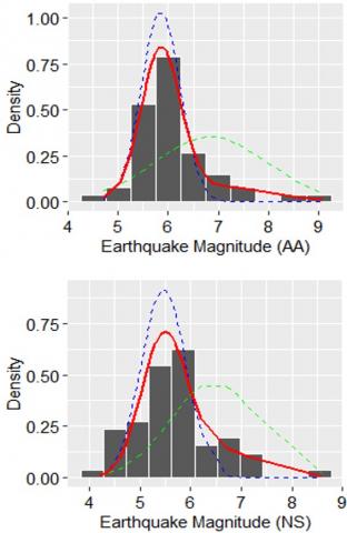
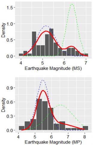
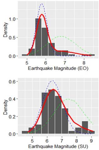
The summary of each component with its number, parameter estimates of selected models, in addition to the chosen model mean-variance values and empirical data for each case studied, are shown in Table 6. The second and third columns of Table 6 describe the grouping of data based on the largest posterior probability values. Accordingly, for all segments and the Sumatra megathrust zone, two seismicity patterns are found, which we denote by 1-level corresponding to periods of a moderate earthquake and by 2-level corresponding to periods of a strong earthquake.
Next, we will focus the discussion of the other columns in Table 6 only on the Aceh Andaman segment to save space. Meanwhile, in other cases, it can be explained in the same way. To do so, let us consider the third through sixth columns of Table 6. The number of components having a 1-level seismicity pattern is 44 with a Gaussian distribution N1(5.85; 0.14) and the number of components having a 2-level seismicity pattern is 9 with a Gaussian distribution N2(6.82; 1.28) where the weights of the two Gaussian distributions are 0.75 and 0.25, respectively.
Subsequently, the mean and variance values between the selected model and the empirical data are relatively equal, as can be seen in the last four columns of Table 6. In other words, the two main statistical parameters (i.e., mean and variance values) from the empirical data can be estimated with precision by the selected model. In addition, the PDF curves of Ν1(5.85; 0.14), Ν2(6.82; 1.28), and the 2-group GMM are shown in Figure 2 with different colors, namely blue, green, and red, respectively.
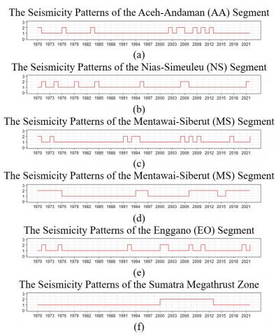
Accordingly, the seismicity patterns of the Aceh Andaman and Nias Simeulue segments are relatively more fluctuating compared to the other segments, as can be seen in Figure 3. We note that this condition is inseparable from two factors, that is, the values of a and b of these two segments are relatively larger compared to the other three segments (see Table 2), and there were two large earthquakes that occurred in a relatively close period in the Aceh Andaman (26/12/2004; Mw=9.10) and Nias Simeulue (28/03/2005; Mw=8.60).
Table 5. The results of normality and serial independence tests
|
Research Area |
Shapiro-Wilk Normality Test H0: The Data is Normally Distributed |
Ljung-Box Serial Independence Test H0: The Data is Serially Time-Independent |
||||||
|
W test |
p-value |
Decision of H0 |
$\hat{\boldsymbol{\rho}}(\boldsymbol{h})$ |
QLB |
p-value |
Decision of H0 |
||
|
Segments |
Aceh-Andaman (AA) |
0.860 |
1.083 × 10⁻⁵ |
Rejected |
0.137 |
7.930 |
0.160 |
Accepted |
|
Nias-Simeulue (NS) |
0.916 |
1.174 × 10⁻³ |
Rejected |
0.038 |
2.850 |
0.723 |
Accepted |
|
|
Mentawai-Siberut (MS) |
0.945 |
1.587 × 10⁻² |
Rejected |
0.042 |
0.669 |
0.985 |
Accepted |
|
|
Mentawai-Pagai (MP) |
0.897 |
2.478 × 10⁻⁴ |
Rejected |
0.432 |
18.504 |
0.002 |
Rejected |
|
|
Enggano (EO) |
0.825 |
2.005 × 10⁻⁶ |
Rejected |
0.148 |
5.643 |
0.343 |
Accepted |
|
|
Sumatra megathrust zone (SU) |
0.886 |
1.128 × 10⁻⁴ |
Rejected |
0.210 |
17.013 |
0.004 |
Rejected |
|
Table 6. The recapitulation of number of component (comp), parameter estimates of selected models, mean-variance values of the selected models and empirical data
| Research Area | Comp | Number of Comp | Parameters | Model | Empirical | ||||||
| δi | μi | $\sigma_i^2$ | Γ | Mean | Variance | Mean | Variance | ||||
| Segments | Aceh Andaman | 1 | 44 | 0.75 | 5.85 | 0.14 | n.a | 6.09 | 0.61 | 6.09 | 0.62 |
| (AA) | 2 | 9 | 0.25 | 6.82 | 1.28 | ||||||
| Nias Simeulue | 1 | 44 | 0.7 | 5.47 | 0.19 | n.a | 5.77 | 0.56 | 5.76 | 0.57 | |
| (NS) | 2 | 9 | 0.3 | 6.46 | 0.74 | ||||||
| Mentawai Siberut | 1 | 43 | 0.82 | 5.16 | 0.18 | n.a | 5.37 | 0.37 | 5.37 | 0.38 | |
| (MS) | 2 | 10 | 0.18 | 6.35 | 0.06 | ||||||
| Mentawai Pagai | 1 | 30 | 0.56 | 5.35 | 0.3 | $\left[\begin{array}{ll}0.87 & 0.13 \\ 0.15 & 0.85\end{array}\right]$ | 5.75 | 0.67 | 5.75 | 0.57 | |
| (MP) | 2 | 23 | 0.44 | 6.26 | 0.68 | ||||||
| Enggano | 1 | 44 | 0.76 | 5.78 | 0.08 | n.a | 6.02 | 0.38 | 6.03 | 0.39 | |
| (EO) | 2 | 9 | 0.24 | 6.8 | 0.56 | ||||||
| Sumatra megathrust zone (SU) | 40 | 0.74 | 6.35 | 0.43 | $\left[\begin{array}{ll}0.97 & 0.03 \\ 0.08 & 0.92\end{array}\right]$ | 6.64 | 0.81 | 6.64 | 0.64 | ||
| 2 | 13 | 0.26 | 7.47 | 0.98 | |||||||
Next, we discuss the seismicity patterns from a zonal analysis point of view. According to this, let us reconsider Tables 4 and 5. The model that fits the probability of empirical data (ePDF) is the 2-state GHMM, with a BIC value of 121.69. Thus, we conclude that the optimum level of seismic activity is two levels, with the presence of the Markov property in the sequence of seismic dynamics. Notice that the Markov properties of the seismic dynamics sequence are investigated based on the serial dependency test (with lag h=1) of the empirical data using the Ljung-Box test. As can be seen in Table 5, it is clear that “H0: The annual earthquake magnitude maximum in the Sumatra megathrust zone is serially time-independent” is rejected. Consequently, there was a one-year lag in the serial time dependency feature of the modeled data. This result conforms to the selected mixture models for the seismicity data in the Sumatra megathrust zone.
From the 2-state GHMM parameters determined, namely δi, μi, $\sigma_i^2$, and Γ, some aspects can be discussed. We obtain that the stationary distribution for two states is δi=(0.74, 0.26), with the Gaussian distribution parameters for each state being Ν1(6.35; 0.43) and Ν2(7.47; 0.98), respectively. This indicates that there is a 74% chance that the maximum earthquake magnitude will occur in a year that is far enough away from 2022 to be considered in a “strong state”, while the remaining 26% are in a “major state”. Additionally, from the first row of the transition probability matrix (Γ), when seismicity is in a “strong state”, as we can see, it either stays in that state with a probability of 0.97 or it moves to a “major state” with a prediction of 0.03. Using the same method, the second row of the Γ can be explained.
Consider the last row of Figure 3, from a time-dependent perspective, the “strong state” was documented by the beginning of 1970, and so seismic behavior shifted from “strong state” to “major state” between 2000 and 2012. Subsequently, it remained in a “strong state” from 2013 to 2022, as illustrated in Figure 3(f).
From the results mentioned in the previous paragraphs, we can conclude that the seismic phenomena of the five segments studied have a response range that tends to be similar for maximum earthquakes. However, the seismic dynamics of each segment are different from each other. The seismic pattern in the Aceh Andaman and Nias Simeulue segments is more volatile than the other three segments. This condition occurred because of two large megathrust earthquakes that occurred relatively close together in the Aceh Andaman segment (December 26, 2004) and Nias Simeulue (March 28, 2005). Additionally, the earthquake productivity and relative distribution of small and large earthquakes in these two segments are higher than in the other three segments. Thus, we can propose that seismic risk mitigation strategies in the Sumatra subduction zone can be structured in two different designs adapted to the dynamics of the seismicity patterns.
Figure 3. The step plot of the seismicity patterns
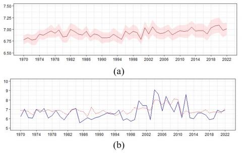
Figure 4. The maximum earthquake magnitude from 1970-2022 in the Sumatra megathrust zone: (a) The plot of a 95% confidence interval of simulations of 2-state GHMM; (b) The plots of observations (blue solid line) and simulations (red dotted line) of the annual maximum earthquake magnitudes
To get simulated yearly maximum earthquake magnitude data, a bootstrap sample of size 100 is generated using the 2-state GHMM. The resulting sample of parameters then produced the 95% confidence intervals that are displayed in Figure 4(a). Subsequently, we also provided a visualization of the plot of observations and simulations for the annual earthquake magnitude maximum data in the Sumatra megathrust, as can be seen in Figure 4(b). The vertical axis in Figure 4 is associated with the magnitude of earthquakes, while the horizontal axis is the time period (in years).
The relevance of our results to other studies can be presented as follows: As mentioned in the introduction, Orfanogiannaki et al. [6] and Rizal et al. [12] have provided the seismicity patterns in the Sumatra megathrust zone using PHMM, where the number of seismicity levels for each segment studied is two to four categories. Meanwhile, in this study, the number of seismicity levels for each subregion is limited to two categories. However, from the seismic pattern dynamics perspective, our results are in line with their findings, that is, the dynamics of seismic patterns in the Aceh Andaman and Nias Simeuleu segments fluctuate more than the remaining three segments of the megathrust zone in Sumatra.
The research area of the present study is the Sumatra megathrust zone, that has historically experienced frequent earthquakes, some of these have resulted in a significant number of deaths and severe infrastructure damage. Therefore, a comprehensive study of earthquake risk management through seismic modelling and pattern recognition in the research area has become a critical issue must be addressed.
We have successfully implemented two kinds mixture models of Gaussian distribution, namely G-group Gaussian independent mixture models (G-group GMMs) and N-state Gaussian hidden Markov models (N-state GHMMs), to determine seismicity patterns in the Sumatra megathrust zone, which contains five major earthquake sources, i.e., the Aceh-Andaman, Nias-Simeulue, Mentawai-Siberut, Mentawai-Pagai, and Enggano segments. In this study, the analysis is carried out from segmentally and zonally points of view.
Two results are obtained as follows. Firstly, from a segment analysis point of view, the results showed that the fluctuate of seismic patterns in the five segments is two levels due to the ePDF for those regions fits to Gaussian mixture model with two peaks, that is, the 2-group GMM for the Aceh-Andaman, Nias-Simeulue, Mentawai-Siberut, and Enggano segments, whereas the 2-state GHMM for the Mentawai-Pagai segment. The number of groups or states represents the earthquake magnitude scales, namely moderate and strong categories. Furthermore, we found that the seismic patterns of the Aceh-Andaman and Nias-Simeulue segments are more fluctuating than those of other segments. These conditions are inseparable from two factors, namely (1) two large megathrust earthquakes that was occurred in the Aceh-Andaman (December 26, 2004; with Mw=9.10) and Nias-Simeulue (March 28, 2005; with Mw=8.60) segments, and (2) the earthquake productivity and the relative distribution of small and large earthquakes in these two segments are relatively larger compared to the other three segments. Secondly, from a zonal analysis point of view, the appropriate probabilistic mixture model for the ePDF global modeled data is the 2-state GHMM. As a result, there were only two seismic levels: the moderate and strong categories. Moreover, the sequence of seismic patterns has the Markov property due to the modeled data had serial temporal dependence, which was present with a one-year lag.
We hope that these findings can improve seismic risk management, specifically for the area’s vulnerability to destructive earthquakes in the Sumatra megathrust zone, encompassing five seismic segments. The reason is that the model that we propose can not only recognize the pattern of a series of observations but can also be used to predict earthquake events in the future. Thus, we can say that there is an opportunity to integrate our results with early warning systems for earthquakes or urban planning on the coast of the Sumatra megathrust zone. However, in this current paper, we have not done this due to three limitations of this research: the observation range for modeled seismic data is relatively short for earthquake prediction studies; no investigations regarding the errors of the chosen models have been conducted; and the research assumptions still do not accurately reflect the ideal conditions of the seismicity phenomenon under study. As a future research direction, some limitations of this work that were mentioned in the previous paragraph can be worked out by researchers to improve this research.
The paper was funded by the Faculty of Mathematics and Natural Sciences (FMIPA), University of Bengkulu under the scheme of Penelitian Kerjasama Perguruan Tinggi (Grant No.: 1998/UN30.12/HK/2023).
[1] Bayona, V.J.A., von Specht, S., Strader, A., Hainzl, S., Cotton, F., Schorlemmer, D. (2019). A regionalized seismicity model for subduction zones based on geodetic strain rates, geomechanical parameters, and earthquake-catalog data. Bulletin of the Seismological Society of America, 109(5): 2036-2049. https://doi.org/10.1785/0120190034
[2] Huang, Q. (2006). Search for reliable precursors: A case study of the seismic quiescence of the 2000 western Tottori prefecture earthquake. Journal of Geophysical Research: Solid Earth, 111(B4). https://doi.org/10.1029/2005JB003982
[3] Ogata, Y. (1999). Seismicity analysis through point-process modeling: A review. In seismicity Patterns, Their Statistical Significance and Physical Meaning, pp. 471-507. https://doi.org/10.1007/s000240050275
[4] Rundle, J.B., Klein, W., Tiampo, K., Gross, S. (2000). Linear pattern dynamics in nonlinear threshold systems. Physical Review E, 61(3): 2418. https://doi.org/10.1103/PhysRevE.61.2418
[5] Kawamura, M., Chen, C.C., Wu, Y.M. (2014). Seismicity change revealed by ETAS, PI, and Z-value methods: A case study of the 2013 Nantou, Taiwan earthquake. Tectonophysics, 634: 139-155. http://doi.org/10.1016/j.tecto.2014.07.028
[6] Orfanogiannaki, K., Karlis, D., Papadopoulos, G.A. (2010). Identifying seismicity levels via Poisson hidden Markov models. Pure Appl Geophys, 167(8-9): 919-931. https://doi.org/10.1007/s00024-010-0088-y
[7] Votsi, I., Limnios, N., Tsaklidis, G., Papadimitriou, E. (2013). Hidden Markov models revealing the stress field underlying the earthquake generation. Physica A: Statistical Mechanics and its Applications, 392(13): 2868-2885. https://doi.org/10.1016/j.physa.2012.12.043
[8] Orfanogiannaki, K., Karlis, D., Papadopoulos, G.A. (2014). Identification of temporal patterns in the seismicity of Sumatra using Poisson Hidden Markov models. Research in Geophysics, 4(1). https://doi.org/10.4081/rg.2014.4969
[9] Hallo, M., Oprsal, I., Eisner, L., Ali, M.Y. (2014). Prediction of magnitude of the largest potentially induced seismic event. Journal of Seismology, 18(3): 421-431. http://doi.org/10.1007/s10950-014-9417-4
[10] Ünal, S., Çelebioğlu S., Özmen, B. (2014). Seismic hazard assessment of Turkey by statistical approaches. Turkish Journal of Earth Sciences, 23(3): 350-360. https://doi.org/10.3906/yer-1212-9
[11] Yip, C.F., Ng, W.L., Yau, C.Y. (2018). A hidden Markov model for earthquake prediction. Stochastic Environmental Research and Risk Assessment, 32(5): 1415-1434. https://doi.org/10.1007/s00477-017-1457-1
[12] Rizal, J., Gunawan, A. Y., Indratno, S. W., Meilano, I. (2018). Identifying dynamic changes in megathrust segmentation via poisson mixture model. In Journal of Physics: Conference Series, 1097(1): 012083. https://doi.org/10.1088/1742-6596/1097/1/012083
[13] Rizal, J., Gunawan, A. Y., Indratno, S. W., Meilano, I. (2021). The application of copula continuous extension technique for bivariate discrete data: A case study on dependence modeling of seismicity data. Mathematical Modelling of Engineering Problems, 8(5): 793-804. https://doi.org/10.18280/mmep.080516
[14] Rizal, J., Gunawan, A. Y., Indratno, S. W., Meilano, I. (2023). Seismic activity analysis of five major earthquake source segments in the Sumatra megathrust zone: Each segment and two adjacent segments points of view. Bulletin of the New Zealand Society for Earthquake Engineering, 56(2): 55-70. https://doi.org/10.5459/bnzsee.1555
[15] Mignan, A., King, G., Bowman, D., Lacassin, R., Dmowska, R. (2006). Seismic activity in the Sumatra–Java region prior to the December 26, 2004 (Mw=9.0–9.3) and March 28, 2005 (Mw=8.7) earthquakes. Earth and Planetary Science Letters, 244(3-4): 639-654. https://doi.org/10.1016/j.epsl.2006.01.058
[16] Dasgupta, S., Mukhopadhyay, B., Bhattacharya, A. (2007). Seismicity pattern in north Sumatra-Great Nicobar region: In Search of Precursor for the 26 December 2004 Earthquake. Journal of Earth System Science, 116(3): 215-223. https://doi.org/10.1007/s12040-007-0021-7
[17] Dewey, J.W., Choy, G., Presgrave, B., Sipkin, S., Tarr, A.C., Benz, H., Earle, P., Wald, D. (2007). Seismicity associated with the Sumatra–Andaman Islands earthquake of 26 December 2004. Bulletin of the Seismological Society of America, 97(1A): S25-S42. https://doi.org/10.1785/0120050626
[18] Denuit, M., Lambert, P. (2005). Constraints on concordance measures in bivariate discrete data. Journal of Multivariate Analysis, 93(1): 40-57. https://doi.org/10.1016/j.jmva.2004.01.004
[19] Somers, R.H. (1962). A new asymmetric measure of association for ordinal variables. American Sociological Review, 27(6): 799-811. https://doi.org/10.2307/2090408
[20] Tsapanos, T.M., Christova, C.V. (2000). Some preliminary results of a worldwide seismicity estimation: a case study of seismic hazard evaluation in South America. Annals of Geophysics, 43(1). https://doi.org/10.4401/ag-3618
[21] Tsapanos, T. M. (2001). Evaluation of the seismic hazard parameters for selected regions of the world: the maximum regional magnitude. Annali di Geofisica, 44(1). https://doi.org/10.4401/ag-3615
[22] Irsyam, M., Cummins, P.R., Asrurifak, M., Faizal, L., Natawidjaja, D.H., Widiyantoro, S., Meilano, I., Triyoso, W., Rudiyanto, A., Hidayati, S., Ridwan, M., Hanifa, N.R., Syahbana, A.J. (2020). Development of the 2017 national seismic hazard maps of Indonesia. Earthquake Spectra, 36: 112-136. https://doi.org/10.1177/8755293020951206
[23] Patel, E., Kushwaha, D.S. (2020). Clustering cloud workloads: K-means vs gaussian mixture model. Procedia Computer Science, 171: 158-167. https://doi.org/10.1016/j.procs.2020.04.017
[24] Nicolas, P., Bize, L., Muri, F., Hoebeke, M., Rodolphe, F., Ehrlich, S.D., Bessières, P. (2002). Mining Bacillus subtilis chromosome heterogeneities using hidden Markov models. Nucleic Acids Research, 30(6): 1418-1426. https://doi.org/10.1093/nar/30.6.1418
[25] Louvrier, J., Chambert, T., Marboutin, E., Gimenez, O. (2018). Accounting for misidentification and heterogeneity in occupancy studies using hidden Markov models. Ecological Modelling, 387: 61-69. https://doi.org/10.1016/j.ecolmodel.2018.09.002
[26] Dempster, A.P., Laird, N.M., Rubin, D.B. (1977). Maximum likelihood from incomplete data via the EM algorithm. Journal of the Royal Statistical Society: Series B (Methodological), 39(1): 1-22. https://doi.org/10.1111/j.2517-6161.1977.tb01600.x
[27] Lanjewar, R.B., Mathurkar, S., Patel, N. (2015). Implementation and comparison of speech emotion recognition system using Gaussian Mixture Model (GMM) and K-Nearest Neighbor (K-NN) techniques. Procedia Computer Science, 49: 50-57. https://doi.org/10.1016/j.procs.2015.04.226
[28] Medasani, S., Krishnapuram, R. (1999). A comparison of Gaussian and Pearson mixture modeling for pattern recognition and computer vision applications. Pattern Recognition Letters, 20(3): 305-313. https://doi.org/10.1016/S0167-8655(98)00149-4
[29] Proust, C., Jacqmin-Gadda, H. (2005). Estimation of linear mixed models with a mixture of distribution for the random effects. Computer Methods and Programs in Biomedicine, 78(2): 165-173. https://doi.org/10.1016/j.cmpb.2004.12.004
[30] Jain, A.K., Duin, R.P.W., Mao, J. (2000). Statistical pattern recognition: A review. IEEE Transactions on Pattern Analysis and Machine Intelligence, 22(1): 4-37. https://doi.org/10.1109/34.824819
[31] Kadirioğlu, F.T., Kartal, R.F. (2016). The new empirical magnitude conversion relations using an improved earthquake catalogue for Turkey and its near vicinity (1900-2012). Turkish Journal of Earth Sciences, 25(4): 300-310. https://doi.org/10.3906/yer-1511-7
[32] Sieh, K. (2007). The Sunda megathrust—past, present and future. Journal of Earthquake and Tsunami, 1(1): 1-19. https://doi.org/10.1142/S179343110700002X
[33] Duda, S.J., Nuttli, O.W. (1974). Earthquake magnitude scales. Geophysical Surveys, 1: 429-458. https://doi.org/10.1007/BF01452248
[34] Zucchini, W., MacDonald, I.L., Langrock, R. (2017). Hidden Markov Models for Time Series: An Introduction Using R. eBook ISBN 9781315372488, Chapman and Hall/CRC. https://doi.org/10.1201/b20790-2
[35] Jordan, M.I. (2004). Graphical models. Statistical Science, 19(1): 140-155. https://doi.org/10.1214/088342304000000026
[36] Schwarz, G. (1978). Estimating the dimension of a model. The Annals of Statistics, 461-464. https://doi.org/10.1214/aos/1176344136
[37] Rydelek, P.A., Sacks, I.S. (1989). Testing the completeness of earthquake catalogues and the hypothesis of self-similarity. Nature, 337(6204): 251-253. https://doi.org/10.1038/337251a0
[38] Woessner, J., Wiemer, S. (2005). Assessing the quality of earthquake catalogues: Estimating the magnitude of completeness and its uncertainty. Bulletin of the Seismological Society of America, 95(2): 684-698. https://doi.org/10.1785/0120040007
[39] Kvaerna, T., Ringdal, F. (1999). Seismic threshold monitoring for continuous assessment of global detection capability. Bulletin of the Seismological Society of America, 89(4): 946-959. https://doi.org/10.1785/BSSA0890040946
[40] Schorlemmer, D., Woessner, J. (2008). Probability of detecting an earthquake. Bulletin of the Seismological Society of America, 98(5): 2103-2117. https://doi.org/10.1785/0120070105
[41] Taramasco, O., Bauer, S. (2013). RHmm: Discrete, univariate or multivariate gaussian, mixture of univariate or multivariate gaussian HMM functions for simulation and estimation. Available at: https://citeseerx.ist.psu.edu/document?repid=rep1&type=pdf&doi=d78e5e65e74266b49e3467f42a7ec52d1b776952.
[42] Scrucca, L., Fop, M., Murphy, T.B., Raftery, A.E. (2016). mclust 5: Clustering, classification and density estimation using gaussian finite mixture models. The R Journal, 8(1): 289. https://doi.org/10.32614/RJ-2016-021
[43] Shapiro, S.S., Wilk, M.B., Chen, H.J. (1968). A comparative study of various tests for normality. Journal of the American Statistical Association, 63(324): 1343-1372. https://doi.org/10.1080/01621459.1968.10480932
[44] Ljung, G.M., Box, G.E. (1978). On a measure of lack of fit in time series models. Biometrika, 65(2): 297-303. https://doi.org/10.1093/biomet/65.2.297