Ahlam Alghanmi![]()
© 2024 The author. This article is published by IIETA and is licensed under the CC BY 4.0 license (http://creativecommons.org/licenses/by/4.0/).
OPEN ACCESS
The COVID-19 pandemic, which originated in 2019, has caused a significant global number of fatalities. The economic and healthcare impacts of COVID-19 infection in survivors have become evident during this period. An important first step towards the effective management of COVID-19 is an effective screening of patients, which includes radiology examinations using chest radiography as one of the primary screening modalities. Early research has shown that patients with pneumonia and COVID-19 infection show different anomalies in chest radiography images. Classifying images of COVID-19 and pneumonia diseases has proven to be a challenging task for computers. Several classification systems were developed using different databases in order to determine the category to which the detected image belongs. The accuracy percentage was assessed using these systems. However, there are instances where the imaging techniques may produce distorted images, low contrast images, or fail to accurately depict the edges of the internal organs. These challenges can have an impact on the accuracy of a classification model's design. In this study, a new robust model called FPD-VGG-16 is introduced. This model combines the Visual Geometry Group (VGG-16) deep learning technique with the Fractional Partial Differential (FrPDA) mathematical method. The idea of using FrPDA is to improve edges, increase the visibility of texture details, and retain smooth areas in comparison to using only deep algorithms. The proposed model demonstrates accurate pneumonia detection and COVID-19 classification from chest X-ray images; the model recorded an impressive accuracy of 98.1%, along with equally remarkable precision and recall values 0.982 and 0.980 respectively, as well as and f1-score score of 0.981. While 96.2% as an accuracy measure is achieved in this study without using the FrPDA algorithm.
COVID-19, fractional partial differential algorithms, image classification, image normalization, pneumonia infection, VGG-16
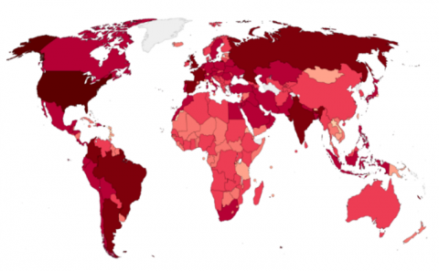
In early December 2019, there were reports of several patients in Wuhan City, China, who had pneumonia with unknown causes [1]. Some patients have exhibited severe acute respiratory syndrome (SARS) during the initial phases of this pneumonia, which has an unknown cause. However, it is important to note that only a small percentage of patients have exhibited symptoms of a rapid escalation in acute respiratory distress (ARD) disorder. Additionally, there have been reports of other worrisome complications as well. I'm sorry, but I need more context or information in order to provide a well-written response On January 7, 2020, the Chinese Centre for Disease Control and Prevention (CCDC) discovered a new strain of coronavirus (nCoV) from a throat swab sample collected from a patient in Wuhan. This virus was later designated as 2019-nCoV by the World Health Organisation (WHO) [2]. As of December 31, 2021, a global total of 284,992,606 cases of coronavirus infection have been reported, with 5,440,570 deaths and 252,735,264 recoveries [3]. The frontline experts used the real-time reverse transcription-polymerase chain reaction test as the first set for checking COVID-19 amid this tough time [4]. Reverse transcription method was applied to acquire the DNA from the individual infected. This DNA is subsequently subjected to PCR to amplify it before undergoing analysis. Hence, it is capable of detecting the coronavirus as this particular virus exclusively contains RNA patterns [5]. The results obtained from PCR kits for COVID-19 tests are currently being delayed due to increased demand. PCR kits are not considered reliable due to the presence of false-negative (FN) results [6]. Therefore, there is a need for alternative and robust diagnostic methods that can detect outbreaks of COVID-19 and pneumonia diseases at an early stage. Figure 1 illustrates a heat map showcasing the distribution of COVID-19 epidemic deaths, which have affected millions of people worldwide.
Chest X-rays are effective and cost-efficient diagnostic techniques that can detect outbreaks of COVID-19 and pneumonia diseases at an early stage. However, due to the significant similarities between COVID-19, viral pneumonia, and tuberculosis, it presents a challenge for physicians to distinguish between them solely based on chest X-rays [7-9]. Numerous research studies have been conducted to classify cases as either COVID-19 or healthy [10], COVID-19 or pneumonia [11], or COVID-19 or Tuberculosis (TB) [12]. However, these studies lacked the ability to accurately make a clear distinction between these diseases using chest x-rays.
Figure 1. A heat map showcasing the distribution of COVID-19 over the worldwide [7]
Medical image classification is the act of image analysis and determination of its appropriate "category". This can be likened to a virtual machine designed to mimic human behavior. Classifying medical images has proven to be a challenging task for computers, despite its seemingly straightforward nature. Multiple classification systems were developed using various databases to determine the category to which the detected image belongs. These systems were then used to assess the accuracy percentage [13, 14].
In classification models for COVID-19 and pneumonia, the imaging techniques occasionally produce images that contain artefacts, exhibit low contrast, or fail to clearly depict the boundaries of the visceral organs. As a result, these challenges can impact the accuracy of a classification model's design [15]. Therefore, it is necessary to do some preprocessing such as resizing, normalisation, and augmentation on these types of medical images [16-18].
Mathematical algorithms, such as integral differentials and reference-based methods, have been used to classify medical images. However, these algorithms did not achieve the optimal resolution [19]. Fractional partial differential algorithms (FrPDAs) have been used as a new image processing technique in the medical sector. Fractional differentials, a theory of arbitrary order, bear similarities to integral differentials [20]. The use of fractional differentials in the processing of images has been found to improve edges, increase the visibility of texture details, and retain smooth areas in comparison to conventional integral differential methods [21].
The contrast and clarity of images that have undergone fractional differential processing are mostly enhanced. The conventional fractional differentials manage edges, textures, and smooth areas in an image by using the same fractional order even though this strategy has some drawbacks. It is possible to use higher fractional orders to efficiently improve edges, but they frequently overlook smooth sections and weak textures. Regarding the lower fractional orders, they can weaken the edges while preserving smooth sections and weaker textures. Therefore, achieving image enhancement in practice is challenging and to address these challenges, researchers have developed both conventional and enhanced fractional differential (FD) frameworks for usage in the processing of digital images [22, 23]. In earlier research [24], the application of adaptive fractional derivatives to solve image denoising issues was investigated. Sharma et al. [21] proposed the operator YiFeiPu-2, which has shown to have greater convergence and precision, as well as six fractional differential masks. The mentioned differential operators have fixed fractional orders determined by humans. Consequently, modifying the area features of the image would not optimise image enhancement.
Furthermore, numerous studies have classified COVID-19 and related conditions using Convolutional Neural Networks (CNN) [25], Recurrent Neural Network - Long Short Term Memory (RNN-LSTM) [26], Visual Geometry Group (VGG-16) [27]. VGG-16 is a highly regarded CNN model in the field of computer vision, widely recognised as one of the most effective models available. It is specifically designed for tasks involving classification and localization. The VGG-16 model is renowned for its utilisation of 16 layers with weights, making it one of the most highly regarded vision model architectures currently available. Like many other popular networks such as GoogleNet and AlexNet, there are several well-known networks in the field of computer vision [28].
This study introduces a new robust model called FPD-VGG-16, which combines a deep learning technique known as VGG-16 with a mathematical method known as Fractional Partial Differential (FrPDA). The proposed model accurately detects and classifies pneumonia and COVID-19 from chest X-ray images. Fractional differentiation has started to play a very important role in various image and signal processing research fields. In image processing, fractional calculus can be rather interesting to improve edges, increase the visibility of texture details, and retain smooth areas in comparison to using only deep algorithms, which led the proposed model to high accuracy while maintaining the model's training complexity.
The paper has been organized thus: the investigation of the previous works is presented in Section 2 while Section 3 of this study presents a comprehensive overview of both the fractional difference algorithm and the VGG-16 network. Furthermore, this section discusses the datasets that were utilized and the performance metrics used to evaluate the performance of the proposed model. In Section 4 of the paper, an in-depth discussion is presented regarding the experiments conducted and the subsequent comparisons made. Finally, in Section 5, the study’s conclusion is made.
A COVID-19 epidemic was observed in Kumar et al. [29]. Medical experts conducted an investigation into the symptoms of the illness, which included fever, cough, muscle pain, and fatigue. Permanent diseases are uncommon. Influenza can lead to chest discomfort. COVID-19 is transmitted through particles or aerosols that are released when an infected individual coughs, talks, or sneezes. COVID-19 is different. The spread of variants can be rapid and pose a significant danger when they give rise to abnormal individuals. The results indicate that abnormalities are increasing in severity. The rapid progress in computing technology has driven the wide adoption of digital image processing in medicine. This includes various techniques such as image segmentation and augmentation. Deep Learning (DL) technologies, such as CNN [30], are utilized in the field of medical image processing. DL models have been shown to enhance the accuracy and effectiveness of various tasks such as forecasting, testing, and categorizing.
Asif et al. [31] focused on digitally detecting COVID-19 pneumonia cases via analysis of X-ray images. The DL model effectively identifies the unique characteristics and effects of COVID-19, thereby enhancing its categorization capabilities. There were 864 cases of pneumonia, COVID-19, and normal X-rays. Despite being built on massive data, the system underwent pre-processing and enhancement. In their study, Qjidaa et al. [32] developed a clinical decision-support system specifically developed for the identification of COVID-19 patients based on chest X-rays. Analysis was conducted on 30% of the collection, which consists of three classes. The data from two streams was obtained in an inappropriate manner and underwent extensive processing.
A study investigated by Khasawneh et al. [33] in which they identified chest X-rays using CNN. The initial photographs were captured at King Abdullah University Hospital in Jordan. I am 63.15 years old. From a 31-month-old child to a 96-year-old individual. Clinics can cause harm. Data stores were employed for evaluation after the system underwent training and testing. The models used include CNN, Mobile Nets, and VGG-16. The models are overfitting the photographs and failing to generalise to additional details. The analysis of combined data showed a detection performance of 98.7%, which was slightly higher than the effectiveness of maximal techniques. The identification of COVID-19 was credited to Haiti et al. The images in the Ray dataset are resized to 80×80, resulting in a resolution of 6400 pixels. I would like assistance with resizing and vectorizing images. One way to address inequality is by utilising a dataset consisting of 135 images of normal patients and 135 images of patients diagnosed with COVID-19. COVID-19 is comprised of three groups: 135 individuals with drug-induced blood clots, 135 healthy individuals, and 135 patients receiving intensive treatment. T2-weighted MRIs are an effective diagnostic tool. I would like to request MRIs with dimensions of 80x80. The image vectors are focused on X-rays with a resolution of 1:6400. The categorization strategies were unsuccessful on all three datasets. The prototype involved a comparison of DL and ML algorithms.
Alhwaiti et al. [34] recommended utilising DL methods for the identification of COVID-19 cases in X-ray images. Since the release of COVID-19 in December 2019, there has been no publicly available scientific dataset. Hospitals are required to share data from multiple sources. CNN classifier, Google Net, ResNet18, and ResNet50 are examples of pre-trained models. Additionally, there is the option of using grid search. This approach has a global scope. The training at CNN has been modified. The upcoming features include ILR, L2 regularisation, momentum, and minibatch size. Estimates are made for precision, accuracy, sensitivity, and F1-score. The prototype's ability to predict COVID-19 occurrences from records was objectively evaluated using various performance indicators. The prototypes of GS and ResNet50 have achieved significant breakthroughs.
Abiyev et al. [35] are credited with creating COVID-19 and CNN. The procedures for image processing include analyzing normal pneumonia and X-ray image databases, splitting images into training set, testing set, and validation set, resizing images, extracting features, and resampling information. The error rate is determined by comparing the latest responses to the target classes. The error function and learning algorithm have a subsequent impact on CNN signals. Images can be categorized into four main groups: upcoming, scaling down, feature extraction, and picture restoration. The intended model is a subset of the network model that aims to identify whether X-rays indicate the presence of pneumonia, COVID-19, or a normal case. The learning algorithm updates the models of CNN.
Elshennawy and Ibrahim [36] have developed assays specifically designed for detecting viral chest infections, including COVID-19. The collection consists of 5,856 X-rays, both positive and negative. Children between the ages of 1 and 5 who have different health issues are involved. The files for training, validation, and testing. The image database accounts for 30% of the proposal testing. The training of the prototype included different ratios, such as 50:50, 60:40, 70:30, 80:20, and 90:10. They analyzed split ratios using an 80/20 training/testing dataset. The algorithm was trained using 5740 intercepts, over 20 epochs, with a 0.0001 learning rate. Later, a model based on CNN (Convolutional Neural Network) was able to accurately identify cases of viral pneumonia in X-ray images. The AlexNet model is composed of convolutional layers. Convolution, max pooling, and normalization are processes used in convolutional layers. The SoftMax function is applied to one of the two layers, resulting in their combination. A 70:30 ratio was found to be effective in categorization training. The specificity is 99.84% and the sensitivity is 98.59%.
This section covers the techniques and phases of the suggested methodology that will be used to achieve the main objectives of this study. The used datasets, as well as the experimental environment, have been indicated.
3.1 An overview of the modified FrPDA
Fractional calculus is a branch of mathematics that generalizes the standard definitions of integral and derivative operators in the same upper line as do fractional powers allow to generalize the concept of exponent for real numbers. Fractional differential equations have become more popular in recent years as a powerful and organized mathematical tool for investigating various phenomena in the fields of science and engineering. Research in fractional differential equations spans across multiple disciplines and finds applications in a wide range of fields. These include continuum mechanics fluid mechanics, control systems, circuit systems, heat transfer, elasticity, electric drives, signal analysis, quantum mechanics, biomathematics, biomedicine, and social systems, bioengineering [37, 38].
To date, a universally accepted formula for defining fractional calculus has not yet been developed. Different definitions of fractional calculus have been developed as a result of the thorough analysis of the issue from numerous angles by mathematicians. The three traditional definitions of fractional calculus are the R-L, Capotu, and G-L definitions [39]. For the processing of medical images, we used the G-L definition, as it is less complex and requires only one coefficient. First, second and third order derivatives of f(t) were obtained by means of the L’Hospital rule:
$f^{\prime}(r)=\lim _{g \rightarrow 0} \frac{f(r+h)-f(r)}{g}$ (1)
$f^{\prime \prime}(r)=\left[f^{\prime}(t)\right]^{\prime} \lim _{g \rightarrow 0} \frac{f(r+2 h)-2 f(r+h)+f(r)}{g^2}$ (2)
$f^{\prime \prime \prime}(r)=\left[f^{\prime \prime}(r)\right]^{\prime} \lim _{g \rightarrow 0} \frac{f(r+3 h)-3 f(r+2 h)+f(r)}{g^3}$ (3)
The n-th order derivative (denoted as n![]() N) of function f(r) is derived mathematically as follows:
N) of function f(r) is derived mathematically as follows:
$f^{(n)}(r)=\lim _{g \rightarrow 0} g^{-n} \sum_{j=0}^n(-1)^j\left(\begin{array}{l}n \\ j\end{array}\right) f(r-j g)$ (4)
The gamma function generates the fractional order, ranging from integer to fraction. The v-order FD of function f(t) is described as the derivative of order (n+1) on the interval [a, b], where function f(r) has (n+1)-order derivatives.
$a D_b^v f(r)=\lim _{g \rightarrow 0} r^{-v} \sum_{j=0}^{[(b-a) / r]}(-1)^j\left(\begin{array}{c}v \\ j\end{array}\right) f(r-h g)$ (5)
where, the integer part of $\frac{b-a}{r}$ is $\left[\frac{b-a}{r}\right]$ and $\left(\begin{array}{l}v \\ j\end{array}\right)=\frac{v^i}{f^{!}(v-j)^{!}}$is binomial coefficient.
3.2 An overview of VGG-16 networks
One of the most heavily used deep learning CNN for vision tasks is the VGG-16 network [40]. VGG-16 is actually a specific implementation of the regular VGG network, but the difference is that if has a total of 16 layers (3 fully linked & 13 convolutional layers). Yet, the VGG-16 network has a specific outline as architecture. Initially, the input to be received by a VGG-16 network is a 224×224 image, which was kept standard as a result of cropping a 224×224 section from the center of each image in the ImageNet dataset. The receptive field on VGG is 3×3 which is used by the convolution filter is the smallest. A 1×1 convolution filter is also used by VGG to linearly transform the input. Next, a distinct linear function is applied, which is known as Rectified Linear Unit Activation Function to return an identical response on the input; while on the other hand, it would be a zero output for negative inputs. As a result of the fact that AlexNet, could be a classic CNN architecture and a Local Response Normalisation increases the time taken for training and the amount of memory used, and on the other hand also, it is not used by the hidden layers of VGG: the activation function for the hidden layer VGG is ReLu. Following the Convolution Phases, additionally, a Pooling layer are appended, which is used to reduce the dimensionality of the feature map, and it is due to reasons to reduce the parameters amount present in feature maps. Hence, a pooling layer is necessary, considering there were increasing filters for 64, then 128, and 256, and in the posterior levels 512 filters. You may also mention the fact that the VGG is made up of three interconnected layers with the first two combining 4096 channels:
In the $l$-th layer, we will consider transforming its inputs $x^l$, which form an order 3 tensor $x^l \in \mathbb{R}^{H^l \times W^l \times D^l}$. Where $x^l$ is the i-th row and j-th column and k-th depth of $x^l$ (in other words of $x^l$ is an element ${x}_{i,j,k}$ of $x^l$ ), it'll be typically be useful for us to know the triplet index set $((\mathrm{i}, \mathrm{j}, \mathrm{k}))$; i.e., the triplet $\left(i^l, j^l, d^l\right)$ with $0 \leq i^l<H^l, 0 \leq j^l<W^l$, and $0 \leq d^l<D^l$ that locates this particular element in $x^l$. Later in VGG training we'll use a kind of "minibatch" strategy where $N>1$, and so $x^l$ will typically become an order 4 tensor in $\mathbb{R}^{H^l \times W^l \times D^l \times N}$ where $N$ is the mini-batch size. But, for seriously issues sometimes it can be helpful to consider $N=1$. It turns out that in essentially all uses of our output tensor variables, we'll also use the zero-based indexing convention, so that a size $H^{l+1} \times W^{l+1} \times D^{l+1}$ output tensor is indexed by the triplets $\left(i^{l+1}, j^{l+1}, d^{l+1}\right), 0 \leq i^{l+1}<H^{l+1}, 0 \leq j^{l+1}<W^{l+1}$, $0 \leq d^{l+1}<D^{l+1}$.
In the $l$-th layer, our goal will be to transform the input $x^l$ to an output $y$, where $y$ and $x^{l+1}$ will refer to the same object. Thus, we expect $y$ to be of size $H^{l+1} \times W^{l+1} \times D^{l+1}$ (in other words, when we say that $y$ is the output of the $l$-th layer, we mean that it's the input to the (1+1)-st layer). An element in our output $y$ will be indexed by a triplet $\left(i^{l+1}, j^{l+1}, d^{l+1}\right), 0 \leq i^{l+1}<H^{l+1}, 0 \leq j^{l+1}<W^{l+1}$, $0 \leq d^{l+1}<D^{l+1}$.
3.2.1 The ReLU layer
The input size in the ReLU layer remains unchanged, and xl and y have the same size. Additionally, there is no need for parameter learning. Sometimes, ReLU is considered a truncation that was performed separately for every component of the input:
$y_{i, j, d}=\max \left\{0, x_{i, j, d}^l\right\}$ (6)
where, $0 \leq i<H^l=H^{l+1}, 0 \leq j<W^l=W^{l+1}$, and $0 \leq d<D^l=D^{l+1}$.
From the above equation, it is obvious that:
$\frac{\mathrm{d} y_{i, j, d}}{\mathrm{~d} x_{i, j, d}^l}=\left[\left[x_{i, j, d}^l>0\right]\right]$ (7)
where, $\left[\left[x_{i, j, d}^l>0\right]\right]$ represents the indicator function (having a value of 1 or 0 if the argument is true or false respectively).
Hence,
$\left[\frac{\partial z}{\partial x^l}\right]_{i, j, d}=\left\{\begin{array}{cl}{\left[\frac{\partial z}{\partial y}\right]_{i, j, d}} & \text { if } \boldsymbol{x}_{i, j, d}^l>0 \\ 0 & \text { otherwise }\end{array}\right.$. (8)
Noting that $y$ is an alias for $x^{l+1}$.
Note that the max (0, x) function cannot be differentiated at x=0, hence, Eq. (4) is somehow theoretically problematic. Therefore, it is not suitable in practice and as such, ReLU is safe to use.
3.2.2 The convolution layers
Using the following assumptions:
An input to layer l in the convolutional layers is a tensor of order 3 having size $H^l \times W^l \times D^l$.
A kernel of convolution is again a tensor of order 3 and its size is H×W×Dl.
Overlapping of the kernel at spatial position (0, 0, 0) on the input tensor makes the kernel slide over the input tensor generating product of related elements at all Dl channels and adding up the HWDl products generates the result of convolution at the related spatial position; the kernel is moved to the bottom, left-to-right and alternated again to complete this process.
A simple case is considered in this section where no padding is used and the stride is 1 . Hence, we have $y$ (or $x^{1+1}$ ) in $\mathbb{R}^{H^{l+1} \times W^{l+1} \times D^{l+1}}$, with $H^{l+1}=H^l-\mathrm{H}+1, \quad W^{l+1}=W^l-\mathrm{W}+1$, and $D^{l+1}=\mathrm{D}$.
The mathematical expression of the convolution process is given thus:
$\begin{aligned} & y_{i^{l+1}}, j^{l+1}, d =\sum_{i=0}^H \sum_{j=0}^W \sum_{d^{l=0}}^{D^l} f_{i, j, d^l, d} \times x_{{i^{l+1}}+{i, j}^{l+1}}+j, d^l \\ & \end{aligned}$ (9)
A repeat of this equation is performed for all 0≤d≤D=Dl+1, as well as for any other spatial location $\left(i^{l+1}, j^{l+1}\right)$ that satisfies the condition $0 \leq i^{l+1}<\bar{H}^l-H+1=H^{l+1}, 0 \leq j^{l+1}<$ $W^l-W+1=W^{l+1}$. The notation $x_{i^{l+1}+i, j^{l+1}+j, d^l}$ in the equation describes the component of $x^l$ indexed by the triplet $\left(i^{l+1}+\mathrm{i}, j^{l+1}+\mathrm{j}, d^1\right)$.
Even though a bias term $b_d$ is often added to $y_{i^{l+1}, j^{l+1}, d}$, this term was omitted in this case for better presentation.
Let’s now consider a pooling layer where the input to the l-th layer is $x^l \in \mathbb{R}^{H^l \times W^l \times D^l}$. The pooling operation has no parameters, so it doesn’t need to worry about learn any w’s. So, the w’s are going to be 0, and in this layer what we need to specify is the shape of the pooling layer. So, in the architecture of a ConvNet the dimensionality of a volume goes through a series of changes and in the very end it is Ho×Wo×Do, where we C the depth dimension). Let’s say that the spatial extent of the pooling is H×W. More so, the pooling operates with a stride of S, where H divides Hl and W divides Wl, then the output of the pooling O(l) will be an order 3 tensor and the size will be Hl+1×Wl+1×Dl+1, with:
$H^{l+1}=\frac{H^l}{H}, W^{l+1}=\frac{W^l}{W}, D^{l+1}=D^l$ (10)
The operation of a pooling layer upon xl is independently channel-wise. The matrix with Hl×Wl elements in each channel is partitioned into Hl+1×Wl+1 sub-regions that cannot overlap, and the size of each of the sub-region is H×W. Then, a sub-region is mapped by the pooling operator into a single number.
Average pooling and max pooling are the two commonly used types of pooling operators. For the average pooling, a sub-region is mapped by the pooling operator to its average value while in the max pooling, a sub-region is mapped by the pooling operator to its maximum value.
Mathematically,
max:
$y_{{i^{l+1}}, j^{l+1}, d}=\max _{0 \leq i<H, 0 \leq j<W} x_{i^{l+1} \times H+i, j}^{l+1} \times W+j, d^{\prime}$ (11)
Average:
$y_{i^{l+1}, j^{l+1}, d} \frac{1}{H W} \sum_{0 \leq i<H, 0 \leq j<W} x_{i^{l+1} \times H+i, l^{l+1} \times W+i, d^{\prime}}^l$ (12)
where, $0 \leq i^{l+1}<H^{l+1}, 0 \leq j^{l+1}<W^{l+1}$, and $0 \leq d<D^{l+1}=D^l$.
As a local operator, forward computation of pooling is a straightforward task; hence, attention is given to the back propagation and discussion is only focused on max pooling; let’s revisit the indicator matrix. For this indicator matrix, all that needs to be encoded is: for every element in y, where does it come from in $x^l$. A triplet $\left(i^l, j^l, d^l\right)$ is needed to identify one component in the input $x^l$, while another triplet $\left(l^{l+1}, j^{l+1}, d^{l+1}\right)$ is needed to find one component in $y$. The output $y_{i^{l+1}, j^{l+1}, d^{l+1}}$ of the pooling process is derivable from $x_{i^l, j^l, d^l}$, if and only if:
i. They are in the same channel;
ii. The $\left(i^l, j^l\right)$-th spatial entry belongs to the $\left(i^{l+1}, j^{l+1}\right)$-th subregion;
iii. The $\left(i^l, j^l\right)$-th spatial entry is the largest one in that sub-region.
A translation of these conditions gives the following equations:
$\left|\frac{i^l}{H}\right|=i^{l+1},\left|\frac{j^l}{W}\right|=j^{l+1}$ (13)
$\begin{aligned} & x_{i^l, j^l, d^l} \geq y_{i+i^{l+1} \times H, j+j^{l+1} \times W, d^l} \\ & \forall 0 \leq i<H, 0 \leq j<W\end{aligned}$ (14)
where, the floor function is given as $[\cdot]$. In the vertical or horizontal planes, if the stride is not $H(W)$, Eq. (11) must accordingly be altered.
Consider a given triplet $\left(i^{l+1}, j^{l+1}, d^{+1+1}\right)$ where only one $\left(i^l, j^l\right.$, $d^l$) triplet can satisfy the whole of these conditions, the indicator matrix can then be defined as:
$S\left(\boldsymbol{x}^l\right) \in \mathbb{R}^{\left(H^{l+1} W^{l+1} D^{l+1}\right) \times\left(H^l W^l D^l\right)}$ (15)
where, $S$ a row is specified by one triplet of indexes $\left(i^{l+1}, j^{l+1}\right.$, $d^{l+1}$ ) while a column is specified by $\left(i^l, j^l, d^l\right)$. Collectively, both triplets identify one component in $S\left(x^l\right)$ and that element is set to 0 if Eqs. (10) to (12) are not satisfied simultaneously, and 1 if satisfied. One row and one column of $S\left(x^l\right)$ corresponds to one element in $y$ and one element in $x^l$, respectively.
Considering this indicator matrix, it applies that:
$\operatorname{vec}(\boldsymbol{y})=S\left(\boldsymbol{x}^l\right) \operatorname{vec}\left(\boldsymbol{x}^l\right)$ (16)
Then, it is obvious that:
$\frac{\partial \operatorname{vec}(\boldsymbol{y})}{\partial\left(\operatorname{vec}\left(\boldsymbol{x}^l\right)^T\right)}=S\left(\boldsymbol{x}^l\right), \frac{\partial z}{\partial\left(\operatorname{vec}\left(\boldsymbol{x}^l\right)^T\right)}=\frac{\partial z}{\partial\left(\operatorname{vec}(\boldsymbol{y})^T\right)} S\left(\boldsymbol{x}^l\right)$ (17)
and consequently,
$\frac{\partial z}{\partial \operatorname{vec}\left(x^l\right)}=S\left(x^l\right)^T \frac{\partial z}{\partial \operatorname{vec}(\boldsymbol{y})}$ (18)
$S\left(x^l\right)$ is highly sparse and its entry in every row is exactly one non-zero entry. Hence, the entire matrix is not going to be used in the computation, rather, the locations of those nonzero entries are to be recorded - there are only $H^{l+1} W^{l+1} D^{l+1}$ such entries in $S\left(x^l\right)$.
The meaning of these equations can be explained using a simple example. Assume a $2 \times 2$ max pooling with a stride value of 2; the spatial subregion for each given channel $d^l$ has 4 elements in the input, where $(i, j)=(0,0),(1,0),(0,1)$ and $(1$, $1)$;also assume that the largest element among all the elements is the one at spatial location $(0,1)$. Then, in the forward pass of the input, the indexed value by $\left(0,1, d^l\right)$, i.e., $x_{0,1, d^l}^l$, is going to be allocated to the element occupying the $\left(0,0, d^l\right)$-th position in the output (i.e., $y_{0,0, d^l}$ ).
It is expected that in $S\left(x^l\right)$ one column can only contain a maximum of one non-zero entry if the strides are H & W. In the considered case, the $S\left(x^l\right)$ columns indexed by (0, 0, dl), (1, 0, dl) & (1, 1, dl) are all 0 vectors. The (0, 1, dl) column only contains one non-zero entry and the row index of this entry is only determined by (0, 0, dl). Therefore, the back-propagation process will give:
$\left[\frac{\partial z}{\partial \operatorname{vec}\left(x^l\right)}\right]_{\left(0,1, d^l\right)}=\left[\frac{\partial z}{\partial \operatorname{vec}(y)}\right]_{\left(0,0, d^l\right)}$ (19)
$\left[\frac{\partial z}{\partial \operatorname{vec}\left(\boldsymbol{x}^l\right)}\right]_{\left(0,0, d^l\right)}=\left[\frac{\partial z}{\partial \operatorname{vec}\left(\boldsymbol{x}^l\right)}\right]_{\left(1,0, d^l\right)}=\left[\frac{\partial z}{\partial \operatorname{vec}\left(\boldsymbol{x}^l\right)}\right]_{\left(1,1, d^l\right)}=0$ (20)
But if the pooling strides are comparatively less than H in the y-axis and less than W in the x-axis, then, the largest element in most of the pooling sub-regions could be one element in the input tensor. Therefore, one column of S(xl) may have more than one non-zero entries. If the stride is 1 in both directions and a 2×2 max pooling is applied, the element 9 will become the largest entry in 2 different pooling sub-regions as follows: $\left[\begin{array}{ll}5 & 6 \\ 8 & 9\end{array}\right] \&\left[\begin{array}{ll}6 & 1 \\ 9 & 1\end{array}\right]$. Hence, there are 2 non-zero entries in the S(xl) column that corresponds to the element 9 (indexed by (2, 2, dl) in the input tensor), with row indexes corresponding to (il+1, jl+1, dl+1)=(1, 1, dl) & (1, 2, dl). Therefore, this example provides that:
$\left[\frac{\partial z}{\partial \operatorname{vec}\left(x^l\right)}\right]_{\left(2,2, d^l\right)}=\left[\frac{\partial z}{\partial \operatorname{vec}(y)}\right]_{\left(1,1, d^l\right)}+\left[\frac{\partial z}{\partial \operatorname{vec}(y)}\right]_{\left(1,2, d^l\right)}$ (21)
3.3 Proposed methodology
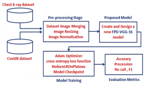
Image enhancement is a process that typically uses several algorithms to enhance the contrast and precise details of an image. The outcome of this research is going to be a new and effective model that will be FPD-VGG-16. The proposed model exhibits a high degree of accuracy in pneumonia and COVID-19 detection and classification using chest X-ray images. This goal will require the selection of a dataset appropriate for this activity before it can be achieved. To ensure the accurate identification of both pneumonia and COVID-19, two separate datasets are utilized in the new model. Each dataset corresponds to a specific disease infection and consists of Chest X-ray data. Figure 2 illustrates the acquisition of two separate datasets: a pneumonia dataset and a COVID-19 dataset. Both datasets undergo a data pre-processing stage to prepare them for input into the proposed FPD-VGG-16 model. Once the PD-VGG-16 model is created, it is trained using pre-processed data to learn how to accurately identify COVID-19 and Pneumonia. Following that, the FPD-VGG-16 network undergoes testing using new data to assess its effectiveness in accurately classifying the infection.
Figure 2. General diagram of the proposed FPD-VGG-16 classification model
3.3.1 Datasets description
Two different datasets were chosen for this study, particularly one for Pneumonia and one for COVID-19. The Dataset containing Pneumonia images is actually called the "Chest X-ray" dataset, and it was obtained from the Mendeley Data repository, comprising 5856 images in total [41]. Chest X-ray datasets normally contain two types/classes of data, namely the normal class (NC) and the pneumonia class (PC), where each class contains several images that are partitioned into training, testing, and validation sets. The NC category contains 1341 training images, 8 validation images, and 234 testing images, whereas the PC contains 3875 training images, 8 validation images, and 390 testing images.
On the one hand, the pictures in the “CovidX” dataset were utilized to train the FPD-VGG-16 model in detecting and classifying cases of COVID-19 infection from chest X-ray images. The CovidX dataset has 1300 images or 13975 chest x-ray images. These images assist in identifying whether the diagnosis of COVID-19 is accurate. This dataset is one of the most extensive chest X-ray datasets for diagnosing COVID-19, and it is publicly available. The CovidX data is compiled from five data sets, all of which are publicly available [42]. Table 1 shows the summary of the distribution of the selected datasets.
Table 1. The distribution of data in the chosen datasets
|
Dataset Name |
Training Data |
Validation Data |
Testing Data |
Total |
|
|
Chest X-ray |
Normal Class |
1341 |
8 |
234 |
5856 |
|
Pneumonia Class |
3875 |
8 |
390 |
||
|
CovidX |
|
13975 |
|||
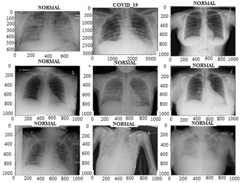
Furthermore, Figure 3 displays a compilation of chest X-ray images retrieved from selected databases. It demonstrates both normal chest X-ray images and a sample of a diseased chest X-ray, specifically from the COVID-19 class.
3.3.2 Data pre-processing
There are three main stages applied in these current studies before the implementation of any machine learning or deep learning model, and the first one is data pre-processing, and this is the most vital stage that must be conducted. The programmer should ensure that the data collected has a high quality to implement the model during the pre-processing.
The first pre-processing step is the merging of the two datasets (Chest X-ray and COVIDX). The merging took place by appending the datasets and assigning labels to each image. Thus, the merged dataset would contain three labels: Normal, COVID-19, and Pneumonia. The following equation represents the merging procedure. Eq. (22) illustrates this action.
merged dataset $=$ pneumonia dataset + COVIDx dataset (22)
The second step involves resizing the images in order to achieve an identical dimension for all of them. The chosen size is 224×224 pixels. Image resizing is necessary because if the images have different sizes, it can have a negative impact on the performance of the deep learning model. Image resizing ensures that the inputs are consistent. Eq. (23) represents the procedure for image resizing.
resized image $=\operatorname{resize}($ image,$(224,224))$ (23)
The final step involves data Normalization, which is necessary to ensure that the pixel values are within an equivalent range. During the normalization step, it is standard practise to ensure that the pixel values of the data have a mean value of zero and a standard deviation of one. Eq. (24) represents the normalization step.
normalized image $=($ image - mean $) /$ standard deviation (24)
After the pre-processing procedure is finished, the data is ready to be fed to the model for training.
Figure 3. Samples from the datasets showing normal and diseased X-rays
3.3.3 Training environment
The training of the model was done using the Adam Optimizer [43] and the categorical cross-entropy loss function [44]. During the training process of the model, recall, precision, accuracy, and F1-score are used as performance metrics to evaluate performance. In addition, callbacks like Model Check point [45], Early Stopping [46], and ReduceLROnPlateau [47] functions are employed to mitigate the issue of overfitting. The purpose of Model Check point is to save the model with the highest performance achieved during training. The Early Stopping function is responsible for continuously monitoring the training accuracy. If the accuracy does not show improvement over a specified number of epochs, the training process is halted. The ReduceLROnPlateau function is responsible for decreasing the learning rate if there is no improvement in accuracy after certain numbers of epoch.
In this scenario, the patience parameter is set to 1. This means that if the accuracy does not improve after 1 epoch, the learning rate will decrease. Furthermore, the stop patience parameter is set to 3, indicating that the training will halt if the accuracy does not improve after 3 epochs. The factor parameter is now set to 0.5, which indicates a decline in the learning rate by a factor of 0.5 if there is no improvement observed after one epoch.
This section discusses the achieved results using the datasets that were used, and also mentions the evaluation metrics.
4.1 Equations
The performance evaluation of the proposed model is based on the testing dataset outcomes. Some metrics are available to measure the model performance, which includes precision, recall, F1 score, and accuracy. Recall measures the model’s capability to identify all positive instances and is denoted as sensitivity. It estimates the number of correct positive classifications against the total number of true positive classifications. A high recall value implies low false-negative rates. In comparison, precision is the fraction of positive classifications which are correct. The number of true positive classifications divides the sum of true positive and false positive classifications. Precision is a measure of positive classification accuracy which has a high rate of false-positive. f-measure is also known as F1 score defined as the weighted harmonic mean of the precision and recall. It is a single number between 0 and 1 which does not capture the tradeoff one measure against the other. A high F1 score means you have a low false positive and low false negative; it has effectively reduced the cases of both types of error at the same time. That is, an F1 score may be a more useful measure when the VDR holds more importance than the false positive or false negative. Meanwhile, the accuracy is the ratio of the number of correct results to the total number of cases examined. It is most suitable where the entire data carries the same weight.
The values of these metrics, whether they are considered 'good' or 'bad', depend on the specific context and application of the model. In certain situations, there may be instances where precision holds greater significance than recall, or conversely, where recall is more important than precision. The objective is to attain an equilibrium between these metrics in order to achieve the best possible performance for the model. Comprehending each of these metrics is essential for gaining a comprehensive understanding of the model's performance.
Recall $=\frac{T P}{T P+F N}$ (25)
Precision $=\frac{T P}{T P+F P}$ (26)
F-Measure=2 Precision Recall Precision + Recall (27)
Accuracy $=\frac{T N+T P}{T N+T P+F N+F P}$ (28)
where, TP=true positive; FP=false positive; TN=true negative; FN=false negative.
4.2 Experimental outcomes
Based on the results that have been obtained, it can be argued that the proposed FPD-VGG-16 model is an extremely reliable model for the automatic identification of pneumonia and COVID-19 cases in chest X-ray images. Performance was measured through training and testing before finally using the model. This part will first discuss the results that have been obtained then compare the model’s performance with that of other similar works. Evaluation is very crucial in the training phase to ensure the functionality of the model and make changes where applicable.
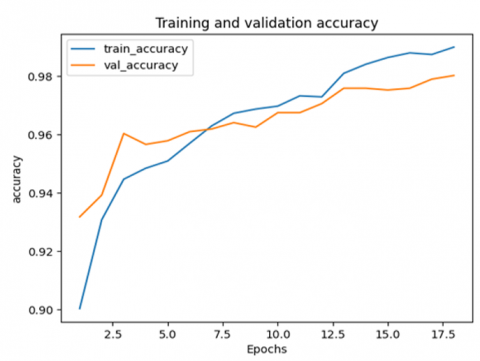
Figure 4. The achievement of the training and validation accuracy metric
Figure 4 shows the variation of the accuracy on the training and validation datasets, where the accuracy starts increasing rapidly after 2.5 epochs and reaches its maximum at 0.98 after 17 epochs.
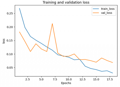
Figure 5 illustrates how the loss changes during training and validation steps. Throughout validation, the loss starts decreasing yet achieves a small peak between 6 and 7.5 epochs before reaching 0.08. On the other hand, the loss during training decreases gradually until it reaches 0.05 after approximately 17 epochs.
Figure 5. The achievement of the training and validation loss metric
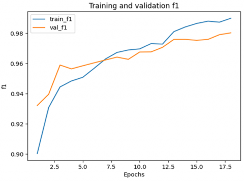
Figure 6. The achievement of the training and validation F1 metric
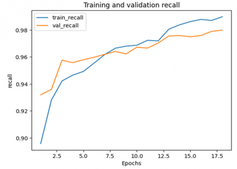
Figure 7. The achievement of the training and validation recall metric
The variation of the F1-value is illustrated in Figure 6. In both training and validation, the F1 score starts its gradual increase and reaches its maximum after 17 epochs. Ultimately, the achieved F1 score in training is larger than that in validation.
Figure 7 depicts that the recall in both training and validation starts increasing gradually as the number of epochs increases to 17.
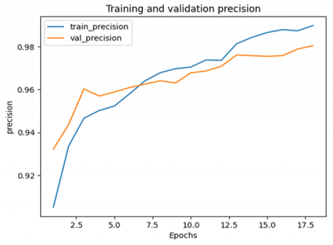
Figure 8. Achievement of the training and validation precision metric
Figure 8 illustrates that the precision value increases in the training and validation steps to reach its maximum at 17 epochs.
On the other hand, the precise metric values that were achieved during testing are summarized in Table 2. As illustrated, the proposed FPD-VGG-16 model achieved high scores for precision, recall, accuracy, and F1. More specifically, the achieved accuracy was 98.1%, the F1-score was 0.981, precision was 0.982, and recall was 0.980. The superior results can be attributed to the use of VGG16, a leading model in the field, which effectively distinguished between the three types. This underscores the model’s robustness and precision in classification tasks.
Table 2. Performance metric during testing
|
Metric |
Accuracy |
F1-score |
Recall |
Precision |
|
Value |
98.1% |
0.981 |
0.980 |
0.982 |
4.3 Comparative study
FPD-VGG-16 model was chosen for the present study because of its excellent features as well as its potential for good classification findings. However, there have been several studies that have utilized DL models to classify both pneumonia and COVID-19. Two studies are summarized, comparing their performances to those of the proposed FPD-VGG-16 model. The first published article on the use of VGG model [28] monitored accuracy at different stages: during training, validation, and testing. The recorded values for these stages were 97.13%, 96.48%, and 96.89%, respectively. Regarding the specific results for each class, the accuracy achieved for COVID-19 was 97.67%, for the normal class it was 97.93%, and for bacterial pneumonia it was 98.19%. The results demonstrated that utilizing VGG-16 can be a highly effective approach for accurately classifying cases of pneumonia and COVID-19.
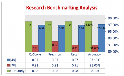
The second study that used DL model [48] employed a CNN architecture and utilized pre-trained VGG-16 and DenseNet121 models. In this scenario, the CNN model outperformed the pre-trained networks in terms of precision, recall, and F1-score. Additionally, the CNN model exhibited a significantly higher accuracy rate of 91% compared to the pre-trained networks' accuracy rate of 88%. When comparing the utilized VGG-16 model in this study to the two mentioned studies, Figure 8 demonstrates that the suggested model recorded the highest accuracy level of 98.10%. Figure 9 illustrates a comparison analysis in terms of accuracy, precision, recall and f1 of references [28, 48] and the proposed FPD-VGG-16 model.
Figure 9. A comparison analysis in terms of accuracy of references [28, 48] and the proposed FPD-VGG-16 model
Following the COVID-19 epidemic and the detrimental health impacts it caused, it was critical to quickly and readily identify COVID-19 infections. As the knowledge of COVID-19 expanded, it became crucial to differentiate it from pneumonia, as each of these diseases necessitates distinct healthcare measures. Consequently, numerous studies have been conducted to develop models capable of differentiating normal cases from pneumonia and COVID-19 cases. In this work, an FPD-VGG-16 model was hybridized with a mathematical framework to create an FPD-VGG-16 model. The objective was to classify cases into three categories: pneumonia, COVID-19, and normal. The proposed model underwent comprehensive training, and the subsequent testing demonstrated its ability to perform classification with exceptional precision (0.982) and a high level of accuracy (98.1%). This feature has the potential to be very useful for diagnosing COVID-19 and pneumonia illnesses. Alternatively, clinicians can use this model to check the accuracy of their diagnosis by comparing it to the suggested model.
Due to the dependency of many DL, as well as other AI methods, on training data, mainly on multiple types of medical data, such as both clinical data and medical images, abnormally large-scale training data is either unavailable or not available. The recognition that is the toughest part to detect and recognize the optimal models for the purpose of diagnosing COVID-19 due to the lack of access to an adequate amount of data. Further research is needed to rectify this situation. There is also the need for a benchmark dataset for COVID-19 diagnosis.
Since the arrival of the COVID-19 virus, several variants have emerged as a result of mutations. Collecting data for various COVID-19 variants within a limited timeframe is a challenging task, and there is consistently a lack of up-to-date datasets specifically related to COVID-19. To address this issue, it is necessary to implement a comprehensive and efficient data gathering strategy. Additionally, it is important to note that modifying the variant could potentially impact the effectiveness of a model that was trained using a different variant in the past. Therefore, further research is necessary.
In fact, COVID-19 samples contain fewer CTs, MRIs, and X-rays than pneumonia infection samples and healthy participant samples. This can be carried out using data augmentation, a technique weightlifting for generating new image samples by changing existing samples, such as flipping, rotating, zooming, or building noise in the complete images. Further study should be done to address criminal liability. Additionally, a definitive study identified the value of using imbalanced datasets. Data balancing is required in an upstream manner when it comes to dealing with imbalanced datasets. Finally, the efficiencies of provided models are compared before and after data balancing. Meanwhile, various individual types of data are available and may be combined, including demographics, MRI, X-ray, CT images, sound/auditory data, as well as clinical, laboratory, and blood test data. However, for the purpose of various studies related to COVID-19, it is required to combine several types of datasets and include organised and unstructured data on one level to execute further investigations.
[1] Lu, H., Stratton, C.W., Tang, Y.W. (2020). Outbreak of pneumonia of unknown etiology in Wuhan, China: The mystery and the miracle. Journal of Medical Virology, 92(4): 401. https://doi.org/10.1002%2Fjmv.25678
[2] Malik, H., Anees, T., Din, M., Naeem, A. (2023). CDC_Net: Multi-classification convolutional neural network model for detection of COVID-19, pneumothorax, pneumonia, lung Cancer, and tuberculosis using chest X-rays. Multimedia Tools and Applications, 82(9): 13855-13880. https://doi.org/10.1007/s11042-022-13843-7
[3] Zhang, J., Xie, Y., Li, Y., Shen, C., Xia, Y. (2020). COVID-19 screening on chest x-ray images using deep learning based anomaly detection. arXiv preprint arXiv:2003.12338, 27(10.48550).
[4] Tahamtan, A., Ardebili, A. (2020). Real-time RT-PCR in COVID-19 detection: Issues affecting the results. Expert Review of Molecular Diagnostics, 20(5): 453-454. https://doi.org/10.1080/14737159.2020.1757437
[5] Corman, V.M., Landt, O., Kaiser, M., et al. (2020). Detection of 2019 novel coronavirus (2019-nCoV) by real-time RT-PCR. Eurosurveillance, 25(3): 2000045. https://doi.org/10.2807/1560-7917.ES.2020.25.3.2000045
[6] Ayan, E., Ünver, H.M. (2019). Diagnosis of pneumonia from chest X-ray images using deep learning. In 2019 Scientific Meeting on Electrical-Electronics & Biomedical Engineering and Computer Science (EBBT), pp. 1-5. https://doi.org/10.1109/EBBT.2019.8741582
[7] Allen, J., Almukhtar, S., Aufrichtig, A., Barnard, A., Bloch, M., Cahalan, S., Yourishl, K. (2021). Coronavirus world map: Tracking the global outbreak. The New York Times, 22.
[8] Chow, E.J., Uyeki, T.M., Chu, H.Y. (2023). The effects of the COVID-19 pandemic on community respiratory virus activity. Nature Reviews Microbiology, 21(3): 195-210. https://doi.org/10.1038/s41579-022-00807-9
[9] Ioannidis, J.P. (2022). The end of the COVID‐19 pandemic. European Journal of Clinical Investigation, 52(6): e13782. https://doi.org/10.1111/eci.13782
[10] Ravichandran, B.D., Keikhosrokiani, P. (2023). Classification of COVID-19 misinformation on social media based on neuro-fuzzy and neural network: A systematic review. Neural Computing and Applications, 35(1): 699-717. https://doi.org/10.1007/s00521-022-07797-y
[11] Ibrahim, A.U., Ozsoz, M., Serte, S., Al-Turjman, F., Yakoi, P.S. (2021). Pneumonia classification using deep learning from chest X-ray images during COVID-19. Cognitive Computation, 1-13. https://doi.org/10.1007/s12559-020-09787-5
[12] Mahbub, M.K., Zamil, M.Z.H., Miah, M.A.M., Ghose, P., Biswas, M., Santosh, K.C. (2022). Mobapp4infectiousdisease: Classify COVID-19, pneumonia, and tuberculosis. In 2022 IEEE 35th International Symposium on Computer-Based Medical Systems (CBMS), Shenzen, China, pp. 119-124. https://doi.org/10.1109/CBMS55023.2022.00028
[13] Azizi, S., Mustafa, B., Ryan, F., Beaver, Z., Freyberg, J., Deaton, J., Loh, A., Karthikesalingam, A., Kornblith, S., Chen, T., Natarajan, V., Norouzi, M. (2021). Big self-supervised models advance medical image classification. In Proceedings of the IEEE/CVF International Conference on Computer Vision, Montreal, QC, Canada, pp. 3478-3488. https://doi.org/10.1109/ICCV48922.2021.00346
[14] Naser, Z.S., Khalid, H.N., Ahmed, A.S., Taha, M.S., Hashim, M.M. (2023). Artificial neural network-based fingerprint classification and recognition. Revue d'Intelligence Artificielle, 37(1): 129-137. https://doi.org/10.18280/ria.370116
[15] Ghosh, S.K., Ghosh, A. (2022). ENResNet: A novel residual neural network for chest X-ray enhancement based COVID-19 detection. Biomedical Signal Processing and Control, 72: 103286. https://doi.org/10.1016/j.bspc.2021.103286
[16] Wu, Q., Li, D., Yan, M., Li, Y. (2022). Mental health status of medical staff in Xinjiang Province of China based on the normalisation of COVID-19 epidemic prevention and control. International Journal of Disaster Risk Reduction, 74: 102928. https://doi.org/10.1016/j.ijdrr.2022.102928
[17] Elgendi, M., Nasir, M.U., Tang, Q., Smith, D., Grenier, J.P., Batte, C., Spieler, B., Leslie, W.D., Menon, C., Fletcher, R.R., Howard, N., Ward, R., Parker, W., Nicolaou, S. (2021). The effectiveness of image augmentation in deep learning networks for detecting COVID-19: A geometric transformation perspective. Frontiers in Medicine, 8: 629134. https://doi.org/10.3389/fmed.2021.629134
[18] Yaseen, N.A., Hadad, A.A.A., Taha, M.S. (2021). An anomaly detection model using principal component analysis technique for medical wireless sensor networks. In 2021 International Conference on Data Science and Its Applications (ICoDSA), Bandung, Indonesia, pp. 66-71. https://doi.org/10.1109/ICoDSA53588.2021.9617547
[19] Ibrahim, R.W., Jalab, H.A., Karim, F.K., Alabdulkreem, E., Ayub, M.N. (2022). A medical image enhancement based on generalized class of fractional partial differential equations. Quantitative Imaging in Medicine and Surgery, 12(1): 172-183. https://doi.org/10.21037%2Fqims-21-15
[20] Xu, L., Huang, G., Chen, Q.L., Qin, H.Y., Men, T., Pu, Y.F. (2020). An improved method for image denoising based on fractional-order integration. Frontiers of Information Technology & Electronic Engineering, 21(10): 1485-1493. https://doi.org/10.1631/FITEE.1900727
[21] Sharma, D., Chandra, S.K., Bajpai, M.K. (2019). Image enhancement using fractional partial differential equation. In 2019 Second International Conference on Advanced Computational and Communication Paradigms (ICACCP), Gangtok, India, Gangtok, India, pp. 1-6. https://doi.org/10.1109/ICACCP.2019.8882979
[22] Guo, X., Li, Y., Ling, H. (2016). LIME: Low-light image enhancement via illumination map estimation. IEEE Transactions on Image Processing, 26(2): 982-993. https://doi.org/10.1109/TIP.2016.2639450
[23] Roy, S., Shivakumara, P., Jalab, H.A., Ibrahim, R.W., Pal, U., Lu, T. (2016). Fractional Poisson enhancement model for text detection and recognition in video frames. Pattern Recognition, 52: 433-447. https://doi.org/10.1016/j.patcog.2015.10.011
[24] Al-Shamasneh, A.A.R., Jalab, H.A., Palaiahnakote, S., Obaidellah, U.H., Ibrahim, R.W., El-Melegy, M.T. (2018). A new local fractional entropy-based model for kidney MRI image enhancement. Entropy, 20(5): 344. https://doi.org/10.3390/e20050344
[25] Polsinelli, M., Cinque, L., Placidi, G. (2020). A light CNN for detecting COVID-19 from CT scans of the chest. Pattern Recognition Letters, 140: 95-100. https://doi.org/10.1016/j.patrec.2020.10.001
[26] Arantes Filho, L.R., Rodrigues, M.L., Rosa, R.R., Guimarães, L.N. (2022). Predicting COVID-19 cases in various scenarios using RNN-LSTM models aided by adaptive linear regression to identify data anomalies. Anais da Academia Brasileira de Ciências, 94: e20210921. https://doi.org/10.1590/0001-3765202220210921
[27] Alfaidi, A., Alshahrani, A., Aljohani, M. (2022). Artificial Intelligence-based Speech Signal for COVID-19 Diagnostics. In Proceedings of the 6th International Conference on Future Networks & Distributed Systems, Tashkent, TAS, Uzbekistan, pp. 311-317. https://doi.org/10.1145/3584202.3584247
[28] Karaddi, S.H., Srilakshmi, K., Sharma, L.D., Sharma, D., Singh, R.S. (2023). Detection of COVID-19 using CoviNet and VGG-16 Models. In 2023 3rd International conference on Artificial Intelligence and Signal Processing (AISP), VIJAYAWADA, India, pp. 1-5. https://doi.org/10.1109/AISP57993.2023.10134870
[29] Kumar, S.U., Kumar, D.T., Christopher, B.P., Doss, C.G.P. (2020). The rise and impact of COVID-19 in India. Frontiers in Medicine, 7: 250. https://doi.org/10.3389/fmed.2020.00250
[30] Sharma, N., Jain, V., Mishra, A. (2018). An analysis of convolutional neural networks for image classification. Procedia Computer Science, 132: 377-384. https://doi.org/10.1016/j.procs.2018.05.198
[31] Asif, S., Wenhui, Y., Jin, H., Jinhai, S. (2020). Classification of COVID-19 from chest X-ray images using deep convolutional neural network. In 2020 IEEE 6th International Conference on Computer and Communications (ICCC), Chengdu, China, pp. 426-433. https://doi.org/10.1109/ICCC51575.2020.9344870
[32] Qjidaa, M., Mechbal, Y., Ben-Fares, A., Amakdouf, H., Maaroufi, M., Alami, B., Qjidaa, H. (2020). Early detection of COVID19 by deep learning transfer Model for populations in isolated rural areas. In 2020 International Conference on Intelligent Systems and Computer Vision (ISCV), Fez, Morocco, pp. 1-5. https://doi.org/10.1109/ISCV49265.2020.9204099
[33] Khasawneh, N., Fraiwan, M., Fraiwan, L., Khassawneh, B., Ibnian, A. (2021). Detection of COVID-19 from chest x-ray images using deep convolutional neural networks. Sensors, 21(17): 5940. https://doi.org/10.3390/s21175940
[34] Alhwaiti, Y., Siddiqi, M.H., Alruwaili, M., Alrashdi, I., Alanazi, S., Jamal, M.H. (2021). Diagnosis of COVID-19 using a deep learning model in various radiology domains. Complexity, 2021: 1-10. https://doi.org/10.1155/2021/1296755
[35] Abiyev, R.H., Ismail, A. (2021). COVID-19 and pneumonia diagnosis in X-ray images using convolutional neural networks. Mathematical Problems in Engineering, 2021: 1-14. https://doi.org/10.1155/2021/3281135
[36] Elshennawy, N.M., Ibrahim, D.M. (2020). Deep-pneumonia framework using deep learning models based on chest X-ray images. Diagnostics, 10(9): 649. https://doi.org/10.3390/diagnostics10090649
[37] Li, B., Xie, W. (2015). Adaptive fractional differential approach and its application to medical image enhancement. Computers & Electrical Engineering, 45: 324-335. https://doi.org/10.1016/j.compeleceng.2015.02.013
[38] Zhang, Y., Yang, L., Li, Y. (2022). A novel adaptive fractional differential active contour image segmentation method. Fractal and Fractional, 6(10): 579. https://doi.org/10.3390/fractalfract6100579
[39] Teodoro, G.S., Machado, J.T., De Oliveira, E.C. (2019). A review of definitions of fractional derivatives and other operators. Journal of Computational Physics, 388: 195-208. https://doi.org/10.1016/j.jcp.2019.03.008
[40] Lorencin, I. (2022). Urinary bladder cancer diagnosis using customized vgg-16 architectures. Sarcoma, 10(11).
[41] Kermany, D., Zhang, K., Goldbaum, M. (2018). Large dataset of labeled optical coherence tomography (oct) and chest x-ray images. Mendeley Data, 3(10.17632).
[42] Hassan, E., Shams, M.Y., Hikal, N.A., Elmougy, S. (2023). COVID-19 diagnosis-based deep learning approaches for COVIDx dataset: A preliminary survey. Artificial Intelligence for Disease Diagnosis and Prognosis in Smart Healthcare, 107.
[43] Kingma, D.P., Ba, J. (2014). Adam: A method for stochastic optimization. arXiv preprint arXiv:1412.6980. https://arxiv.org/abs/1412.6980.
[44] Ho, Y., Wookey, S. (2019). The real-world-weight cross-entropy loss function: Modeling the costs of mislabeling. IEEE Access, 8: 4806-4813. https://doi.org/10.1109/ACCESS.2019.2962617
[45] Schmidt, F.D., Vulić, I., Glavaš, G. (2023). Free lunch: Robust cross-lingual transfer via model checkpoint averaging. arXiv preprint arXiv:2305.16834. https://arxiv.org/abs/2305.16834.
[46] Ferro, M.V., Mosquera, Y.D., Pena, F.J.R., Bilbao, V.M.D. (2023). Early stopping by correlating online indicators in neural networks. Neural Networks, 159: 109-124. https://doi.org/10.1016/j.neunet.2022.11.035
[47] Al-Kababji, A., Bensaali, F., Dakua, S.P. (2022). Scheduling techniques for liver segmentation: Reducelronplateau vs onecyclelr. In International Conference on Intelligent Systems and Pattern Recognition, pp. 204-212. https://doi.org/10.1007/978-3-031-08277-1_17
[48] Shinde, A.P. (2022). Multiclass classification of COVID-19, Tb, Pneumonia, and health cases using Deep Learning (Doctoral dissertation, Dublin, National College of Ireland). https://norma.ncirl.ie/id/eprint/6305.