Samira Faisal Abushilah![]() | Ayaat Maan Khalf*
| Ayaat Maan Khalf*![]()
© 2024 The authors. This article is published by IIETA and is licensed under the CC BY 4.0 license (http://creativecommons.org/licenses/by/4.0/).
OPEN ACCESS
One difficulty in using circular distribution is the existence of the modified Bessel function, $I_p(\kappa)$, which cannot be computed easily. In this paper, we consider the problem of calculating the solution of the ratio, $I_1(\kappa)\left(I_0(\kappa)\right)^{-1}$, to extract the value of the parameter $\kappa$, one of the parameters of the sine-model circular distribution. At first, a direct calculation is suggested in this paper to compute the solution of the ratio by using optimization approach with the nonlinear minimization (Newton-Raphson method). After that, to check whether the direct computation for the solution of the ratio is better than the function, $\operatorname{Al} \operatorname{inv}(\cdot)$, in R's circular package, or not, we consider a simulation study designed to compare the results of the function that we have suggested with the estimator $\operatorname{Al} \operatorname{inv}(\cdot)$. Also, we examine the difference between the true value of $\kappa$ and the estimated values using a t-test with level of significance $\alpha=0.05$ and we compare the estimated biases of the estimators with the approximation to the bias for the concentration parameter $\kappa$.
circular statistics, bivariate circular data, sine-model circular distribution, nonlinear optimization, modified Bessel function of the first kind
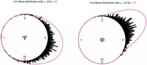
Circular statistics which are also called directional statistics is a branch of statistics specifically designed to deal with circular data. which is data that can be represented as points on the unit circle and these points can be represented by an angle on circumference of the circle, $\theta \in[0,2 \pi)$, or $\theta \in$ $(-\pi, \pi]$, or by the unit vector $(\cos \theta, \sin \theta)$ [1] (see Figure 1).
The aim of this study is to calculate the solution of the ratio $I_1(\kappa)\left(I_0(\kappa)\right)^{-1}$ which represent the modified Bessel function of the first kind and order one and zero, and the solution will be the value of the parameter $\kappa_i ; i=1,2$, one of the parameters of the sine-model circular distribution.
In the circular statistic, circular distributions are of interest in a wide range of fields, such as medicine [2] biology [3], geology [4], protein dihedral angles [5], political studies [6], image analysis [7]. One of the most important distributions is von-Mises distribution (see Figure 1). This distribution was introduced by von-Mises in 1918, and the probability density function for this distribution is defined by [7]:
$f(\theta ; \mu, \kappa)=\left(2 \pi I_0(\kappa)\right)^{-1} e^{\kappa \cos (\theta-\mu)}, 0 \leq \theta<2 \pi$, (1)
where, $\kappa$ is the concentration parameter such that $\kappa \geq 0, \mu$ is the circular mean and $I_0(\kappa)$ is the modified Bessel function of order zero [8], which is given by:
$I_p(\kappa)=\frac{1}{2 \pi} \int_0^{2 \pi} \cos (p \theta) e^{\kappa \cos \theta} d \theta, p=0,1,2, \ldots$ (2)
Mardia and Sutton [8] introduced the bivariate von-Mises with eight parameters before Rivest introduced a six-parameter version in 1988. For two circular random variables, $\vartheta_1$ and $\vartheta_2$, the probability density function of sine-model of the bivariate von-Mises distribution is given by [9-13]:
$f\left(\vartheta_1, \vartheta_2\right)=C_{\text {sine }} \exp \left\{\kappa_1 \cos \left(\vartheta_1-\mu_1\right)+\right.
\left.\kappa_2 \cos \left(\vartheta_2-\mu_2\right)+\delta \sin \left(\vartheta_1-\mu_1\right) \sin \left(\vartheta_2-\mu_2\right)\right\}$ (3)
for $0 \leq \vartheta_1, \vartheta_2 \leq 2 \pi, \kappa_1, \kappa_2 \geq 0,0 \leq \mu_1, \mu_2 \leq 2 \pi, C_{Sine }$ is a normalization constant which is defined by:
$C_{Sine }=\left[4 \pi^2 \sum_{i=0}^{\infty}\left(\begin{array}{c}2 r \\ r\end{array}\right)\left(\frac{\delta^2}{4 \kappa_1 \kappa_2}\right)^r I_i\left(\kappa_1\right) I_i\left(\kappa_2\right)\right]^{-1}$ (4)
One difficulty in using circular distribution is the existence of the modified Bessel function, $I_p(\kappa)$, which cannot be computed easily.
Therefore, in this paper, we consider the problem of calculating the solution of the function,
$M B(\kappa)=I_1(\kappa)\left(I_0(\kappa)\right)^{-1},$
which represents the modified Bessel function of first kind and order one and zero. A direct computation is explored for the solution of the function $M B(\kappa)$. At first, the optimization approach with the nonlinear minimization (Newton-Raphson method) is used under the maximum likelihood estimators with a specific assumption are used to calculate the solution of the ratio $I_1(\kappa)\left(I_0(\kappa)\right)^{-1}$ to reach the optimal solution.
We begin in Section 2, by given a direct computation for the solution of the ratio. In Section 3, simulation study is considered to evaluate the performance of the approach that we have suggested by using R' s circular package. The conclusion and the future of our research will be presented in Section 4.
Figure 1. von-Mises circular distribution under simulated data
The presence of the modified Bessel function, $I_m(\kappa)$, is one difficulty in using the Sine-Mosel circular distribution. In this section we introduce optimization approach with the nonlinear minimization (Newton-Raphson method) to calculate the inverse of the modified Bessel function for extraction the value of the parameter $\kappa_i ; i=1,2$, one of the parameters of sinemodel circular distribution.
Let $G_1=\left\{\left(\phi_{11}, \psi_{11}\right),\left(\phi_{12}, \psi_{12}\right), \ldots,\left(\phi_{1 n}, \psi_{1 n}\right)\right\}$ and $G_2=$ $\left\{\left(\phi_{21}, \psi_{21}\right),\left(\phi_{22}, \psi_{22}\right), \ldots,\left(\phi_{2 m}, \psi_{2 m}\right)\right\}$ be two independent random samples from sine-model circular distribution, $\operatorname{SBM}(\mu, \wedge)$ distribution, $\mu=\left(\begin{array}{l}\mu_1 \\ \mu_2\end{array}\right)$ and $\Lambda=\left(\begin{array}{cc}\kappa_1 & 0 \\ 0 & \kappa_2\end{array}\right)$, with the probability density function:
$\begin{gathered}f(\phi, \psi)=C_{Sine} \exp \left\{\kappa_1 \cos \left(\phi-\mu_1\right)+\kappa_2 \cos \left(\psi-\mu_2\right)\right. \\ \left.+\delta \sin \left(\phi-\mu_1\right) \sin \left(\psi-\mu_2\right)\right\}\end{gathered}$
The direct computation is constructed using the optimization approach with the nonlinear minimization function in R’s circular package, and the proposed algorithm is presented in Algorithm 1. In the R’s circular package, the nonlinear minimization caries out a minimization of any function (x) using a Newton-Raphson algorithm.
Newton-Raphson algorithm (NR), which is introduced by Isaac Newton and Joseph Raphson [4], is a method for finding a better approximation to the root of a continuous and differentiable real valued function. The Newton-Raphson method of one variable is implemented in the following way:
Assuming that the root for the function g(x) is near the point $x=x_n$, the NR algorithm tell us that a better approximation for the root is computed as follows:
$x_{n+1}=x_n-\frac{g\left(x_n\right)}{g^{\prime}\left(x_n\right)},$
where, $g^{\prime}\left(x_n\right)$ is the slope of the tangent line to the graph $g(x)$ at the point $x=x_n$. The process should be repeated many times by setting $x_n=x_{n+1}$ till $x_{n+1}$ close to $x_n$ in order to get the desired accuracy to get a better approximation, where $x_{n+1}$ is the best root approximate.
To show how the Newton-Raphson technique works let the function g(x) take the following formula:
$g(x)=x^2-4.$
In order to find the root of the function g(x) using the Newton-Rahson algorithm we need to determine starting point:
Let $\quad x_0=3 \rightarrow g\left(x_0\right)=5, \mathrm{~g}^{\prime}\left(x_0\right)=6 \rightarrow x_1=2.1667$ and $x_2=2.0789$, we repeat the process many times till the difference between successive approximations that is smaller than chosen tolerance.
Using the samples $\left\{\left(\phi_{11}, \psi_{11}\right),\left(\phi_{12}, \psi_{12}\right), \ldots,\left(\phi_{1 n}, \psi_{1 n}\right)\right\}$ and $\quad\left\{\left(\phi_{21}, \psi_{21}\right),\left(\phi_{22}, \psi_{22}\right), \ldots,\left(\phi_{2 m}, \psi_{2 m}\right)\right\} \quad$ a $\quad$ direct computation to compute the inverse of the function $M B(\kappa)$ under sine-model circular distribution with different concentration parameters is constructed as follows:
1. Calculate the MLE for the one-sample and two-sample sine-model circular distribution which is given by:
$R_{1 e \vartheta}=n^{-1}\left[\left(\sum_{i=1}^n \cos \left(\vartheta_i\right)\right)^2+\left(\sum_{i=1}^n \sin \left(\vartheta_i\right)\right)^2\right]^{0.5}$ (5)
$R_{2 e \vartheta}=\left[\left[S S_{\vartheta N}+C C_{\vartheta N}\right] / N ; \vartheta=\phi, \psi\right.$, (6)
where,
$S S_{\vartheta N}=\left[\left(\sum_{i=1}^n \cos \left(\vartheta_{1 i}\right)\right)^2+\left(\sum_{i=1}^n \sin \left(\vartheta_{1 i}\right)\right)^2\right]^{0.5}$,
$C C_{\vartheta N}=\left\lceil\left(\sum_{j=1}^m \cos \left(\vartheta_{2 j}\right)\right)^2+\left(\sum_{j=1}^m \sin \left(\vartheta_{2 j}\right)\right)^2\right]^{0.5}$.
2. Consider the starting point $\kappa_0$ for the concentration parameter such that $\kappa_0 \in[0, h], h>0$.
3. Apply optimization approach using the starting point $\kappa_0$ from Step (2) and the function $g_i\left(\kappa_i\right), f_i\left(\kappa_i\right)$ which is defined by:
$g_i\left(\kappa_i\right)=a b s\left[R_{1 e \vartheta}-I_1\left(\kappa_i\right) / I_0\left(\kappa_i\right)\right] ; i=1,2$
$f_i\left(\kappa_i\right)=a b s\left[R_{2 e \vartheta}-I_1\left(\kappa_i\right) / I_0\left(\kappa_i\right)\right] ; i=1,2$
where, $R_{1 e \vartheta}$ and $R_{2 e \vartheta}$ is the right hand side of Eqs. (5)-(6).
4. The result of the optimization approach will be the solution for the function:
$M B(\kappa)=I_1(\kappa)\left(I_0(\kappa)\right)^{-1}$.
This direct computation is constructed using the optimization approach with the non- linear minimization function in R’s circular package, and is presented in Algorithm 1.
|
Algorithm 1: Solution of the First Kind Modified Bessel Function |
|
Data: Circular data $\left\{\left(\phi_{11}, \psi_{11}\right), \ldots,\left(\phi_{1 n}, \psi_{1 n}\right)\right\}$, $\left\{\left(\phi_{21}, \psi_{21}\right), \ldots,\left(\phi_{2 m}, \psi_{2 m}\right)\right\}$ Result: Estimators $\widehat{\kappa_1}, \widehat{\kappa_2}$. begin $\operatorname{input}\left\{\mu_1, \mu_2, \kappa_1, \kappa_2, n, m, \kappa_0\right\}$ $N \leftarrow n+m$ for (i in 1: 1000) do Generate the data from BvM $\left(\left(\begin{array}{l}\mu_1 \\ \mu_2\end{array}\right),\left(\begin{array}{cc}\kappa_1 & 0 \\ 0 & \kappa_2\end{array}\right)\right)$ with the pdf $\begin{aligned} & C_{sine} \exp \left\{\kappa_1 \cos \left(\phi-\mu_1\right)+\kappa_2 \cos \left(\psi-\mu_2\right)+\delta \sin (\phi-\right. \\ & \left.\left.\mu_1\right) \sin \left(\psi-\mu_2\right)\right\}\end{aligned}$ Calculate $\begin{gathered}S S_{1 N} \leftarrow\left[\left(\sum_{i=1}^n \cos \left(\phi_{1 i}\right)\right)^2+\left(\sum_{i=1}^n \sin \left(\phi_{1 i}\right)\right)^2\right]^{0.5} \\ C C_{1 N} \leftarrow\left[\left(\sum_{i=1}^n \cos \left(\phi_{2 i}\right)\right)^2+\left(\sum_{i=1}^n \sin \left(\phi_{2 i}\right)\right)^2\right]^{0.5} \\ S S_{2 N} \longleftarrow\left[\left(\sum_{i=1}^n \cos \left(\psi_{1 i}\right)\right)^2+\left(\sum_{i=1}^n \sin \left(\psi_{1 i}\right)\right)^2\right]^{0.5} \\ C C_{2 N} \leftarrow\left[\left(\sum_{i=1}^n \cos \left(\psi_{2 i}\right)\right)^2+\left(\sum_{i=1}^n \sin \left(\psi_{2 i}\right)\right)^2\right]^{0.5} \\ \frac{I_1\left(\widehat{\kappa_1}\right)}{I_0\left(\widehat{\kappa}_1\right)}[i] \leftarrow\left[\left(S S_{1 N}+C C_{1 N}\right) / N\right] ; \frac{I_1\left(\widehat{\kappa_2}\right)}{I_0\left(\widehat{\kappa_2}\right)}[i] \leftarrow\left[\left(S S_{2 N}+\right.\right. \left.\left.C C_{2 N}\right) / N\right]\end{gathered}$ use Non-Linear Minimization $\left(f_1, \kappa_0\right)$ use Non-Linear Minimization $\left(f_2, \kappa_0\right)$ end begin Function $\left(\kappa_1\right)$ $f_1\left(\kappa_1\right)=a b s\left[R e_\phi-I_1\left(\kappa_1\right)\left(I_0\left(\kappa_1\right)\right)^{-1}\right]$ return $\left(f_1\left(\kappa_1\right)\right)$ end begin Function $\left(\kappa_2\right)$ $f_2\left(\kappa_2\right)=a b s\left[R e_\phi-I_1\left(\kappa_2\right)\left(I_0\left(\kappa_2\right)\right)^{-1}\right]$ return $\left(f_2\left(\kappa_2\right)\right)$ end calculate paired t-test 1. Test the null hypothesis $H_0: E\left(\widehat{\kappa_l}-\widehat{\kappa_{A_ l}}\right)=0$ against $H_1: E\left(\widehat{\kappa_l}-\widehat{\kappa_{A_l}}\right) \neq 0$ with level of significant $\alpha=0.05$ 2. The difference between the true value of $\kappa_i ; i=1,2$ and the estimations $\widehat{\kappa_l}, \widehat{\kappa_{A_l}}$ is tested using a t-test with $\alpha=0.05$ (i.e level of significant) end |
In the R’s circular package, the function NLM (Non-Linear Minimization) carries out a minimization of any function $g(x)$ using a Newton-Raphson algorithm, which has been described above. The NLM function which is a numerical function based on the Newton-Rahson algorithm, where the slope $g^{\prime}\left(x_n\right)$ may be numerically estimated. Sometimes it can diverge, but in practice, and during our research we have not noticed any such behaviour.
We consider a simulation study in this section to check whether the algorithm which has been presented in the previous section to compute the solution for the function $M B(\kappa)$ is better than the current function, $\mathrm{A} 1 \operatorname{inv}(\cdot)$, in $\mathrm{R}$ 's circular package, or not. We design the simulation to achieve several objectives. First, compare the results of the algorithm that we have suggested, the estimator $\hat{\kappa}_i$, with the estimator $\hat{\kappa}_A$ which is calculated using the following formula:
$\operatorname{A1inv}(x)=\left\{\begin{array}{c}2 x+x^3+\frac{5 x^5}{6}, 0 \leq x<0.53 \\ -0.4+1.39 x+\frac{0.43}{1-x}, 0.53 \leq x<0.85 \\ \frac{1}{3 x-4 x^2+x^3}, 0.85 \leq x\end{array}\right.$
Secondly, we have to examine the difference between the estimated value with the true value of $\kappa$. Thirdly, we calculate the biases for each estimator. Fourthly, we have to compare the estimated biases of the estimators $\hat{\kappa}_i$ and $\hat{\kappa}_{A_i}$ with the approximated to the bias of the MLE theoretically which is considered by Mardia and Jupp [7], which is given by.
$E\left[\hat{\kappa}_i-\kappa_i\right] \simeq \frac{3 \kappa_i}{n}$.
We show the results of the evaluation in Tables 1-4, Figures 2-5. It is interesting to know that with different values of κ the function that we have proposed has a good performance, while when the true value of κ is small the function A1inv(.) does not show a good performance. Also, we noticed that with different values of κ the results of these two functions are close to each other, also we noticed that:
1. Table 1 and Table 2 show that the results of the function that we have proposed are close to the true value under different values of $\kappa_1$ and $\kappa_2$ of the one-sample bivariate sine-model.
Table 1. Comparison between the true value and the estimated values of $\kappa_1$, and the approximated to the bias under, $n=500$ and $\mu=\left(\begin{array}{l}0 \\ 0\end{array}\right)$ of the one-sample bivariate sinemodel
|
True Parameters |
Estimated Parameters |
Approx. to Bias |
Estimated Bias |
||
|
$\kappa_1$ |
$\hat{k}_1$ |
$\widehat{k}_{\mathrm{A}_1}$ |
$\kappa_1$ |
$\hat{k}_1$ |
$\widehat{k}_{\mathrm{A}_1}$ |
|
0.2 |
0.211 |
0.211 |
0.001 |
0.011 |
0.011 |
|
0.4 |
0.407 |
0.41 |
0.002 |
0.007 |
0.001 |
|
0.6 |
0.605 |
0.605 |
0.004 |
0.005 |
0.005 |
|
0.8 |
0.804 |
0.803 |
0.005 |
0.004 |
0.003 |
|
1.0 |
1.005 |
1.001 |
0.006 |
0.005 |
0.001 |
|
1.2 |
1.203 |
1.195 |
0.007 |
0.003 |
-0.005 |
|
1.4 |
1.401 |
1.394 |
0.008 |
0.001 |
-0.006 |
|
1.6 |
1.605 |
1.598 |
0.010 |
0.005 |
0.002 |
|
1.7 |
1.703 |
1.696 |
0.010 |
0.003 |
-0.004 |
|
2.0 |
2.011 |
2.009 |
0.012 |
0.011 |
0.009 |
|
2.2 |
2.204 |
2.197 |
0.013 |
0.004 |
-0.003 |
|
2.6 |
2.599 |
2.592 |
0.016 |
-0.001 |
-0.008 |
|
3.1 |
3.097 |
3.083 |
0.019 |
-0.003 |
-0.017 |
|
3.6 |
3.607 |
3.580 |
0.022 |
0.007 |
-0.019 |
|
5.0 |
5.026 |
5.009 |
0.030 |
0.026 |
0.009 |
|
5.5 |
5.540 |
5.53 |
0.033 |
0.040 |
0.028 |
|
6.5 |
6.523 |
6.516 |
0.039 |
0.023 |
0.016 |
|
8.5 |
8.535 |
8.532 |
0.051 |
0.035 |
0.032 |
|
9.5 |
9.548 |
9.546 |
0.057 |
0.048 |
0.046 |
|
10 |
10.079 |
10.077 |
0.060 |
0.079 |
0.077 |
|
Mean Absolute Error |
0.01605 |
0.0151 |
|||
Table 2. Comparison between the true value and the estimated values $\kappa_2 \hat{\kappa}_2$, and the approximated to the bias $n=500$ and $\mu=\left(\begin{array}{l}0 \\ 0\end{array}\right)$ of the one-sample bivariate sine-model
|
True Parameters |
Estimated Parameters |
Approx. to Bias |
Estimated Bias |
||
|
$\kappa_2$ |
$\hat{k}_2$ |
$\widehat{k}_{\mathrm{A}_2}$ |
$\kappa_2$ |
$\hat{k}_2$ |
$\widehat{k}_{\mathrm{A}_2}$ |
|
0.25 |
0.259 |
0.259 |
0.002 |
0.009 |
0.009 |
|
0.50 |
0.503 |
0.503 |
0.003 |
0.003 |
0.003 |
|
0.75 |
0.753 |
0.753 |
0.005 |
0.003 |
0.003 |
|
1.00 |
1.006 |
1.002 |
0.006 |
0.006 |
0.002 |
|
1.25 |
1.256 |
1.249 |
0.008 |
0.006 |
-0.002 |
|
1.50 |
1.502 |
1.495 |
0.009 |
0.002 |
-0.005 |
|
1.75 |
1.755 |
1.748 |
0.011 |
0.005 |
-0.002 |
|
2.00 |
2.004 |
1.996 |
0.012 |
0.004 |
-0.004 |
|
2.25 |
2.252 |
2.245 |
0.014 |
0.002 |
-0.003 |
|
2.50 |
2.501 |
2.494 |
0.015 |
0.001 |
-0.006 |
|
3.00 |
3.027 |
3.015 |
0.018 |
0.027 |
0.015 |
|
3.50 |
3.518 |
3.494 |
0.021 |
0.018 |
-0.006 |
|
4.00 |
4.013 |
3.985 |
0.024 |
0.013 |
-0.015 |
|
4.50 |
4.506 |
4.504 |
0.027 |
0.006 |
0.004 |
|
6.00 |
6.039 |
6.029 |
0.036 |
0.039 |
0.029 |
|
7.00 |
7.039 |
7.033 |
0.042 |
0.039 |
0.033 |
|
8.00 |
8.047 |
8.043 |
0.048 |
0.047 |
0.043 |
|
9.00 |
9.054 |
9.051 |
0.054 |
0.054 |
0.050 |
|
10.0 |
10.066 |
10.064 |
0.060 |
0.066 |
0.064 |
|
Mean Absolute Error |
0.0184 |
0.01568 |
|||
2. Table 3 and Table 4 show that the results of the function that we have proposed are close to the true value under different values of $\kappa_1$ and $\kappa_2$ of the two-sample bivariate sinemodel.
3. The results of the paired t-test in Tables 5-8 indicate that for a variety of $\kappa$ values the suggested estimator and the classical estimator are significantly different since the p-values of the t-test are $<0.05$.
4. We noticed that the suggested function exhibits a good performance compared to the current function Alinv(.).
Table 3. Comparison between the true value and the estimated values of $\kappa_1$, and the approximated to the bias, $n=500$ and $\mu=\left(\begin{array}{l}0 \\ 0\end{array}\right)$ of the two-sample bivariate sine-model
|
True Parameters |
Estimated Parameters |
Approx. to Bias |
Estimated Bias |
||
|
$\kappa_1$ |
$\hat{k}_1$ |
$\hat{k}_{\mathrm{A}_1}$ |
$\kappa_1$ |
$\hat{k}_1$ |
$\hat{k}_{\mathrm{A}_1}$ |
|
0.2 |
0.209 |
0.209 |
0.001 |
0.009 |
0.009 |
|
0.4 |
0.405 |
0.405 |
0.002 |
0.005 |
0.005 |
|
0.6 |
0.607 |
0.607 |
0.004 |
0.007 |
0.007 |
|
0.8 |
0.806 |
0.805 |
0.005 |
0.006 |
0.005 |
|
1.0 |
1.003 |
0.999 |
0.006 |
0.003 |
-0.001 |
|
1.2 |
1.201 |
1.192 |
0.007 |
0.009 |
-0.008 |
|
1.4 |
1.402 |
1.396 |
0.008 |
0.002 |
-0.004 |
|
1.6 |
1.604 |
1.597 |
0.009 |
0.004 |
-0.003 |
|
1.7 |
1.702 |
1.695 |
0.010 |
0.002 |
-0.005 |
|
2.0 |
1.999 |
1.992 |
0.012 |
-0.008 |
-0.008 |
|
2.2 |
2.202 |
2.195 |
0.013 |
0.002 |
-0.005 |
|
2.6 |
2.603 |
2.596 |
0.016 |
0.003 |
-0.004 |
|
3.1 |
3.099 |
3.087 |
0.019 |
-0.001 |
-0.014 |
|
3.6 |
3.604 |
3.576 |
0.022 |
0.004 |
-0.024 |
|
5.0 |
5.007 |
4.991 |
0.030 |
0.007 |
-0.009 |
|
5.5 |
5.527 |
5.515 |
0.033 |
0.027 |
0.015 |
|
6.5 |
6.503 |
6.496 |
0.039 |
0.003 |
-0.004 |
|
8.5 |
8.535 |
8.531 |
0.051 |
0.035 |
0.031 |
|
9.5 |
9.527 |
9.525 |
0.057 |
0.027 |
0.025 |
|
10 |
10.036 |
10.034 |
0.060 |
0.036 |
0.034 |
|
Mean Absolute Error |
0.010 |
0.011 |
|||
Table 4. Comparison between the true value of the parameter and the estimated values of $\kappa_2$, and the approximated to the bias $\mathrm{s} n=500$ and $\mu=\left(\begin{array}{l}0 \\ 0\end{array}\right)$ of the two-sample bivariate sinemodel
|
True Parameters |
Estimated Parameters |
Approx. to Bias |
Estimated Bias |
||
|
$\kappa_2$ |
$\hat{k}_2$ |
$\hat{k}_{\mathrm{A}_2}$ |
$\kappa_2$ |
$\hat{k}_2$ |
$\hat{k}_{\mathrm{A}_2}$ |
|
0.25 |
0.259 |
0.259 |
0.002 |
0.009 |
0.009 |
|
0.50 |
0.504 |
0.504 |
0.003 |
0.004 |
0.004 |
|
0.75 |
0.752 |
0.751 |
0.005 |
0.002 |
0.001 |
|
1.00 |
1.004 |
1.000 |
0.006 |
0.004 |
0.000 |
|
1.25 |
1.254 |
1.246 |
0.008 |
0.004 |
-0.005 |
|
1.50 |
1.505 |
1.498 |
0.009 |
0.005 |
-0.002 |
|
1.75 |
1.752 |
1.745 |
0.011 |
0.002 |
-0.005 |
|
2.00 |
2.003 |
1.996 |
0.012 |
0.003 |
-0.004 |
|
2.25 |
2.251 |
2.244 |
0.014 |
0.001 |
-0.006 |
|
2.5 |
2.504 |
2.497 |
0.015 |
0.004 |
-0.003 |
|
3.00 |
3.006 |
2.994 |
0.018 |
0.006 |
-0.006 |
|
3.50 |
3.512 |
3.487 |
0.021 |
0.012 |
-0.013 |
|
4.00 |
4.006 |
3.978 |
0.024 |
0.006 |
-0.022 |
|
4.50 |
4.509 |
4.487 |
0.027 |
0.009 |
-0.013 |
|
6.00 |
6.038 |
6.029 |
0.036 |
0.038 |
0.029 |
|
7.00 |
7.018 |
7.018 |
0.042 |
0.018 |
0.018 |
|
8.00 |
8.019 |
8.015 |
0.048 |
0.019 |
0.015 |
|
9.00 |
9.013 |
9.011 |
0.054 |
0.013 |
0.011 |
|
10.0 |
10.042 |
10.040 |
0.060 |
0.042 |
0.040 |
|
11.0 |
11.057 |
11.056 |
0.066 |
0.057 |
0.056 |
|
Mean Absolute Error |
0.0129 |
0.0131 |
|||
Table 5. Paired t-test between the suggested function and the current function A1inv(.) and a t-test between the true value and the estimated values of $\kappa_1$ with level of significant $\alpha=$ 0.05 of the one-sample bivariate sine-model
|
$k_1$ |
$\widehat{\boldsymbol{\kappa}}_1$ |
p-Value of t-Test |
||
|
$\hat{\kappa}_1 \sim \hat{\kappa}_{A 1}$ |
$\kappa_1 \sim \hat{\kappa}_1$ |
$\kappa_1 \sim \hat{\kappa}_{A 2}$ |
||
|
0.2 |
0.211 |
<2.2×10⁻¹⁶ |
0.953 |
0.953 |
|
0.4 |
0.407 |
<2.2×10⁻¹⁶ |
0.291 |
0.192 |
|
0.6 |
0.605 |
<2.2×10⁻¹⁶ |
0.109 |
0.091 |
|
0.8 |
0.804 |
<2.2×10⁻¹⁶ |
0.624 |
0.900 |
|
1.0 |
1.005 |
<2.2×10⁻¹⁶ |
0.286 |
0.153 |
|
1.2 |
1.203 |
<2.2×10⁻¹⁶ |
0.101 |
0.177 |
|
1.4 |
1.401 |
<2.2×10⁻¹⁶ |
0.160 |
0.668 |
|
1.6 |
1.605 |
<2.2×10⁻¹⁶ |
0.874 |
0.511 |
|
1.7 |
1.703 |
<2.2×10⁻¹⁶ |
0.244 |
0.286 |
|
2.0 |
2.011 |
<2.2×10⁻¹⁶ |
0.212 |
0.498 |
|
2.2 |
2.204 |
<2.2×10⁻¹⁶ |
0.575 |
0.929 |
|
2.6 |
2.599 |
<2.2×10⁻¹⁶ |
0.367 |
0.574 |
|
3.1 |
3.097 |
<2.2×10⁻¹⁶ |
0.251 |
0.151 |
|
3.6 |
3.607 |
<2.2×10⁻¹⁶ |
0.458 |
0.209 |
|
5.0 |
5.026 |
<2.2×10⁻¹⁶ |
0.211 |
0.438 |
|
5.5 |
5.540 |
<2.2×10⁻¹⁶ |
0.344 |
0.436 |
|
6.5 |
6.523 |
<2.2×10⁻¹⁶ |
0.523 |
0.196 |
|
8.5 |
8.535 |
<2.2×10⁻¹⁶ |
0.223 |
0.311 |
|
9.5 |
9.548 |
<2.2×10⁻¹⁶ |
0.122 |
0.160 |
|
10 |
10.079 |
<2.2×10⁻¹⁶ |
0.206 |
0.251 |
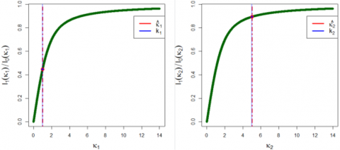
5. In Figure 2 and Figure 3, we can see that the values of the estimators $\hat{\kappa}_i$ and $\hat{\kappa}_{A_i}, \mathrm{i}=1,2$ are close to the true values of the concentration parameters under different one-sample bivariate sine-model.
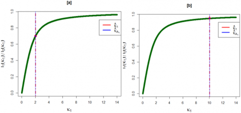
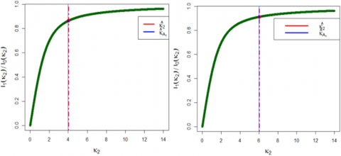
6. In Figure 4 and Figure 5, we can see that the values of the estimators $\hat{\kappa}_i$ and $\hat{\kappa}_{A_i}, \mathrm{i}=1,2$ are close to the true values of the concentration parameters under different two-sample bivariate sine-model.
7. In Figure 6, we can see that the estimated values $\hat{\kappa}_i$, i=1, 2 are so close to the true values of the concentration parameters under different parameters of the sine-models.
8. Compare the bias for each estimator $\hat{\kappa}_i$ and $\hat{\kappa}_{A_i}$ with the approximation of the bias we found that the bias for the proposed estimator $\hat{\kappa}_i$ is less than or equal to the approximated bias when the sample size is large.
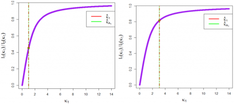
Figure 2. Comparison between the estimators, $\hat{\kappa}_1$ and $\hat{\kappa}_{A 1}$. The panels in this figure show $I_1(\kappa) / I_0(\kappa)$ (vertical axis) against the true value of the concentration parameter $\kappa_1$ (horizontal axis)
Figure 3. Comparison between the estimators, $\hat{\kappa}_2$ and $\hat{\kappa}_{A 2}$. The panels in this figure show $I_1(\kappa) / I_0(\kappa)$ (vertical axis) against the true value of the concentration parameter $\kappa_2$ (horizontal axis)
Figure 4. Comparison between the estimators, $\hat{\kappa}_1$ and $\hat{\kappa}_{A 1}$. The panels in this figure show $I_1(\kappa) / I_0(\kappa)$ (vertical axis) against the true value of the concentration parameter $\kappa_1$ (horizontal axis)
Figure 5. Comparison between the estimators, $\hat{\kappa}_2$ and $\hat{\kappa}_{A_2}$. The panels in this figure show $I_1(\kappa) / I_0(\kappa)$ (vertical axis) against the true value of the concentration parameter $\kappa_2$ (horizontal axis)
Figure 6. Comparison between the true value of the parameters $\kappa_i$ and the estimated values $\hat{\kappa}_i, \mathrm{i}=1,2$. The panels in this figure show $I_1(\kappa) / I_0(\kappa)$ (vertical axis) against the true value of the concentration parameter $\kappa_i$ (horizontal axis)
Table 6. Paired t-test between the suggested function and the current function A1inv(.) and a t-test between the true value and the estimated values of $\kappa_2$ with level of significant $\alpha=0.05$ of the one-sample bivariate sine-model
|
$k_2$ |
$\widehat{\boldsymbol{\kappa}}_2$ |
p-Value of t-Test |
||
|
$\hat{\kappa}_2 \sim \hat{\kappa}_{A 2}$ |
$\kappa_2 \sim \hat{\kappa}_2$ |
$\kappa_2 \sim \hat{\kappa}_{A 2}$ |
||
|
0.25 |
0.259 |
<2.2×10⁻¹⁶ |
0.681 |
0.681 |
|
0.50 |
0.503 |
<2.2×10⁻¹⁶ |
0.274 |
0.260 |
|
0.75 |
0.753 |
<2.2×10⁻¹⁶ |
0.175 |
0.295 |
|
1.00 |
1.006 |
<2.2×10⁻¹⁶ |
0.842 |
0.553 |
|
1.25 |
1.256 |
<2.2×10⁻¹⁶ |
0.233 |
0.140 |
|
1.50 |
1.502 |
<2.2×10⁻¹⁶ |
0.107 |
0.562 |
|
1.75 |
1.755 |
<2.2×10⁻¹⁶ |
0.280 |
0.927 |
|
2.00 |
2.004 |
<2.2×10⁻¹⁶ |
0.939 |
0.323 |
|
2.25 |
2.252 |
<2.2×10⁻¹⁶ |
0.132 |
0.450 |
|
2.50 |
2.501 |
<2.2×10⁻¹⁶ |
0.826 |
0.293 |
|
3.00 |
3.027 |
<2.2×10⁻¹⁶ |
0.345 |
0.549 |
|
3.50 |
3.518 |
<2.2×10⁻¹⁶ |
0.462 |
0.341 |
|
4.00 |
4.013 |
<2.2×10⁻¹⁶ |
0.975 |
0.156 |
|
4.50 |
4.506 |
<2.2×10⁻¹⁶ |
0.189 |
0.801 |
|
6.00 |
6.039 |
<2.2×10⁻¹⁶ |
0.725 |
0.986 |
|
7.00 |
7.039 |
<2.2×10⁻¹⁶ |
0.357 |
0.175 |
|
8.00 |
8.047 |
<2.2×10⁻¹⁶ |
0.483 |
0.661 |
|
9.00 |
9.054 |
<2.2×10⁻¹⁶ |
0.899 |
0.770 |
|
10.0 |
10.066 |
<2.2×10⁻¹⁶ |
0.268 |
0.321 |
Table 7. Paired t-test between the suggested function and the current function A1inv(.) and a t-test between the true value and the estimated values of $\kappa_1$ with level of significant $\alpha=$ 0.05 of the two-sample bivariate sine-model
|
$k_1$ |
$\widehat{\kappa}_1$ |
p-Value of t-Test |
||
|
$\hat{\kappa}_1 \sim \hat{\kappa}_{A 1}$ |
$\kappa_1 \sim \hat{\kappa}_1$ |
$\kappa_1 \sim \hat{\kappa}_{A 1}$ |
||
|
0.2 |
0.209 |
<2.2×10⁻¹⁶ |
0.833 |
0.834 |
|
0.4 |
0.405 |
<2.2×10⁻¹⁶ |
0.175 |
0.178 |
|
0.6 |
0.607 |
<2.2×10⁻¹⁶ |
0.150 |
0.183 |
|
0.8 |
0.806 |
<2.2×10⁻¹⁶ |
0.109 |
0.318 |
|
1.0 |
1.003 |
<2.2×10⁻¹⁶ |
0.232 |
0.534 |
|
1.2 |
1.201 |
<2.2×10⁻¹⁶ |
0.628 |
0.222 |
|
1.4 |
1.402 |
<2.2×10⁻¹⁶ |
0.121 |
0.096 |
|
1.6 |
1.604 |
<2.2×10⁻¹⁶ |
0.145 |
0.769 |
|
1.7 |
1.702 |
<2.2×10⁻¹⁶ |
0.196 |
0.358 |
|
2.0 |
1.999 |
<2.2×10⁻¹⁶ |
0.198 |
0.095 |
|
2.2 |
2.202 |
<2.2×10⁻¹⁶ |
0.980 |
0.725 |
|
2.6 |
2.603 |
<2.2×10⁻¹⁶ |
0.304 |
0.653 |
|
3.1 |
3.099 |
<2.2×10⁻¹⁶ |
0.803 |
0.218 |
|
3.6 |
3.604 |
<2.2×10⁻¹⁶ |
0.143 |
0.148 |
|
5.0 |
5.007 |
<2.2×10⁻¹⁶ |
0.258 |
0.429 |
|
5.5 |
5.527 |
<2.2×10⁻¹⁶ |
0.497 |
0.118 |
|
6.5 |
6.503 |
<2.2×10⁻¹⁶ |
0.195 |
0.631 |
|
8.5 |
8.535 |
<2.2×10⁻¹⁶ |
0.504 |
0.706 |
|
9.5 |
9.527 |
<2.2×10⁻¹⁶ |
0.200 |
0.281 |
Table 8. Table 8. Paired t-test between the suggested function and the current function Alinv(.) and a t-test between the true value and the estimated values of $\kappa_2$ with level of significant $\alpha=0.05$
|
$k_2$ |
$\widehat{\boldsymbol{\kappa}}_2$ |
p-Value of t-Test |
||
|
$\hat{\kappa}_2 \sim \hat{\kappa}_{A 2}$ |
$\kappa_2 \sim \hat{\kappa}_2$ |
$\kappa_2 \sim \hat{\kappa}_{A 2}$ |
||
|
0.25 |
0.259 |
<2.2×10⁻¹⁶ |
0.106 |
0.105 |
|
0.50 |
0.504 |
<2.2×10⁻¹⁶ |
0.150 |
0.159 |
|
0.75 |
0.752 |
<2.2×10⁻¹⁶ |
0.920 |
0.602 |
|
1.00 |
1.004 |
<2.2×10⁻¹⁶ |
0.570 |
0.785 |
|
1.25 |
1.254 |
<2.2×10⁻¹⁶ |
0.112 |
0.188 |
|
1.50 |
1.505 |
<2.2×10⁻¹⁶ |
0.157 |
0.129 |
|
1.75 |
1.752 |
<2.2×10⁻¹⁶ |
0.659 |
0.181 |
|
2.00 |
2.003 |
<2.2×10⁻¹⁶ |
0.222 |
0.182 |
|
2.25 |
2.251 |
<2.2×10⁻¹⁶ |
0.263 |
0.892 |
|
2.5 |
2.504 |
<2.2×10⁻¹⁶ |
0.222 |
0.288 |
|
3.00 |
3.006 |
<2.2×10⁻¹⁶ |
0.168 |
0.790 |
|
3.50 |
3.512 |
<2.2×10⁻¹⁶ |
0.129 |
0.601 |
|
4.00 |
4.006 |
<2.2×10⁻¹⁶ |
0.433 |
0.229 |
|
4.50 |
4.509 |
<2.2×10⁻¹⁶ |
0.180 |
0.283 |
|
6.00 |
6.038 |
<2.2×10⁻¹⁶ |
0.130 |
0.223 |
|
7.00 |
7.018 |
<2.2×10⁻¹⁶ |
0.116 |
0.188 |
|
8.00 |
8.019 |
<2.2×10⁻¹⁶ |
0.369 |
0.597 |
|
9.00 |
9.013 |
<2.2×10⁻¹⁶ |
0.204 |
0.152 |
|
10.0 |
10.042 |
<2.2×10⁻¹⁶ |
0.147 |
0.199 |
4.1 Conclusions
Optimization approach with the nonlinear minimization (Newton-Raphson method) of the sine-model circular distribution parameters is used to construct a solution of the ratio of the modify Bessel function of the first kind and order one and zero $\left(M B(\kappa)=I_1(\kappa)\left(I_0(\kappa)\right)^{-1}\right.$. This ratio is one difficulty in using circular distribution, which cannot be computed easily. After that, a simulation study is considered to examine the performance of the algorithm that we have suggested using R’s circular package.
The results of the simulation show that under simulated data from sine-model circular distribution, the estimated values $\hat{\kappa}_i ; i=1,2$ which have been computed by the suggestion algorithm are close to the true values of the parameter $\kappa_i ; i=$ 1,2 , and this indicates that the proposed algorithm exhibits a good performance.
It is interesting to know that with different values of κ the function that we have proposed has a good performance, while when the true value of κ is small the function A1inv(.) does not show a good performance. Also, we noticed that with different values of κ the results of these two functions are close to each other, also we noticed that the results of the paired t-test give us evidence that for a variety of κ values the suggested estimator and the classical estimator are significantly different since the p-values of the t-test are < 0.05.
4.2 Future works
Future works could involve:
i. Consider a more efficient unbiased method which could be used to estimate the concentration parameters of the sine-model circular distribution.
ii. Estimate the parameters of the cosine-model circular distribution under different concentration parameters.
iii. Calculate the solution of the ratio of the modified Bessel function of the first kind and order one and zero and with the estimators in Step 2.
|
$I_p(\kappa)$ |
modified Bessel function |
|
$\mathrm{C}_{\text {Sine }}$ |
normalization constant |
|
$M B(\kappa)$ |
ratio of the modified Bessel function of first kind and order one and zero |
|
SBM $(\mu, \wedge)$ |
bivariate sine-model |
|
NR |
Newton-Raphson |
|
Greek symbols |
|
|
$\mu$ |
Mean |
|
$\kappa$ |
Concentration |
[1] Fisher, N.I. (1995). Statistical Analysis of Circular Data. Cambridge University Press. http://doi.org/10.1017/CBO9780511564345
[2] Abraham, C., Servien, R., Molinari, N. (2019). A clustering Bayesian approach for multivariate non-ordered circular data. Statistical Modelling, 19(6): 595-616. http://doi.org/10.1177/1471082X18790420
[3] Batschelet, E. (1981). Circular Statistics in Biology. Academic Press, New York, USA.
[4] Chang, T. (1993). Spherical regression and the statistics of tectonic plate reconstructions. International Statistical Review, 61(2): 299-316. http://doi.org/10.2307/1403630
[5] Abushilah, S.F.H. (2019). Clustering methodology for bivariate circular data with application to protein dihedral angles. Doctoral dissertation, University of Leeds.
[6] Gill, J., Hangartner, D. (2010). Circular data in political science and how to handle it. Political Analysis, 18(3): 316-336. http://doi.org/10.1093/pan/mpq009
[7] Mardia, K.V., Jupp, P.E. (2000). Directional Statistics. John Willey and Sons. http://doi.org/10.1002/9780470316979
[8] Mardia, K.V., Sutton, T.W. (1975). On the modes of a mixture of two von-Mises distributions. Biometrika, 62(3): 699-701. http://doi.org/10.1093/biomet/62.3.699
[9] Singh, H. (2002). Probabilistic model for two dependent circular variables. Biometrika, 89(3): 719-723. http://doi.org/10.1093/biomet/89.3.719
[10] Baricz, Á. (2010). Generalized Bessel Functions of the First Kind. Springer.
[11] Gil, A., Segura, J., Temme, N.M. (2004). Computing solutions of the modified Bessel differential equation for imaginary orders and positive arguments. ACM Transactions on Mathematical Software (TOMS), 30(2): 145-158.
[12] Hall, P., Watson, G.S., Cabrera, J. (1987). Kernel density estimation with spherical data. Biometrika, 74(4): 751-762.
[13] Akram, Saba, Quarrat Ul Ann. (2015). Newton Raphson method. International Journal of Scientific & Engineering Research, 6(7): 1748-1752.