Noor Rashied*![]() | Aref Jeribi
| Aref Jeribi![]()
© 2024 The authors. This article is published by IIETA and is licensed under the CC BY 4.0 license (http://creativecommons.org/licenses/by/4.0/).
OPEN ACCESS
Fractal dimensions have been widely utilized as analytical tools in image processing due to their potential to uncover intricate patterns. This study introduces a novel multiscale fractal dimension (MFD), derived from the characteristic function (CF), which exhibits unique properties, including self-similarity. One significant aspect of image processing research involves the effective reduction of noise, which can interfere with image clarity during transmission. Noise in images poses challenges to their utilization across various applications. In recent years, the strategy of decreasing noise in multiplicative pictures (DNM) has been extensively adopted by researchers to tackle this issue. In this context, the newly proposed MFD is applied to DNM as an innovative method for enhancing image quality. Preliminary results indicate the proposed approach's efficacy, thereby suggesting its potential utility in advanced image processing applications.
fractal dimension, fractional calculus, characteristic function (CF), image enhancement, mask
Over the last two decades, the application of fractional and fractal concepts in various fields has significantly increased owing to their inherent advantages. They have demonstrated substantial improvement in the field of image processing, as evidenced by a vast body of research. Noise in images, which poses challenges in image analysis, texture analysis, and image segmentation, is a prevalent issue in image processing. In response, denoising has emerged as a fundamental step in image processing. Recently, the decreasing noise in multiplicative images (DNM) model has been introduced, which has proven to be particularly useful in the investigation of conventional imaging assemblies (CIA) [1, 2], including synthetic aperture radar, laser, and ultrasound. Considering the practical nature of these image acquisition processes, traditional additive noise models are insufficient to capture such images, thereby making DNM models an effective alternative due to their robust explanation of the CIA [3-6].
Fractal and fractional operators have found broad applications in various scientific fields, notably in computer science and specifically in image processing [7-11]. They have been applied in feature processing for medical MRI enhancement [12]. Notably, multiplicative noise, considered an unwanted signal that contaminates images during digital image processing, has been a recurrent topic of study. Studies focusing on numerical image processing and statistical examination of X-ray images have been carried out to tackle difficulties in interpreting X-ray imagery [13]. Additionally, differential box-counting methods have been proposed to compute the fractal dimension for image enhancement [14, 15], with practical applications seen in the study of polymer images [16]. Moreover, a specific type of fractal, referred to as a quantum fractal or Jackson fractal, has been recently utilised in the examination of medical images [17-19].
Images affected by multiplicative noise are crucial in the analysis of traditional imaging systems like sonar, ultrasound, laser, and radar. These images introduce two added layers of complexity in comparison to typical Gaussian additive noise scenarios: First, the noise multiplies with the original image; second, the noise deviates from a Gaussian distribution [20]. Studies have been conducted on non-autonomous stochastic fractional equations influenced by multiplicative noise, with a focus on limiting the fractal dimension within the range of (0, 1) [21]. Techniques involving transform-domain image decomposition have been developed for examining fractals and the surface structures of high-frequency multiplicative noise in Synthetic Aperture Radar (SAR) sea-ice imagery [22]. Additionally, a process for authenticating medical images has been introduced, which employs wavelet restoration and fractal dimension analysis. In this process, images undergo deletion, and a fractal characteristic is generated as an authentication image based on the fractal dimension's uniqueness in the block data [23].
This research introduces a new approach based on a distinctive variant of multiscale fractal dimension (MFD), which is linked to the Φ-characteristic function. The strength of MFD resides in its multidimensional formulaic framework, which renders it suitable for the analysis of intricate systems like images. The design of MFD windows in this method is envisioned using four distinct masks for the x and y dimensions. Various filters are employed on these functions. Empirical results suggest that the filtering outcomes of this proposed method surpass those achieved by some of the latest fractional and fractal filters.
The subsequent sections are structured as follows: Section 2 presents the methodology, including the new DNM, generalized window, and fractional mask. Section 3 discusses the application of the proposed method in image enhancement. Finally, Section 4 concludes the study, offering final remarks and directions for future work.
2.1 Multi-scale fractal dimension (MFD)
Shape is one of the most crucial visual characteristics used to characterize objects in pattern recognition and picture analysis. It offers the most pertinent data about an object to accomplish its classification and identification. Shape analysis is a traditional subject, and literature offers a variety of methods to extract data from a shape's geometric aspect, enabling the separation and labeling of various regions of an image [24-26].
Box-totaling dimension (size): The informal and most shared process utilized in the nonfiction is the box-counting mod [24] for fractal dimension. Assumed a binarized image of the retinal vascular tree, we cover the image with a network of boxes of side-length and sum how many boxes hold a part of the tree. By reducing, we release additional facts about the tree from the casing. Assume that $N(\wp)$ is the box-count as a function of the box-totaling dimension [25, 26], which is formulated by the structure:
$\Delta_{\wp}=\lim _{\wp \rightarrow 0}\left(\frac{\log (N(\wp))}{\log (1 / \wp)}\right)$ (1)
where, $\wp$ is the size of the grid cells and $N(\wp)$ indicated the number of cells.
In the same manner, in the entropy theory and by utilizing values of the object, the method for computing the box-totaling dimension is calculated, as follows [27, 28]:
$\Delta_{\wp}($ entropy $)=\lim _{\wp \rightarrow 0}\left(\frac{\sum_{k=1}^{N(\wp)} \rho_k \log \left(\rho_k\right)}{\log (1 / \wp)}\right)$ (2)
where, $N(\wp)$ is the overall sum of boxes that involves a portion of the tree and $\rho_k=\frac{\mu_k}{\Omega} \in(0,1)$ is the quantity of retinal tree enclosed in the $k$-the box; $\mu_k$ is the sum of pixels in the $k$-the box and $\Omega$ is the entire sum of pixels in the tree. A correlation structure is formulated by the correlation integral approximated by the following summation formal [29]:
$\Delta_{\wp}(\operatorname{corr} )=\lim _{\wp \rightarrow 0}\left(\frac{\log \Theta(\wp)}{\log (\wp)}\right)$ (3)
where,
$\Theta(\wp)=\frac{1}{N^2(\wp)}\left(\sum_{k, l=1, k \neq l}^{N(\wp)} H\left(\wp-\left\|\chi_k-\chi_l\right\|\right)\right) \approx \sum_{k=1}^{N(\wp)} \rho_k^2$
where, the Heaviside step function (HSF) is represented by the amount of tree pixel combinations containing a separation from each other of smaller than$\wp$ as well as $H$, accordingly. Lastly, the mathematical formula for a real number q∈R\{1} considers the broader framework [30]:
$\Delta_{\wp}(q)=\frac{1}{1-q} \lim _{\wp \rightarrow 0}\left(\frac{\log (\Upsilon(q, \wp))}{\log (1 / \wp)}\right)$ (4)
where,
$\Upsilon(q, \wp)=\sum_{k=1}^{N(\wp)} \rho_k^q$
Note that all the above MFD satisfy the following inequality, which is a very beneficial patterned when calculating fractal dimensions in rehearsal [31, 32]:
$\Delta_0 \geq \Delta_1 \geq, \cdots, \geq \Delta_N$
All these MFDs, including the higher order extensions $\Delta_{\wp}(q)$, have been utilized to describe the overall dynamical, topological, and geometric possessions of a specified arrangement. Nevertheless, discovering how these possessions progress at different scales is very significant point [33].
2.2 Characteristic function (CF)
Consider a subset $S$ of a larger set $L_S$, the $\mathrm{CF}$, occasionally too known as the indicator function, is the function formulated to be identically one on $S$ and is zero in another place. CFs are occasionally represented utilizing the so-called a special type of brackets, and can be suitable evocative strategies since it is relaxed to, approximately, for instance, "the CF of the primes" somewhat than reiterating an assumed definition. The CF is a singular incident of a simple function. The main structure of this function can be realized by the following series:
$\begin{gathered}\Phi(t)=\sum_{k=0}^{\infty}\left(\frac{(i t)^k}{k !} \eta_k\right) =1+(i t) \eta_1+\frac{(i t)^2}{2 !} \eta_2+\frac{(i t)^3}{3 !} \eta_3+\frac{(i t)^4}{4 !} \eta_4+\ldots =1+(i t) \eta_1-\frac{(t)^2}{2} \eta_2-\frac{i(t)^3}{3 !} \eta_3+\frac{(t)^4}{4 !} \eta_4+\ldots\end{gathered}$
where, $\eta_k$ is the moment around zero and $i$ is complex number satisfying $|i|=1$ such that $\eta_0=1$. In cumulative formula, it can be realized as follows:
$\ln \Phi(t)=\sum_{k=0}^{\infty}\left(\frac{(i t)^k}{k !} \kappa_k\right)$
where,
$\begin{gathered}\kappa_1=\eta_1 \\ \kappa_2=\eta_1-\eta_2^2 \\ \kappa_3=2 \eta_1^3-3 \eta_1 \eta_2+\eta_3 \\ \vdots\end{gathered}$
It is clear that the CF satisfying the following properties [34]:
$\Phi(0)=1, \Phi(t)=\Phi(-t), \lim _{t \rightarrow \infty} \Phi(t)=0$
and $\Phi(t)$ is convex when $t>0$.
2.3 MFD using CF
In this place, we formulate our new MFD utilizing the CF. For the correlation Eq. (3), we replace the Heaviside by CF to obtain the equation:
$\Delta_{\wp}(\operatorname{corr})_{\Phi}=\lim _{\wp \rightarrow 0}\left(\frac{\log \Theta(\wp)}{\log (\wp)}\right)$ (5)
where,
$\Theta(\wp)=\frac{1}{N^2(\wp)}\left(\sum_{k, l=1, k \neq l}^{N(\wp)} \Phi\left(\wp-\left\|\chi_k-\chi_l\right\|\right)\right) \approx \sum_{k=1}^{N(\wp)} \rho_k^2$
And by using the accumulated formula to get the generalized structure:
$\left.\Delta_{\wp}(q)\right|_{\Phi}=\frac{1}{1-q} \lim _{\wp \rightarrow 0}\left(\frac{\log \Phi(q, \wp))}{\log (1 / \wp)}\right)$ (6)
where,
$\Phi(q, \wp)=\sum_{k=1}^{N(\wp)} \rho_k^q, \rho_k \approx \Re\left(\frac{(i t)^k \kappa_k}{k !}\right) \in(0,1)$
where, $\mathfrak{R}$ is the real part.
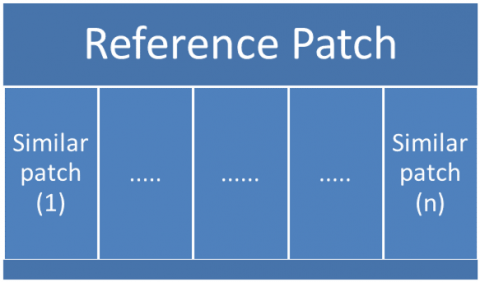
The image denoising method (IDM) in digital pictures has various from virtually unseen. Image denoising measures are aiming to return a novel feature that has less noise, i.e., closer to the novel noise-free feature. IDMs can recognize by two different main approaches: pixel-based picture filtering and patch-based filtering. The first method is a contiguity functional (juxtaposition) exploited operating one pixel and depending on its three dimensional adjacent pixels positioned inside a kernel. While, the second category uses blocks of similar patches, which are then functioned definitely in order to transport an approximation of the main pixel values based on comparable bits located within an observe window. This technique works the termination and the similarity among the frequent segments of the work image (see Figures 1 and 2).
Figure 1. The first category in IDM is a contiguity operation
Figure 2. The second category in IDM uses blocks of similar patches
Mathematically, the issue of image denoising is designed as follows:
$I_{\text {noisy }}=I_{\text {original }}+\alpha$
where, $I_{\text {noisy }}$ is the recognized noisy image, $I_{\text {original }}$ is the original image, and α indicates the additive white Gaussian noise (AWGN) with standard deviation. AWGN is computed in applied presentations by numerous approaches, such as median absolute deviation [35], block-based approximation [36], and standard module analysis [37]. The determination of noise decrease is to reduce the noise in the original pictures while diminishing the loss of imaginative features and refining the signal-to-noise ratio (SNR). The main tests for pictures denoising are as surveys [38]: Smooth areas must be plane, edges must be threatened devoid of blurring, textures must be conserved, and new objects must not be prevented.
3.1 Algorithm
Our algorithm is based on Eqs. (5)-(6). Eq. (5) presents the 1 -D parametric conclusion owning the parameter $\wp$. While Eq. (6) indicated the 2D-parametric conclusion with the parameters $\wp$ and $q$. We shall apply both of these equations to enhance the noisy image. By applying Eqs. (5)-(6), we have the suggested enhanced image:
$I_{\text {noisy }}=I_{\text {original }} * W_{3 \times 3}\left[\Delta_{\wp}\right]$ (7)
and
$I_{\text {noisy }}=I_{\text {original }} * W_{3 \times 3}\left[\Delta_{\wp}(q)\right]$ (8)
respectively, where $*$ indicates the convolution product and $W_{3 \times 3}$ is the window mask of dimension $3 \times 3$.
In this study, different masks are organized as follows:
$\begin{aligned} & W_{0^{\circ}}=\left[\begin{array}{lll}0 & 0 & 0 \\ \Delta_{\wp}(2,1) & \Delta_{\wp}(2,2) & \Delta_{\wp}(2,3) \\ 0 & 0 & 0\end{array}\right] \\ & W_{45^{\circ}}=\left[\begin{array}{lll}0 & 0 & \Delta_{\wp}(1,3) \\ 0 & \Delta_{\wp}(2,2) & 0 \\ \Delta_{\wp}(3,1) & 0 & 0\end{array}\right]\end{aligned}$ (9)
$\begin{gathered}W_{90^{\circ}}=\left[\begin{array}{lll}0 & \Delta_{\wp}(1,2) & 0 \\ 0 & \Delta_{\wp}(2,2) & 0 \\ 0 & \Delta_{\wp}(3,2) & 0\end{array}\right] \\ W_{135^{\circ}}=\left[\begin{array}{lll}\Delta_{\wp}(1,1) & 0 & 0 \\ 0 & \Delta_{\wp}(2,2) & 0 \\ 0 & 0 & \Delta_{\wp}(3,3)\end{array}\right]\end{gathered}$ (10)
Similarly, for $\Delta_{\wp}(q)$ we have the following structures:
$\Psi_{0^{\circ}}=\left[\begin{array}{lll}0 & 0 & 0 \\ \Delta_{\wp}(q)(2,1) & \Delta_{\wp}(q)(2,2) & \Delta_{\wp}(q)(2,3) \\ 0 & 0 & 0\end{array}\right]$ (11)
$\Psi_{45^{\circ}}=\left[\begin{array}{lll}0 & 0 & \Delta_{\wp}(q)(1,3) \\ 0 & \Delta_{\wp}(q)(2,2) & 0 \\ \Delta_{\wp}(q)(3,1) & 0 & 0\end{array}\right]$ (12)
$\Psi_{90^{\circ}}=\left[\begin{array}{ccc}0 & \Delta_{\wp}(q)(1,2) & 0 \\ 0 & \Delta_{\wp}(q)(2,2) & 0 \\ 0 & \Delta_{\wp}(q)(3,2) & 0\end{array}\right]$ (13)
$\Psi_{135^{\circ}}=\left[\begin{array}{lll}\Delta_{\wp}(q)(1,1) & 0 & 0 \\ 0 & \Delta_{\wp}(q)(2,2) & 0 \\ 0 & 0 & \Delta_{\wp}(q)(3,3)\end{array}\right]$ (14)
Our algorithm is given in Figure 3.
Figure 3. The algorithm
In this place, we remark that PNSR (peak signal-to-noise ratio) is a trade span for the ratio between the extreme probable power of a signal (image) and the power of demeaning noise that marks the reliability of its illustration. Because several images have a very varied dynamic variety, PSNR is normally formulated as a logarithmic quantity utilizing the decibel measure. It is formulated by the structure.
$\begin{aligned} P S N R & =10 \cdot \log _{10}\left(\frac{\max (I)^2}{\Sigma}\right) \\ & =20 \cdot \log _{10}\left(\frac{\max (I)}{\sqrt{\Sigma}}\right) \\ & =20 \cdot \log _{10}(\max (I))-10 \cdot \log _{10}(\Sigma)\end{aligned}$
where, max is the maximum value of the pixel and Σ is the mean error:
$\Sigma=\frac{1}{m n} \sum_{i=0}^{m-1} \sum_{j=0}^{n-1}[I(i, j)-\mathrm{⊤}(i, j)]^2$
where, $\mathrm{⊤}$ is the noise image.
Moreover, the root-mean-square error (RMSE) is a regularly utilized ration of the differences between standards expected by a design; or it is an estimator and the principles detected. The RMSD characterizes the square root of the second model moment of the differences between projected tenets and experimental ethics or the quadratic mean of these modifications. It recognized by the following structure:
$\Re=\sqrt{\frac{\sum_{j=1}^n\left(\hat{I}_j-I_j\right)^2}{n}}$
Each pixel in an image possesses a color value that can alter during the process of compression and decompression of the image. Due to the broad spectrum of frequencies in waveforms, PSNR (RMSD) is typically expressed in a logarithmic scale. The relationship is demonstrated through PSNR (RMSD) along with the probability estimate of the pixel, wherein the pixel's number may be indicated by its likelihood. This is particularly true in our method, which depends on the pixel's probability, as outlined in sections 2.5 and 2.6.
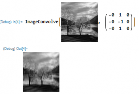
3.2 Convolution matrix
A convolution matrix, often known as a mask, is a tiny matrix used for edge detection, embossing, sharpening, and other effects. Convolution between the kernel and an image is used to achieve this. Alternatively, to put it another way, the kernel is the function that determines how each pixel in the output image is affected by the neighboring in the input image.
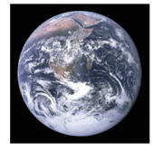
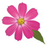
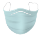
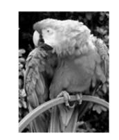
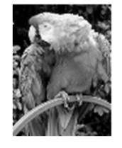
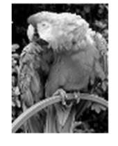
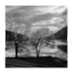
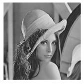
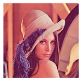
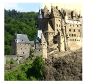
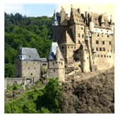
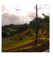
In this section, we illustrate our results by using the suggested information in the above section. Performance calculations were operated by software Mathematica 11.2. The two collections of pictures involved two gray scale images, and two color images. The windows mask of the suggested method is given to be functioned with a 3×3 pixels window (see Figures 4-5).
The calculation presentations of MFD were planned by both PSNR, and RMSD measures. The PSNR values for the transformed values of $\wp$ for (2.5) and $q$ for (2.6), are described in the interval $\wp \in[0,1]$ and $q \in(0,1)$. Table 1 shows the ideal value of PSNR is recognized for the second method (2.6), for all suggested data. The results test by utilizing RMSD have the same conclusion as appeared in Table 2. We compared our method with the reference [6], where the author used one dimensional fractal differential operator. It is clear that our method satisfies a huge enhancement comparing with the results in reference [6]. For future works, one may suggest another description of MFD, using some special functions. Our method can be applied in other field of computer science or studied another type of image processing. Parametric mathematical structures indicate a variety of applications or modification.
(a)
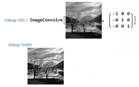
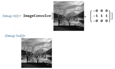
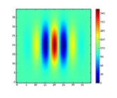
(b)
Figure 4. (a) The convoluted of image with the suggested window $W_{135^{\circ}}$; (b) The convoluted of image with the suggested window $W_{0^{\circ}}$
Table 1. Table to test PNSR
|
Original Image |
MFD (2.5) |
MFD (2.6) |
Ibrahim [6] |
|
35.4221 |
38.9643 |
42.5065 |
31.8799 |
|
21.9361 |
24.1297 |
26.3233 |
19.7425 |
|
26.9325 |
29.6257 |
32.3190 |
24.2392 |
|
28.9911 |
31.8902 |
34.7893 |
26.0920 |
|
37.6823 |
41.4506 |
45.2188 |
33.9141 |
|
25.1448 |
27.6593 |
30.1738 |
22.6304 |
|
24.4467 |
26.8914 |
29.3360 |
22.0020 |
|
26.1336 |
28.7469 |
31.3603 |
23.5202 |
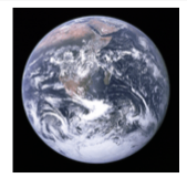
Figure 5. The convoluted of image with the suggested window $W_{90^{\circ}}$
Table 2. Table to test RMSD
|
Original Image |
MFD (2.5) |
MFD (2.6) |
Ibrahim [6] |
|
14.1813 |
15.5995 |
17.0176 |
12.7632 |
|
25.0739 |
27.5813 |
30.0887 |
22.5665 |
|
14.7517 |
16.2269 |
17.7021 |
13.2766 |
|
23.1480 |
25.4629 |
27.7777 |
20.8332 |
|
14.9265 |
16.4192 |
17.9118 |
13.4339 |
|
20.3057 |
22.3363 |
24.3669 |
18.2752 |
Image enhancement refers to the process of improving the visual quality of an image by adjusting its color, contrast, sharpness, and other visual properties. There are several implications of image enhancement, some of which are discussed as follows: Better Visualization: the recent image enhancement technique can help to reveal more details and improve the visual quality of an image, making it easier to interpret and analyze. Moreover, image enhancement technique can be used to improve the quality of surveillance footage, making it easier to identify suspects or suspicious activities. From above by employing the characteristic function to define a new multiscale fractal dimension. As an application, we employed the suggested MFD to define a fractal mask and use it to enhance images. The results showed that our method achieved high test results with the help of PSNR (Table 1) and RMSE (Table 2). Our data set of images is picked form different resources, such as Mathematica, Wikipidia and others. For future effort, one can apply the above method in different types of images such as medical imaging and machine vision systems.
[1] Bioucas-Dias, J.M., Figueiredo, M.A. (2010). Multiplicative noise removal using variable splitting and constrained optimization. IEEE Transactions on Image Processing, 19(7): 1720-1730. https://doi.org/10.1109/TIP.2010.2045029
[2] Yao, W., Guo, Z., Sun, J., Wu, B., Gao, H. (2019). Multiplicative noise removal for texture images based on adaptive anisotropic fractional diffusion equations. SIAM Journal on Imaging Sciences, 12(2): 839-873. https://doi.org/10.1137/18M1187192
[3] Shi, J., Osher, S. (2008). A nonlinear inverse scale space method for a convex multiplicative noise model. SIAM Journal on Imaging Sciences, 1(3): 294-321. https://doi.org/10.1137/070689954
[4] Zhou, Z., Guo, Z., Dong, G., Sun, J., Zhang, D., Wu, B. (2014). A doubly degenerate diffusion model based on the gray level indicator for multiplicative noise removal. IEEE Transactions on Image Processing, 24(1): 249-260. https://doi.org/10.1109/TIP.2014.2376185
[5] Zhang, J., Chen, K. (2015). A total fractional-order variation model for image restoration with nonhomogeneous boundary conditions and its numerical solution. SIAM Journal on Imaging Sciences, 8(4): 2487-2518. https://doi.org/10.1137/14097121X
[6] Ibrahim, R.W. (2020). A new image denoising model utilizing the conformable fractional calculus for multiplicative noise. SN Applied Sciences, 2: 1-11. https://doi.org/10.1007/s42452-019-1718-3
[7] Jalab, H.A., Ibrahim, R.W. (2015). Fractional conway polynomials for image denoising with regularized fractional power parameters. Journal of Mathematical Imaging and Vision, 51: 442-450. https://doi.org/10.1007/s10851-014-0534-z
[8] Jalab, H.A., Ibrahim, R.W. (2015). Fractional Alexander polynomials for image denoising. Signal Processing, 107: 340-354. https://doi.org/10.1016/j.sigpro.2014.06.004
[9] Singh, J., Kumar, D., Baleanu, D., Rathore, S. (2019). On the local fractional wave equation in fractal strings. Mathematical Methods in the Applied Sciences, 42(5): 1588-1595. https://doi.org/10.1002/mma.5458
[10] Ibrahim, R.W., Hasan, A.M., Jalab, H.A. (2018). A new deformable model based on fractional Wright energy function for tumor segmentation of volumetric brain MRI scans. Computer methods and programs in biomedicine, 163: 21-28. https://doi.org/10.1016/j.cmpb.2018.05.031
[11] Al-Shamasneh, A.A.R., Jalab, H.A., Palaiahnakote, S., Obaidellah, U.H., Ibrahim, R.W., El-Melegy, M.T. (2018). A new local fractional entropy-based model for kidney MRI image enhancement. Entropy, 20(5): 344. https://doi.org/10.3390/e20050344
[12] Hasan, A.M., Al-Jawad, M.M., Jalab, H.A., Shaiba, H., Ibrahim, R.W., AL-Shamasneh, A.A.R. (2020). Classification of Covid-19 coronavirus, pneumonia and healthy lungs in CT scans using Q-deformed entropy and deep learning features. Entropy, 22(5): 517. https://doi.org/10.3390/e22050517
[13] Nam, S.H., Choi, J.Y. (1998). A method of image enhancement and fractal dimension for detection of microcalcifications in mammogram. In Proceedings of the 20th Annual International Conference of the IEEE Engineering in Medicine and Biology Society, Hong Kong, China, pp. 1009-1012. https://doi.org/10.1109/IEMBS.1998.745620
[14] Cao, T., Wang, W., Tighe, S., Wang, S. (2019). Crack image detection based on fractional differential and fractal dimension. IET Computer Vision, 13(1): 79-85. https://doi.org/10.1049/iet-cvi.2018.5337
[15] So, G.B., So, H.R., Jin, G.G. (2017). Enhancement of the box-counting algorithm for fractal dimension estimation. Pattern Recognition Letters, 98: 53-58. https://doi.org/10.1016/j.patrec.2017.08.022
[16] Lyu, L., Zhang, D., Tian, Y., Zhou, X. (2021). Sound-absorption performance and fractal dimension feature of kapok fibre/polycaprolactone composites. Coatings, 11(8): 1000. https://doi.org/10.3390/coatings11081000
[17] Al-Azawi, R.J., Al-Saidi, N.M., Jalab, H.A., Kahtan, H., Ibrahim, R.W. (2021). Efficient classification of COVID-19 CT scans by using q-transform model for feature extraction. PeerJ Computer Science, 7: e553. https://doi.org/10.7717/peerj-cs.553
[18] Jalab, H.A., Ibrahim, R.W., Hasan, A.M., Karim, F.K., Al-Shamasneh, A.A.R., Baleanu, D. (2021). A new medical image enhancement algorithm based on fractional calculus. CMC-Computers Materials & Continua, 68(2): 1467-1483. https://doi.org/10.32604/cmc.2021.016047
[19] Al-Azawi, R.J., Al-Saidi, N., Jalab, H.A., Ibrahim, R., Baleanu, D. (2021). Image splicing detection based on texture features with fractal entropy. CMC-Computers Materials & Continua, 69(3): 3903-3915. https://doi.org/10.32604/cmc.2021.020368
[20] Petrou, M.M., Petrou, C. (2010). Image Processing: The Fundamentals. John Wiley & Sons.
[21] Lan, Y., Shu, J. (2019). Fractal dimension of random attractors for non-autonomous fractional stochastic Ginzburg–Landau equations with multiplicative noise. Dynamical Systems, 34(2): 274-300. https://doi.org/10.1080/14689367.2018.1523368
[22] Shahrezaei, I.H., Kim, H.C. (2020). Fractal analysis and texture classification of high-frequency multiplicative noise in SAR sea-ice images based on a transform-domain image decomposition method. IEEE Access, 8: 40198-40223. https://doi.org/10.1109/ACCESS.2020.2976815
[23] Sun, T., Wang, X., Lin, D., Bao, R., Jiang, D., Ding, B., Li, D. (2021). Medical image security authentication method based on wavelet reconstruction and fractal dimension. International Journal of Distributed Sensor Networks, 17(4): 15501477211014132. https://doi.org/10.1177/15501477211014132
[24] Mandelbrot, B.B., Mandelbrot, B.B. (1982). The Fractal Geometry of Nature (Vol. 1). New York: WH Freeman.
[25] Kruk, M., Świderski, B., Osowski, S. (2013). Box-counting fractal dimension in application to recognition of hypertension through the retinal image analysis. Dimension, 500: 1-0573.
[26] Lin, T.P., Hui, H.Y., Ling, A., Chan, P.P., Shen, R., Wong, M. O., Chan, N.C.Y., Leung, D.Y.L., Xu, D., Lee, M.L., Hsu, W., Wong, T.Y., Tham, C.C., Cheung, C.Y. (2023). Risk of normal tension glaucoma progression from automated baseline retinal-vessel caliber analysis: A prospective cohort study. American Journal of Ophthalmology, 247: 111-120. https://doi.org/10.1016/j.ajo.2022.09.015
[27] Huang, F., Dashtbozorg, B., Zhang, J., Bekkers, E., Abbasi-Sureshjani, S., Berendschot, T.T., ter Haar Romeny, B.M. (2016). Reliability of using retinal vascular fractal dimension as a biomarker in the diabetic retinopathy detection. Journal of Ophthalmology, 2016: 6259047. https://doi.org/10.1155/2016/6259047
[28] Rényi, A. (1959). On the dimension and entropy of probability distributions. Acta Mathematica Academiae Scientiarum Hungarica, 10(1-2): 193-215. https://doi.org/10.1007/BF02063299
[29] Kumari, P., Saxena, P. (2023). Automated diabetic retinopathy grading based on the modified capsule network architecture. IETE Journal of Research, 1-12. https://doi.org/10.1080/03772063.2023.2185304
[30] Ţălu, Ş. (2013). Multifractal geometry in analysis and processing of digital retinal photographs for early diagnosis of human diabetic macular edema. Current Eye Research, 38(7): 781-792. https://doi.org/10.3109/02713683.2013.779722
[31] Ott, E. (1993). Chaos in Dynamical Systems. Cambridge University Press: Cambridge, UK; New York, NY, USA.
[32] Yu, S., Lakshminarayanan, V. (2021). Fractal dimension and retinal pathology: A meta-analysis. Applied Sciences, 11(5): 2376. https://doi.org/10.3390/app11052376
[33] Alberti, T., Donner, R.V., Vannitsem, S. (2021). Multiscale fractal dimension analysis of a reduced order model of coupled ocean-Amosphere dynamics. Earth System Dynamics, 12(3): 837-855. https://doi.org/10.5194/esd-12-837-2021
[34] Jones, M.C., Lotwick, H.W. (1983). On the errors involved in computing the empirical characteristic function. Journal of Statistical Computation and Simulation, 17(2): 133-149. https://doi.org/10.1080/00949658308810650
[35] Donoho, D.L., Johnstone, I.M. (1994). Ideal spatial adaptation by wavelet shrinkage. Biometrika, 81(3): 425-455. https://doi.org/10.1093/biomet/81.3.425
[36] Shin, D.H., Park, R.H., Yang, S., Jung, J.H. (2005). Block-based noise estimation using adaptive Gaussian filtering. IEEE Transactions on Consumer Electronics, 51(1): 218-226. https://doi.org/10.1109/TCE.2005.1405723
[37] Liu, W., Lin, W. (2012). Additive white Gaussian noise level estimation in SVD domain for images. IEEE Transactions on Image Processing, 22(3): 872-883. https://doi.org/10.1109/TIP.2012.2219544
[38] Fan, L., Zhang, F., Fan, H., Zhang, C. (2019). Brief review of image denoising techniques. Visual Computing for Industry, Biomedicine, and Art, 2: 1-12. https://doi.org/10.1186/s42492-019-0016-7