Murtadha A. Kadhim*![]() | AllahBakhsh Yazdani Cherati
| AllahBakhsh Yazdani Cherati![]() | Mohammed S. Mechee
| Mohammed S. Mechee![]()
© 2024 The authors. This article is published by IIETA and is licensed under the CC BY 4.0 license (http://creativecommons.org/licenses/by/4.0/).
OPEN ACCESS
Different types of DEs have a wide range of applications in both engineering and science. Typically, when modelling a physical quantity's variation, Recently, it has been found that models based on the theory of fractional-order derivatives and integrals provide an exceptionally good description of a wide range of scientific phenomena. The FDE is a differential equation that contains some derivatives of non-integer powers order. FDEs have become increasingly significant in the theoretical and applied parts of a wide variety of scientific and technical disciplines in recent years. The high-order ODE can be reduced to systems of first order ODEs, which can then be solved. Directly attacking the issue with numerical methods, however, is much more efficient in terms of accuracy, number of function evaluations, and processing time. In this article, the RKM method for solving ordinary differential equations has been introduced. This numerical approach has been generalized to be suitable for solving a class of fractional differential equations (FDEs). However, the developed RKM approach with three- and four-stages for solving sixth-order FODEs is developed. Moreover, this technique was used to solve various test problems, these examples to which the developed method was applied were for various functions with different values of ⍺ and then, the solutions of the developed numerical method were compared with the exact solution, the numerical results proved the efficiency and accuracy of the modified technique.
Runge Kutta (RK), Runge Kutta Direct (RKD), Runge Kutta Mechee (RKM), fractional, ordinary, sixth-order, differential equations (DEs), ordinary differential equations (ODEs), partial differential equations (PDEs), fractional differential equations (FDEs)
The fractional differential equation (FDE) is a differential equation that contains some derivatives of non-integer powers order. FDEs have become increasingly significant in the theoretical and applied parts of a wide variety of scientific and technical disciplines in recent years [1-3].
The higher-order ODE can be reduced to a system of first-order ODEs, which enables for direct numerical solution to the problem. However, the direct method is more efficient in terms of accuracy, number of functions calls, and processing time. So, in recent years the authors have been applied numerical methods to solve several problems of type FDEs for different orders, for examples, Sohaib et al. created Legendre wavelet estimate for sixth-order boundary value problems [4]. Also, Syam and Al-Refai produced a numerical technique dependent on the Chebyshev collocation approach. Atangana-Baleanu fractional derivatives are used to solve linear and nonlinear FDEs [5], Khader et al. [6] used the Chebyshev collocation technique in order to solve the FDEs that arise from the optimization issue, Khalouta and Kadem used the inverse fractional Shehu transform approach for solving linear homogeneous and non-homogeneous FDEs [7]. Cardone et al. [8] developed multivalve collocation techniques, which can be used with both ordinary or FDEs. In 2019, Patrício et al. [9] introduced a novel technique for dealing with initial and boundary value problems in conventional FDEs. However, Hinze et al. proposed a new numerical method for fractional-order ODEs. The method describes the Caputo fractional differential operator in endless states [10], Saqib et al. [11] used Caputo Fabrizio fractional derivative and Laplace transform to solve heat transfer fractional differential equations in a mixed nanofluid. Also, Kumar and Daftardar-Gejji [12] proposed six predictor-corrector systems fixing non-linear FDEs, moreover, Daraghmeh et al. [13] suggested and applied the homotopy perturbation and the matrix approach approaches to get a solution approximation to the linear FDEs. Furthermore, Ahmed [14] used the 4th order Runge-Kutta method then, adapted Runge-Kutta Mersian methods for the purpose of solving initial value problems in Brnoulli's equation involving fractional derivatives, Turkyilmazoglu [15] invented the Adomian decomposition method (ADM) is a classic technique for solving FDEs. In addition to, Nieto [16] constructed an implicit solution to FDEs, plotted the Caputo FDEs and their results are contrasted to those obtained using the traditional logistic equation. In the same way, Mechee and Aidi [17] developed a direct numerical method, for solving FDEs of third order and then, different stages of RKD methods are generated for solving third-order FDEs. As well as, Mechee and Aidi [18] focused on developing first-, second-, and third-stage direct numerical techniques for solving fifth-order partial differential equations and the effectiveness of the new approaches in comparison to the analytical method has been demonstrated via the analysis of numerical examples. In this study, sixth-order FODEs may be introduced and solved using modified RKM methods. Several examples of numerical implementations of the FDEs are used to test the developed approach.
This section introduced some basic concepts for this study.
2.1 Kinds of quasi-linear FODEs of sixth-order
In this subsection some kinds of quasi-linear sixth-order FODEs have been introduced.
2.1.1 Kind of quasi-linear FODEs of sixth-order
The general kinds of quasi-linear FODEs of sixth-order enable written as for solving:
$\begin{gathered}D^{6 \alpha} \mathrm{ỿ}(t)=\mathrm{Ƒ}\left(t, \mathrm{ỿ}(t), \mathrm{ỿ}^{\prime}(t), \mathrm{ỿ}^{\prime \prime}(t), \mathrm{ỿ}^{(3)}(t), \mathrm{ỿ}^{(4)}(t), \mathrm{ỿ}^{(5)}(t)\right), \\ 0<\alpha \leq 1, t \geq t_0,\end{gathered}$
with the initial conditions:
$D^{\mathrm{i} \alpha} \mathrm{ỿ}(0)=\beta_{\mathrm{i}} . \quad \mathrm{i}=0,1,2,3,4,5$. (*)
Kind-One of Quasi-Linear FODEs of Sixth-Order. Consider the kind-one of quasi-linear FODEs sixth-order as follows:
$\begin{gathered}D^{6 \alpha} \mathrm{ỿ}(t)=\mathrm{Ƒ}\left(t, \mathrm{ỿ}(t), \mathrm{ỿ}^{\prime}(t), \mathrm{ỿ}^{\prime \prime}(t), \mathrm{ỿ}^{(3)}(t), \mathrm{ỿ}^{(4)}(t)\right), \\ 0<\alpha \leq 1, t \geq t_0,\end{gathered}$
when the initial conditions in Equation (*).
Kind-Two of Quasi-Linear FODEs of Sixth-Order. Consider the kind-two of quasi-linear FODEs of sixth -order as follows:
$\begin{aligned} D^{6 \alpha} \mathrm{ỿ}(t)= & \mathrm{Ƒ}\left(t, \mathrm{ỿ}(t), \mathrm{ỿ}^{\prime}(t), \mathrm{ỿ}^{\prime \prime}(t), \mathrm{ỿ}^{(3)}(t)\right), \\ & 0<\alpha \leq 1, t \geq t_0,\end{aligned}$
when the initial conditions in Equation (*).
Kind-Three of Quasi-Linear FODEs of Sixth-Order. Consider the kind-three of quasi-linear FODEs of sixth -order as follows:
$\begin{gathered}D^{6 \alpha} \mathrm{ỿ}(t)=\mathrm{Ƒ}\left(t, \mathrm{ỿ}(t), \mathrm{ỿ}^{\prime}(t), \mathrm{ỿ}^{\prime \prime}(t)\right), \\ 0<\alpha \leq 1, t \geq t_0,\end{gathered}$
when the initial conditions in Equation (*).
Kind-Four of Quasi-Linear FODEs of Sixth-Order. Consider the class-four of quasi-linear FODEs of sixth -order as follows:
$\begin{gathered}D^{6 \alpha} \mathrm{ỿ}(t)=\mathrm{Ƒ}\left(t, \mathrm{ỿ}(t), \mathrm{ỿ}^{\prime}(t)\right), \\ 0<\alpha \leq 1, t \geq t_0,\end{gathered}$
when the initial conditions in Equation (*).
Kind-Five of Quasi-Linear FODEs of Sixth-Order. Consider the kind-five of quasi-linear FODEs of sixth -order as follows:
$\begin{aligned} D^{6 \alpha} \mathrm{ỿ}(t)= & \mathrm{Ƒ}(t, \mathrm{ỿ}(t)), t>0,0<\alpha \leq 1, \\ & 0<\alpha \leq 1, t \geq t_0,\end{aligned}$ (1)
when the initial conditions:
$D^{\mathrm{i} \alpha} \mathrm{y}(0)=\beta_{\mathrm{i}} \cdot \mathrm{i}=0,1,2,3,4,5.$ (2)
2.2 RKM method for solving 6th – order ODEs
To solve the class of 6th - order ODEs in Eq. (1) with the initial conditions in Eq. (2), the RKM technique with a s-stage can be written as [18]:
$\begin{gathered}u_{n+1}=u_n+h u_n^{\prime}+\frac{h^2}{2} u_n^{\prime \prime}+\frac{h^3}{6} u_n^{(3)}+\frac{h^4}{24} u_n^{(4)}+\frac{h^5}{120} u_n^{(5)}+h^6 \sum_{i=1}^s \mathrm{~ᶀ}_i^{(0)} \kappa_i,\end{gathered}$ (3)
$\begin{aligned} u_{n+1}^{\prime}= & u_n^{\prime}+h u_n^{\prime \prime}+\frac{h^2}{2} u_n^{(3)}+\frac{h^3}{6} u_n^{(4)}+\frac{h^4}{24} u_n^{(5)}+h^5 \sum_{i=1}^s \mathrm{~ᶀ}_i^{(1)} \kappa_i,\end{aligned}$ (4)
$\begin{gathered}u_{n+1}^{\prime \prime}=u_n^{\prime \prime}+h u_n^{(3)}+\frac{h^2}{2} u_n^{(4)}+\frac{h^3}{6} u_n^{(5)}+h^4 \sum_{i=1}^s \mathrm{~ᶀ}_i^{(2)} \kappa_i,\end{gathered}$ (5)
$u_{n+1}^{(3)}=u_n^{(3)}+h u_n^{(4)}+\frac{h^2}{2} u_n^{(5)}+h^3 \sum_{i=1}^s \mathrm{~ᶀ}_i^{(3)} \kappa_i$ (6)
$u_{n+1}^{(4)}=u_n^{(4)}+h u_n^{(5)}+h^2 \sum_{i=1}^s \mathrm{~ᶀ}_i^{(4)} \kappa_i$ (7)
and
$u_{n+1}^{(5)}=u_n^{(5)}+h \sum_{i=1}^s \mathrm{~ᶀ}_i^{(5)} \kappa_i$. (8)
where,
$\kappa_1=\mathrm{Ƒ}\left(t_n, u_n\right)$, (9)
and
$\begin{aligned} \kappa_i= & \mathrm{Ƒ}\left(t_\eta+c_i h, u_n+h c_i u_n^{\prime}+\frac{h^2}{2} c_i^2 u_n^{\prime \prime}+\frac{h^3}{6} c_i^3 u_n^{(3)}\right. \left.+\frac{h^4}{24} c_i^4 u_n^{(4)}+\frac{h^5}{120} c_i^5 u_n^{(5)}+h^6 \sum_{j=1}^{i-1} a_{i j} \kappa_j\right) .\end{aligned}$ (10)
The parameters of RKM integrator are $a_{i j}, c_i, \mathrm{~Ƒ}_i^{(i i)}$ for $i, j=1$, $2, \ldots, \mathrm{s}, i i=0,1, \ldots, 5$ and $h$ is the size of subintervals RKM method.
In this section, two numerical-methods for solving a quasi- linear FODEs of fifth-order which belong to a class of quasi linear in Eq. (1) with the ICs in Eq. (2) have been constructed in addition to modify another two methods.
3.1 Construction a generalized-Euler method
Taylor expansion of the function u(t+h) can be written as follows:
$\begin{gathered}u(t+h)=u(t)+\frac{h^\alpha}{\Gamma(\alpha+1)} D^\alpha u(t)+ \\ \frac{h^{2 \alpha}}{\Gamma(2 \alpha+1)} D^{2 \alpha} u(t)+\frac{h^{3 \alpha}}{\Gamma(3 \alpha+1)} D^{3 \alpha} u(t)+ \\ \frac{h^{4 \alpha}}{\Gamma(4 \alpha+1)} D^{4 \alpha} u(t)+\frac{h^{5 \alpha}}{\Gamma(5 \alpha+1)} D^{5 \alpha} u(t)+ \\ \frac{h^{6 \alpha}}{\Gamma(6 \alpha+1)} D^{6 \alpha} u(t)+\frac{h^{7 \alpha}}{\Gamma(7 \alpha+1)} D^{7 \alpha} u(t)+\cdots\end{gathered}$. (11)
The higher terms involving $D^{6 \alpha} u(t)$ in Eq. (11) for the very small step-size $h$ have been neglected. Substitute the value of $D^{6 \alpha} u(t)$ from Eq. (11) to obtain the following formula:
$\begin{gathered}u_{n+1 \approx} u_n(t)+\frac{h^\alpha}{\Gamma(\alpha+1)} u_n^\alpha(t)+\frac{h^{2 \alpha}}{\Gamma(2 \alpha+1)} u_n^{2 \alpha}(t)+ \\ \frac{h^{3 \alpha}}{\Gamma(3 \alpha+1)} u_n^{3 \alpha}(t)+\frac{h^{4 \alpha}}{\Gamma(4 \alpha+1)} u_n^{4 \alpha}(t) \\ +\frac{h^{5 \alpha}}{\Gamma(5 \alpha+1)} u_n^{5 \alpha}(t)+\frac{h^{6 \alpha}}{\Gamma(6 \alpha+1)} \Phi\left(t_n, u_n(t)\right) .\end{gathered}$ (12)
By taking a derivative to two sides of Eq. (12) five times to obtain the following equations:
$\begin{gathered}u_{n+1}^\alpha=u_n^\alpha(t)+\frac{h^\alpha}{\Gamma(\alpha+1)} u_n^{2 \alpha}+\frac{h^{2 \alpha}}{\Gamma(2 \alpha+1)} u_n^{3 \alpha}(t)+ \\ \frac{h^{3 \alpha}}{\Gamma(3 \alpha+1)} u_n^{4 \alpha}(t)+\frac{h^{4 \alpha}}{\Gamma(4 \alpha+1)} u_n^{5 \alpha}(t)+ \\ \frac{h^{5 \alpha}}{\Gamma(5 \alpha+1)} \Phi\left(t_n, u_n(t)\right),\end{gathered}$ (13)
$\begin{gathered}u_{n+1}^{2 \alpha}=u_n^{2 \alpha}(t)+\frac{h^\alpha}{\Gamma(\alpha+1)} u_n^{3 \alpha}+\frac{h^{2 \alpha}}{\Gamma(2 \alpha+1)} u_n^{4 \alpha}+ \\ \frac{h^{3 \alpha}}{\Gamma(3 \alpha+1)} u_n^{5 \alpha}(t)+\frac{h^{3 \alpha}}{\Gamma(3 \alpha+1)} \Phi\left(t_n, u_n(t)\right),\end{gathered}$ (14)
$\begin{gathered}u_{n+1}^{3 \alpha}=u_n^{3 \alpha}+\frac{h^\alpha}{\Gamma(\alpha+1)} u_n^{4 \alpha}+\frac{h^{2 \alpha}}{\Gamma(2 \alpha+1)} u_n^{5 \alpha}(t)+ \\ \frac{h^{3 \alpha}}{\Gamma(3 \alpha+1)} \Phi\left(t_n, u_n(t)\right),\end{gathered}$ (15)
$u_{n+1}^{4 \alpha}=u_n^{4 \alpha}+\frac{h^\alpha}{\Gamma(\alpha+1)} u_n^{5 \alpha}+\frac{h^{2 \alpha}}{\Gamma(2 \alpha+1)} \Phi\left(t_n, u_n(t)\right)$, (16)
and
$u_{n+1}^{5 \alpha}=u_n^{5 \alpha}+\frac{h^\alpha}{\Gamma(\alpha+1)} \Phi\left(t_n, u_n(t)\right)$. (17)
The formulas in Eqs. (12)-(17) used to generate a convergent- sequence of solutions for solving the FDEs in Eq. (1) with the ICs in Eq. (2).
3.2 Derivation of developed RKM-method of two-stages
To derive RKM-method, we used the chain rule to obtain the following formula:
$\begin{gathered}\mathrm{D}^{7 \alpha} u(\mathrm{t})=\mathrm{D}^\alpha\left(\mathrm{D}^{6 \alpha} u(\mathrm{t})\right)=\mathrm{D}^\alpha(\Phi(\mathrm{t}, u(\mathrm{t})))= \\ \mathrm{D}^\alpha\left(\Phi(\mathrm{t}, u(\mathrm{t}))+\Phi(\mathrm{t}, u(\mathrm{t})) \mathrm{D}_u^\alpha \Phi(\mathrm{t}, u(\mathrm{t})) .\right.\end{gathered}$ (18)
The higher terms which involve $\mathrm{D}^{7 \alpha} u(\mathrm{t})$ in Eq. (18) for the very small step-size have been neglected. Substitute the value of $\mathrm{D}^{7 \alpha} u(\mathrm{t})$ from Eq. (12) to obtain the following formula:
$\begin{gathered}u_{n+1}=u_n(\mathrm{t})+\frac{\mathrm{h}^\alpha}{\Gamma(\alpha+1)} u_n^\alpha(\mathrm{t})+\frac{\mathrm{h}^{2 \alpha}}{\Gamma(2 \alpha+1)} u_n^{2 \alpha}(\mathrm{t})+ \\ \frac{\mathrm{h}^{3 \alpha}}{\Gamma(3 \alpha+1)} u_n^{3 \alpha}(\mathrm{t})+\frac{\mathrm{h}^{4 \alpha}}{\Gamma(4 \alpha+1)} u_n^{4 \alpha}(\mathrm{t})+\frac{\mathrm{h}^{5 \alpha}}{\Gamma(5 \alpha+1)} u_n^{5 \alpha}(\mathrm{t})+ \\ \frac{\mathrm{h}^{6 \alpha}}{\Gamma(6 \alpha+1)} \Phi\left(\mathrm{t}_n, u_n\left(t_n\right)\right)+\frac{\mathrm{h}^{7 \alpha}}{\Gamma(7 \alpha+1)}\left(\mathrm{D}^\alpha\left(\Phi\left(t_n, u\left(t_n\right)\right)+\right.\right. \\ \Phi\left(t_n, u\left(t_n\right)\right) \mathrm{D}_u^\alpha \Phi\left(t_n, u\left(t_n\right)\right)= \\ u_n(\mathrm{t})+\frac{\mathrm{h}^\alpha}{\Gamma(\alpha+1)} u_n^\alpha(\mathrm{t})+\frac{\mathrm{h}^{2 \alpha}}{\Gamma(2 \alpha+1)} u_n^{2 \alpha}(\mathrm{t})+ \\ \frac{\mathrm{h}^{3 \alpha}}{\Gamma(3 \alpha+1)} u_n^{3 \alpha}(\mathrm{t})+\frac{\mathrm{h}^{4 \alpha}}{\Gamma(4 \alpha+1)} u_n^{4 \alpha}(\mathrm{t})+\frac{\mathrm{h}^{5 \alpha}}{\Gamma(5 \alpha+1)} u_n^{5 \alpha}(\mathrm{t})+ \\ \frac{\mathrm{h}^{6 \alpha}}{2 \Gamma(6 \alpha+1)} \Phi\left(\mathrm{t}_n, u_n\left(t_n\right)\right)+\frac{\mathrm{h}^{6 \alpha}}{2 \Gamma(6 \alpha+1)} \Phi(\mathrm{t}+ \\ \left.\frac{2 \mathrm{~h}^{6 \alpha} \Gamma(6 \alpha+1)}{\Gamma(7 \alpha+1)}, u(\mathrm{t})+\frac{2 \mathrm{~h}^{6 \alpha} \Gamma(6 \alpha+1)}{\Gamma(7 \alpha+1)} \Phi\left(\mathrm{t}_n, u_n\left(\mathrm{t}_n\right)\right)\right) .\end{gathered}$ (19)
By making the derivations to FDE in Eq. (19) once and twice to obtain the following:
$\begin{gathered}u_{n+1}^\alpha=u_{\mathrm{n}}^\alpha(\mathrm{t})+\frac{\mathrm{h}^\alpha}{\Gamma(\alpha+1)} u_n^{2 \alpha}(\mathrm{t})+\frac{\mathrm{h}^{2 \alpha}}{\Gamma(2 \alpha+1)} u_n^{3 \alpha}(\mathrm{t})+ \\ \frac{\mathrm{h}^{3 \alpha}}{\Gamma(3 \alpha+1)} u_n^{4 \alpha}(\mathrm{t})+\frac{\mathrm{h}^{4 \alpha}}{\Gamma(4 \alpha+1)} u_n^{5 \alpha}(\mathrm{t})+ \\ \frac{\mathrm{h}^{5 \alpha}}{\Gamma(5 \alpha+1)} \Phi\left(\mathrm{t}_n, u_n(\mathrm{t})\right) .\end{gathered}$ (20)
However, using the formulas in Eqs. (15)-(20) give a convergent sequence for solving Eq. (1) with the initial conditions in Eq. (2).
3.3 Developed RKM method for solving 6th–order FDEs
To develop the formulas in Eqs. (3)-(9) for solving 6th order ODEs to be appropriate for solving 6th order FDEs, we presume the following formula to approximate the numerical solutions of Eq. (1) with initial conditions in Eq. (2)
$\begin{gathered}u_{n+1}\left(t_n\right)=u_n\left(t_n\right)+\frac{h^\alpha}{\Gamma(\alpha+1)} D^\alpha u_n\left(t_n\right)+ \\ \frac{h^{2 \alpha}}{\Gamma(2 \alpha+1)} D^{2 \alpha} u_n\left(t_n\right)+\frac{h^{3 \alpha}}{\Gamma(3 \alpha+1)} D^{3 \alpha} u_n\left(t_n\right)+ \\ \frac{h^{4 \alpha}}{\Gamma(4 \alpha+1)} D^{4 \alpha} u_n\left(t_n\right)+\frac{h^{5 \alpha}}{\Gamma(5 \alpha+1)} D^{5 \alpha} u_n\left(t_n\right)+ \\ h^{6 \alpha} \sum_{i=1}^s \mathrm{~ᶀ}_i^{(0)} \kappa_1,\end{gathered}$ (21)
$\begin{gathered}u_{n+1}^\alpha\left(t_n\right)=D^\alpha u_n\left(t_n\right)+\frac{h^\alpha}{\Gamma(\alpha+1)} D^{2 \alpha} u_n\left(t_n\right)+ \\ \frac{h^{2 \alpha}}{\Gamma(2 \alpha+1)} D^{3 \alpha} u_n\left(t_n\right)+\frac{h^{3 \alpha}}{\Gamma(3 \alpha+1)} D^{4 \alpha} u_n\left(t_n\right)+ \\ \frac{h^{4 \alpha}}{\Gamma(4 \alpha+1)} D^{5 \alpha} u_n\left(t_n\right)+h^{5 \alpha} \sum_{i=1}^s ᶀ_i^{(1)} \kappa_i,\end{gathered}$ (22)
$\begin{gathered}u_{n+1}^{2 \alpha}\left(t_n\right)=D^{2 \alpha} u_n\left(t_n\right)+\frac{h^\alpha}{\Gamma(\alpha+1)} D^{3 \alpha} u_n\left(t_n\right) \\ +\frac{h^{2 \alpha}}{\Gamma(2 \alpha+1)} D^{4 \alpha} u_n\left(t_n\right)+\frac{h^{3 \alpha}}{\Gamma(3 \alpha+1)} D^{5 \alpha} u_n\left(t_n\right) \\ +h^{4 \alpha} \sum_{i=1}^s \mathrm{~ᶀ}_i^{(2)} \kappa_i,\end{gathered}$ (23)
$\begin{gathered}u_{n+1}^{3 \alpha}\left(t_n\right)=D^{3 \alpha} u_n\left(t_n\right)+\frac{h^\alpha}{\Gamma(\alpha+1)} D^{4 \alpha} u_n\left(t_n\right) \\ +\frac{h^{2 \alpha}}{\Gamma(2 \alpha+1)} D^{5 \alpha} u_n\left(t_n\right)+h^{3 \alpha} \sum_{i=1}^s \mathrm{~ᶀ}_i^{(3)} \kappa_i\end{gathered}$ (24)
$\begin{gathered}u_{n+1}^{4 \alpha}\left(t_n\right)=D^{4 \alpha} u_n\left(t_n\right)+\frac{h^\alpha}{\Gamma(\alpha+1)} D^{5 \alpha} u_n\left(t_n\right) \\ +h^{2 \alpha} \sum_{i=1}^s \mathrm{~ᶀ}_i^{(4)} \kappa_i,\end{gathered}$ (25)
and
$u_{n+1}^{5 \alpha}\left(t_n\right)=D^{5 \alpha} u_n\left(t_n\right)+h^\alpha \sum_{i=1}^s ᶀ_i^{(5)} \kappa_i$ (26)
where,
$\kappa_1=\mathrm{Ƒ}\left(t_n, u_n\left(t_n\right)\right)$, (27)
and
\begin{gathered}\mathrm{K}_i=\mathrm{Ƒ}\left(t_n+c_i h, u_n+h c_i u_n^{\prime}+\frac{h^2}{2} c_i^2 u_n^{\prime \prime}+\frac{h^3}{6} c_i^3 u_n^{(3)}+\right.\left.\frac{h^4}{24} c_i^4 u_n^{(4)}+\frac{h^5}{120} c_i^5 u_n^{(5)}+h^6 \sum_{j=1}^{i-1} a_{i j} \mathrm{~K}_j\right). \end{gathered} (28)
The parameters of RKM integrator are $a_{i j}, c_i, \mathrm{~ᶀ}_i^{(i i)}$ for $i, j=$ $1,2, \ldots, s, i i=0,1, \ldots, 5$ are assumed to be real. If $a_{i j}=0$ for $i \leq j$, it is an explicit method and implicit otherwise. In Butcher tables of coefficients, the RKM methods which can be expressed in the Table 1, Table 2 and Table 3.
Table 1. Butcher Tableau RKM method
|
C |
Α |
|
|
$\mathrm{b}^{\mathrm{T}}$ $\mathrm{b}^{\prime \mathrm{T}}$ $\mathrm{b}^{\prime \prime \mathrm{T}}$ $b^{(3) T}$ $b^{(4) T}$ $b^{(5) T}$ |
Table 2. The Butcher Tableau RKM5 method
|
$\frac{1}{2}+\frac{\sqrt{15}}{10}$ |
$0$ |
|
$\frac{1}{2}-\frac{\sqrt{15}}{10}$ |
$\begin{array}{lll}\frac{1}{2} & 0 & 0\end{array}$ |
|
$\frac{1}{2}$ |
$\begin{array}{lll}\frac{1}{2} & -\frac{1}{2} & 0\end{array}$ |
|
$\frac{11}{17280}+\frac{71 \sqrt{15}}{432000} \quad \frac{11}{17280}-\frac{71 \sqrt{15}}{432000} \quad \frac{1}{8640}$ $\frac{31}{8640}+\frac{\sqrt{15}}{1080} \quad \frac{31}{172808640}-\frac{\sqrt{15}}{1080} \quad \frac{1}{864}$ $\frac{7}{432}+\frac{\sqrt{15}}{240} \quad \frac{7}{432}-\frac{\sqrt{15}}{240} \quad \frac{1}{108}$ $\frac{1}{18}+\frac{\sqrt{15}}{72} \quad \frac{1}{18}-\frac{\sqrt{15}}{72} \quad \frac{1}{18}$ $\frac{5}{36}-\frac{\sqrt{15}}{36} \quad \frac{5}{36}-\frac{\sqrt{15}}{36} \quad \frac{2}{9}$ $\frac{5}{18} \quad \frac{5}{18} \quad \frac{4}{9}$ |
Table 3. The Butcher Tableau RKM6 method
|
|
$\frac{1}{2}+\frac{\sqrt{15}}{10} \quad \frac{1}{2}-\frac{\sqrt{15}}{10} \quad-\frac{2956321}{50400}-\frac{745387 \sqrt{15}}{50400} \quad 0$ $\frac{1}{2} \quad-\frac{2981521}{50400}-\frac{372689 \sqrt{5}}{25200}-\frac{372689 \sqrt{15}}{25200} \quad 0$ $\frac{1}{2} \quad \frac{11835427}{161280}+\frac{15144271}{806400}-\frac{10079}{17920}-\frac{33803 \sqrt{15}}{115200} \quad 0$ |
|
$\frac{11}{17280}+\frac{71 \sqrt{15}}{432000} \quad \frac{1}{2}+\frac{\sqrt{15}}{432000} \quad \frac{11}{17280}$ $-\frac{71 \sqrt{15}}{432000} \quad \frac{1}{8640}$ $\frac{31}{8640}+\frac{\sqrt{15}}{1080} \quad \frac{31}{172808640}-\frac{\sqrt{15}}{1080}$ $\frac{1}{864} \quad 0$ $\frac{7}{432}+\frac{\sqrt{15}}{240} \quad \frac{7}{432}-\frac{\sqrt{15}}{240}$ $\frac{1}{108} \quad 0$ $\frac{1}{18}+\frac{\sqrt{15}}{72} \quad \frac{1}{18}-\frac{\sqrt{15}}{72}$ $\frac{2}{9} \quad 0$ |
In this part, we use numerical results of test examples to show the efficacy of the developed approach:
Example 4.1
Consider the 6th - order FODE in the following:
$D^{6 \alpha} \mathrm{ỿ}(t)=a^{6 \alpha} \mathrm{ỿ}(t), \quad 0<\alpha<1$, (29)
with the initial conditions
$\left.\mathrm{ỿ}(t)\right|_{t=0}=1,\left.D^{n \alpha} \mathrm{ỿ}(t)\right|_{t=0}=a^{n \alpha}, n=1,2,3,4,5.$
The exact solution is $\mathrm{ỿ}(\mathrm{t})=e^{a \mathrm{t}}$.
Example 4.2
Consider the 6th - order FODE in the following:
$D^{6 \alpha} ỿ(t)=a^{6 \alpha} \cos (a t+3 \pi \alpha), 0<\alpha<1$, (30)
with the initial conditions:
$\begin{gathered}\left.ỿ(t)\right|_{t=0}=1, \\ \left.D^\alpha y(t)\right|_{t=0}=a^\alpha \cos \left(\frac{\pi \alpha}{2}\right), \\ \left.D^{2 \alpha} ỿ(t)\right|_{t=0}=a^{2 \alpha} \cos (\pi \alpha), \\ \left.D^{3 \alpha} y(t)\right|_{t=0}=a^{3 \alpha} \cos \left(\frac{3 \pi \alpha}{2}\right), \\ \left.D^{4 \alpha} ỿ(t)\right|_{t=0}=a^{4 \alpha} \cos (2 \pi \alpha), \\ \left.D^{5 \alpha} y(t)\right|_{t=0}=a^{5 \alpha} \cos \left(\frac{5 \pi \alpha}{2}\right) .\end{gathered}$
The exact solution is $ỿ(t)=\cos (a t)$.
Example 4.3
Consider the 6th - order FODE in the following:
$D^{6 \alpha} \mathrm{ỿ}(t)=a^{6 \alpha} \sin (a t+3 \pi \alpha), 0<\alpha<1$, (31)
with the initial conditions:
$\begin{gathered}\left.ỿ(t)\right|_{t=0}=0, \\ \left.D^\alpha \mathrm{ỿ}(t)\right|_{t=0}=a^\alpha \sin \left(\frac{\Pi \alpha}{2}\right), \\ \left.D^{2 \alpha} \mathrm{ỿ}(t)\right|_{t=0}=a^{2 \alpha} \sin (\pi \alpha), \\ \left.D^{3 \alpha} \mathrm{ỿ}(t)\right|_{t=0}=a^{3 \alpha} \sin \left(\frac{3 \pi \alpha}{2}\right), \\ \left.D^{4 \alpha} \mathrm{ỿ}(t)\right|_{t=0}=a^{4 \alpha} \sin (2 \pi \alpha), \\ \left.D^{5 \alpha} \mathrm{ỿ}(t)\right|_{t=0}=a^{5 \alpha} \sin \left(\frac{5 \pi \alpha}{2}\right) .\end{gathered}$
The exact solution is $ỿ(t)=\sin (a t)$.
Example 4.4
Consider the 6th - order FODE in the following
$\begin{aligned} & D^{6 \alpha} \mathrm{ỿ}(t)=\mathrm{ỿ}(t)-t^{2-6 \alpha}\left(\frac{1-2 \alpha}{\Gamma(-6 \alpha+1)\left(11 \alpha-36 \alpha^2+36 \alpha^3-1\right)}\right), \\ & \frac{1}{6}<\alpha \& \alpha \neq \frac{1}{2} \& \alpha \neq \frac{1}{3} \\ & \end{aligned}$
with the initial conditions:
$\left.D^{(n \alpha)} \mathrm{ỿ}(t)\right|_{t=0}=0, \mathrm{\eta}=0,1,2,3,4,5$.
The exact solution is $ỿ(t)=t^2$.
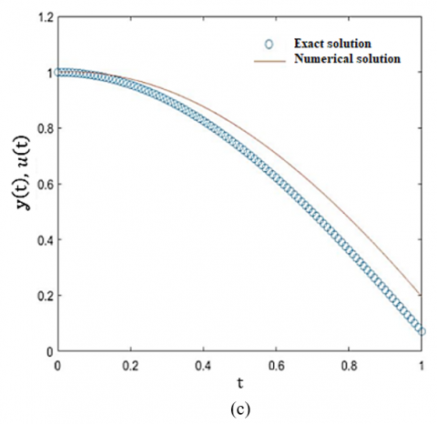
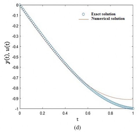
A comparison between the numerical solutions $u(t)$ evaluated by Generalized RKM method versus the exact solutions $\mathrm{ỿ}(\mathrm{t})$ for the above examples is shown in Figure 1.
Figure 1. A comparison on approximated solutions versus analytical solutions for example: (a) $4.1, a=-2.5, \alpha=0.96$; (b) 4.2 , $a=1.2, \alpha=0.93$; (c) $4.2, a=1.2, \alpha=0.97$; (d) $4.3, a=-1.5, \alpha=0.96$ and (e) $4.4, \alpha=0.67$ with $\mathrm{N}=1000$
In this work, we developed the direct RKM numerical methods for solving ODEs of 6th - order, RKM methods have been modified to be consistent for solving FDEs. The effectiveness of the proposed techniques is shown via an assortment of examples of 6th - order FODEs. Compared with the exact solutions, the developed numerical methods demonstrated good agreement (see Figure 1). The novel methods have been effective and they produced excellent results. In this paper, we develop the direct methods with third- and fifth-stages explicit RKM techniques of constant step-sizes for solving 6th - order FODEs. These numerical methods employ less function evaluations and demonstrate good agreement with the analytical solutions. Due to the modified RKM method being a direct method, it significantly reduces the amount of time spent on computations. When compared to the other techniques, this one requires less time and resources to compute. To verify the reliability of the method, the numerical solutions are compared to previously determined exact solutions. The technique's numerical findings confirm their applicability to FODEs.
[1] Hattaf, K., Yousfi, N. (2020). Global stability for fractional diffusion equations in biological systems. Complexity, 2020: 1-6. https://doi.org/10.1155/2020/5476842
[2] Magin, R.L. (2010). Fractional calculus models of complex dynamics in biological tissues. Computers & Mathematics with Applications, 59(5): 1586-1593. https://doi.org/10.1016/j.camwa.2009.08.039
[3] Cheneke, K.R., Rao, K.P., Edessa, G.K. (2021). Application of a new generalized fractional derivative and rank of control measures on cholera transmission dynamics. International Journal of Mathematics and Mathematical Sciences, 2021: 1-9. https://doi.org/10.1155/2021/2104051
[4] Sohaib, M., Haq, S., Mukhtar, S., Khan, I. (2018). Numerical solution of sixth-order boundary-value problems using Legendre wavelet collocation method. Results in Physics, 8: 1204-1208. https://doi.org/10.1016/j.rinp.2018.01.065
[5] Syam, M.I., Al-Refai, M. (2019). Fractional differential equations with Atangana–Baleanu fractional derivative: Analysis and applications. Chaos, Solitons & Fractals: X, 2: 100013. https://doi.org/10.1016/j.csfx.2019.100013
[6] Khader, M.M., Sweilam, N.H., Mahdy, A.M.S. (2013). Numerical study for the fractional differential equations generated by optimization problem using Chebyshev collocation method and FDM. Applied Mathematics & Information Sciences, 7(5): 2011-2018. http://doi.org/10.12785/amis/070541
[7] Khalouta, A., Kadem, A. (2019). A new method to solve fractional differential equations: Inverse fractional Shehu transform method. Applications and Applied Mathematics: An International Journal (AAM), 14(2): 19.
[8] Cardone, A., Conte, D., D’Ambrosio, R., Paternoster, B. (2022). Multivalue collocation methods for ordinary and fractional differential equations. Mathematics, 10(2): 185. https://doi.org/10.3390/math10020185
[9] Patrício, M.S., Ramos, H., Patrício, M. (2019). Solving initial and boundary value problems of fractional ordinary differential equations by using collocation and fractional powers. Journal of Computational and Applied Mathematics, 354: 348-359. https://doi.org/10.1016/j.cam.2018.07.034
[10] Hinze, M., Schmidt, A., Leine, R.I. (2019). Numerical solution of fractional-order ordinary differential equations using the reformulated infinite state representation. Fractional Calculus and Applied Analysis, 22(5): 1321-1350. https://doi.org/10.1515/fca-2019-0070
[11] Saqib, M., Khan, I., Shafie, S. (2019). Application of fractional differential equations to heat transfer in hybrid nanofluid: Modeling and solution via integral transforms. Advances in Difference Equations, 2019(1): 1-18. https://doi.org/10.1186/s13662-019-1988-5
[12] Kumar, M., Daftardar-Gejji, V. (2019). A new family of predictor-corrector methods for solving fractional differential equations. Applied Mathematics and Computation, 363: 124633. https://doi.org/10.1016/j.amc.2019.124633
[13] Daraghmeh, A., Qatanani, N., Saadeh, A. (2020). Numerical solution of fractional differential equations. Applied Mathematics, 11(11): 1100-1115. https://doi.org/10.4236/am.2020.1111074
[14] Ahmed, M.M. (2021). Numerical solutions of Bernoulli differential equations with fractional derivatives by Runge-Kutta techniques. Journal of Humanitarian and Applied Sciences, 11: 272-288.
[15] Turkyilmazoglu, M. (2022). An efficient computational method for differential equations of fractional type. CMES-Computer Modeling in Engineering & Sciences, 133(1): 47-65. http://doi.org/10.32604/cmes.2022.020781
[16] Nieto, J.J. (2022). Solution of a fractional logistic ordinary differential equation. Applied Mathematics Letters, 123: 107568. https://doi.org/10.1016/j.aml.2021.107568
[17] Mechee, M.S., Aidi, S.H. (2022). Generalized Euler and Runge-Kutta methods for solving classes of fractional ordinary differential equations. International Journal of Nonlinear Analysis and Applications, 13(1): 1737-1745. https://doi.org/10.22075/ijnaa.2022.5788
[18] Mechee, M.S., Aidi, S.H. (2023). Constructing RKM-method for solving fractional ordinary differential equations of fifth-order with applications. Ibn AL-Haitham Journal for Pure and Applied Sciences, 36(3): 416-426. https://doi.org/10.30526/36.3.3033