Adedeji Tomide Akindadelo![]() | Folorunsho A. Shodiya
| Folorunsho A. Shodiya![]() | Ayodeji Olalekan Salau*
| Ayodeji Olalekan Salau*![]() | Olawale Joshua Olaluyi
| Olawale Joshua Olaluyi![]() | Jeremiah Oluwatosin Bandele
| Jeremiah Oluwatosin Bandele![]() | Sepiribo Lucky Braide
| Sepiribo Lucky Braide![]()
© 2024 The authors. This article is published by IIETA and is licensed under the CC BY 4.0 license (http://creativecommons.org/licenses/by/4.0/).
OPEN ACCESS
Load flow is an important tool for studying, designing, and analyzing power systems. It allows power system engineers to determine whether the operation and configuration of the power system is safe under varying loading conditions. It is necessary to model and simulate such a system in order to determine the power flow and losses. This research paper focuses on using numerical methods such as Newton Raphson and Gauss Seidel power flow equations for load flow analysis to calculate bus voltage magnitudes, phase angles, real and reactive power of each bus of an IEEE 9-bus test system. Newton Raphson’s computation offers fast, accurate convergence but demands complex implementation, whereas Gauss Siedel is simpler but converges slower with lower accuracy. The analysis was carried out using a MATLAB program. By manipulating variables such as power injections, voltage magnitudes, and phase angles, it solves nonlinear equations iteratively to establish stable operating points which aids in enhancing power system analysis. The line losses for the two methods are compared and the system's total load and generation power are also displayed. The consideration of line losses and assessment of total load generation is crucial for maintaining system efficiency, reliability and preventing voltage instability and equipment damage. The results are also used to generate a directed graph which shows the interconnected nature of the power system, aiding engineers in understanding power flow paths, identifying potential issues, and making informed decisions about system operations. The Newton Raphson method yields the lowest loss, with 4.585MW and 10.789Mvar. In comparison, the Gauss Seidel method achieved 4.809MW and 10.798Mvar.
power flow, bus, load flow analysis, loss minimization, gauss-seidel, Newton-Raphson, voltage magnitude, phase angle, real power, reactive power, convergence
Power flow analysis, also known as load flow analysis, is the foundation of voltage-current system analysis and design. The study of power flow analysis is essential to understanding problems in voltage-current system operation and distribution. It is also a fundamental technique in electrical engineering that enables the planning, operation, and optimization of power systems by determining steady-state conditions, ensuring reliability, efficiency, and the integration of renewable sources, and facilitating informed decision-making for grid stability and resource utilization. The goal of such an analysis is to determine how safely the system can work, i.e., whether there are installation overloads or extremely high or extremely low voltages nodes. It also provides more information about all of the system's components, ensuring that each generator operates at its optimal performing level that consumer’s needs are achieved without overloading the facilities, and that plans for maintenance can be carried out without jeopardizing the system's network. Load flow investigations also provide a mathematical methodology for calculating different bus voltages, phase angles, real power (A) and reactive power flow (B) via various nodes under steady-state conditions [1]. It also aids in determining the impact of a single generating station or transmission path failure on the load system. Moreover, it provides a balanced steady-state operation state of the load system while ignoring a non-steady process system. This means that any load flow problem's mathematical formulation is a nonlinear algebraic equation system without differential equations. As a result, using prepared algorithms and programs for load flow analysis is critical for performing recent load system analysis.
Over the years, different methods have been used for calculating load flow. The use of these methods is primarily driven by the fundamental requirements of power flow calculation, which include its iteration properties, computing accuracy and storage requirements, as well as its convenience and flexibility of implementation [2-5].
The power flow problem is a system of nonlinear algebraic equations that must be solved mathematically. Its answer will almost always require some iteration. As a result, the most crucial condition for a load flow calculation method is reliable convergence. The dimension of load flow equations grows increasingly large as the size of the load system expands. Thus, the power flow analysis is becoming increasingly important for equations with such high dimensions.
In this work, power flow analysis using the Newton Raphson method and Gauss-Seidel on an IEEE standard 9 bus test system is compared. The 9-bus test system is a simplified model of an electrical power network used for analyzing power system techniques. It comprises 9 buses, including a slack bus with known values, load buses with demand, a generator bus with both load and generation, and branches representing connections between buses. Loads and generation are specified at certain buses, and the system is used to study power flow, voltage profiles, and stability under various conditions.
In the realm of power system analysis, methods for solving the power flow equations play a pivotal role in ensuring the efficient and reliable operation of electrical networks. Two widely employed techniques for solving these equations are the Newton-Raphson and Gauss-Seidel methods. This study aims to compare and evaluate the performance of these methods in the context of power flow analysis. By systematically assessing their convergence characteristics, computational efficiency, and accuracy, we seek to gain insights into their respective strengths and limitations. This study compares the Newton-Raphson and Gauss-Seidel methods for power flow analysis on the IEEE 9-bus test system, focusing on convergence, accuracy, and efficiency. The simulation setup involves replicating the system, implementing methods with defined criteria, and running analyses. Through this analysis, we aim to provide valuable guidance for selecting the most suitable method based on specific application scenarios, contributing to the advancement of power system analysis techniques and the optimization of electrical grid operation.
The node that connects more lines, more loads, and more generators is termed BUS. In a load system, every bus is accompanied with the following parameters: $|V|$, voltage phase angle (<), real power (A), and reactive power (B) in which two parameters are known and the other must be determined by solving equation [3]. The buses are categorize based on the parameters specified, as shown in Table 1.
2.1 Load bus (AB)
The real power A and reactive power B of the load bus are specified, while the |V| and phase angle $(<)$ of the voltage are not specified [6, 7]. The bus voltage is determined using power flow analysis. Voltage on the load bus can vary within certain boundaries, say 5%. The reason why the bus voltage is insignificant and therefore not mentioned. This bus is in charge of distributing consumer power.
Table 1. BUS type
|
Type |
Known Parameter |
Unknown Parameter |
|
Load BUS |
A, B (Real and Reactive Power) |
|V|, < |
|
Generator BUS |
|V|, A |
B, < |
|
Swing BUS |
|V|, < |
B, A |
2.2 Voltage controlled or generator bus
Swing or Reference Bus are other names for Slack Bus. This in reality does not come to play but it is believed to account for losses that arises when transmitting power. In the power system, real power is specified for only two buses: the Load Bus and the Generator Bus. Because the real power delivered by Generator Bus differs from the real power consumed by Load Bus, the difference gives the power loss. This loss is then calculated after the load flow problem has been solved. To compensate for the loss, an additional generator bus is considered, with |V|, and phase angle specified, and real and reactive power to be solved. Some additional buses that are considered in performing load flow analysis.
2.3 Isolated (or dummy) bus
An isolated bus is used to represent an unconnected or isolated portion of the power system. It is used when there are areas in the network where there are no direct connections to other buses.
2.4 Slackless (or zero injection) bus
In certain situations, such as load flow analysis with constant power loads, a slackless bus can be used to represent the system's behavior more accurately. This type of bus helps avoid some of the inaccuracies that can arise when using a traditional slack bus. The Bus data table for the IEEE 3-bus system is presented in Table 2.
Table 2. Bus data table for the IEEE 3-bus system
|
Bus Number |
Bus Type |
Voltage Magnitude (pu) |
Voltage Angle (degrees) |
Active Power (MW) |
Reactive Power (MVAR) |
|
1 |
Swing |
1.0 |
0 |
Adjustable |
Adjustable |
|
2 |
PV |
1.05 |
Adjustable |
1.0 |
Adjustable |
|
3 |
PQ |
Adjustable |
Adjustable |
0.8 |
0.4 |
The IEEE 3-bus system's bus data table outlines essential characteristics for each of the three buses. It includes bus numbers, types (swing, PV, PQ), voltage magnitudes, angles, and power injections/consumptions (active and reactive). The swing bus has adjustable power injections for stability, the PV bus maintains a specified active power and adjusts reactive power, and the PQ bus adjusts voltage to balance active and reactive power consumption. This data forms the foundation for load flow analysis, a process to calculate voltages and ensure power system stability.
In the Newton-Raphson method, initial voltage guesses are iteratively adjusted using the Jacobian matrix and mismatch equations to achieve power balance and stability. The Gauss-Seidel method updates voltage estimates sequentially, considering neighboring buses' values, until convergence is reached. Both methods ensure that bus voltage magnitudes and angles meet power balance requirements based on the given bus data in the system.
Understanding the analysis in the solution of nonlinear algebraic simultaneous equation serves as the foundation in solving nonlinear equations in digital power system flow analysis [3]. The main idea in power flow study is to get the X-bus admittance matrix using the transmission and input data transformer. The system’s equation for a power with an X bus is:
$I=X_{\text {BUS }} V$ (1)
In a generalized pattern for n number of bus:
$I_i=V_i \sum_{i=0}^n X_{i j}-\sum_{j=1}^n X_{i j} V_j \quad \text{For} \,\mathrm{i}=1,2,3 \ldots n$ (2)
At BUS i, real and reactive power is:
$A_i+B_i=I_i^* V_i$ (3)
Or
$\frac{A_{\mathrm{i}}+B_{\mathrm{i}}}{\mathrm{V}_{\mathrm{i}}^*}=\mathrm{I}_{\mathrm{i}}$ (4)
Substituting for I in terms of Ai & Bi in the equation gives:
$\frac{A_{\mathrm{i}}+B_{\mathrm{i}}}{\mathrm{V}_{\mathrm{i}}^*}=V_i \sum_{j=0}^n X_{i j}-\sum_{j=1}^n X_{i j} V_j$ (5)
The mathematical formulation of the load flow problem, derived from the above equation, yields a set of non-linear algebraic equations that must be solved iteratively. As a result, the Newton Raphson and Gauss Seidel solution methods must be reviewed.
3.1 Newton-Raphson method
The method described above was named after Isaac Newton and Joseph Raphson. This numerical method can be traced back to the 1960s [4]. Taylor's series is used in this method to approximate a series of nonlinear algebraic equations to a series of linear algebraic equations. This method has a more powerful convergence characteristic than any other alternative process and has also proven reliable because, unlike any other iterative process, it can solve a case of divergence [6]. The number of iterations needed to reach a solution is unaffected by the size of the system, making it more robust and completely efficient.
Eq. (1) gives the current flowing into the bus I for a notable bus system. Thus, the bus admittance matrix, is as follows:
$I_i=\sum_{j=1}^n X_{i j} V_j$ (6)
Bus i is included in the above equation as j. When we express this equation in polar form, we get:
$I_i=\sum_{j=0}^n\left|X_{i j}\right|\left|V_j\right| \angle \theta_{i j}+\delta_j$ (7)
Then complex load at bus i is:
$A_i-j B_i=V_i^* I_i$ (8)
Substituting for Ii in Eq. (7) from Eq. (8), we have
$A_i-j B_i=\left|V_i\right| \angle-\delta_i \sum_{j=1}^n\left|X_{i j}\right|\left|V_j\right| \angle \theta_{i j}+\delta_j$ (9)
Separating the real and imaginary parts,
$A_i=\sum_{j=1}^n\left|V_i\right|\left|V_j\right|\left|X_{i j}\right| \cos \left(\theta_{i j}-\delta_i+\delta_j\right)$ (10)
$B_i=\sum_{j=1}^n\left|V_i\right|\left|V_j\right|\left|X_{i j}\right| \sin \left(\theta_{i j}-\delta_i+\delta_j\right)$ (11)
Eqs. (10) and (11) form a set of nonlinear algebraic equations in terms of |V| per unit and in radians. For each load bus, use the two equations from Eqs. (10) and (11). Also, the controlled-voltage bus is solved by Eq. (10). The following set of linear equations is derived by enlarging Eqs. (10) and (11) in Taylor's series about the initial guess and leaving out all terms in higher order.
$\left[\begin{array}{c}\Delta A_2^{(k)} \\ \cdot \\ \cdot \\ \Delta A_n^{(k)} \\ \hline \Delta B_2^{(k)} \\ \cdot \\ \cdot \\ \Delta B_n^{(k)}\end{array}\right]=\left[\begin{array}{ccc}\left(\begin{array}{ccc}\frac{\partial A_2^{(k)}}{\partial \delta_2} & \cdots & \frac{\partial A_2^{(k)}}{\partial \delta_n} \\ \vdots & \ddots & \vdots \\ \frac{\partial A_n^{(k)}}{\partial \delta_2} & \cdots & \frac{\partial A_n^{(k)}}{\partial \delta_n}\end{array}\right) & \left(\begin{array}{ccc}\frac{\partial A_2^{(k)}}{\partial\left|V_2\right|} & \cdots & \frac{\partial A_2^{(k)}}{\partial\left|V_n\right|} \\ \vdots & \ddots & \vdots \\ \frac{\partial A_n^{(k)}}{\partial\left|V_2\right|} & \cdots & \frac{\partial A_2^{(k)}}{\partial\left|V_n\right|}\end{array}\right) \\ \left(\begin{array}{cccc}\frac{\partial B_2^{(k)}}{\partial \delta_2} & \cdots & \frac{\partial B_2^{(k)}}{\partial \delta_n} \\ \vdots & \ddots & \vdots \\ \frac{\partial B_n^{(k)}}{\partial \delta_2} & \cdots & \frac{\partial B_n^{(k)}}{\partial \delta_n}\end{array}\right) & \left(\begin{array}{ccc}\frac{\partial B_2^{(k)}}{\partial\left|V_2\right|} & \cdots & \frac{\partial B_2^{(k)}}{\partial\left|V_n\right|} \\ \vdots & \ddots & \vdots \\ \frac{\partial B_2^{(k)}}{\partial\left|V_2\right|} & \cdots & \frac{\partial B_n^{(k)}}{\partial\left|V_n\right|}\end{array}\right)\end{array}\right]\left[\begin{array}{c}\Delta \delta_2^{(k)} \\ \cdot \\ \cdot \\ \Delta \delta_n^{(k)} \\ \hline \Delta\left|V_2^{(k)}\right| \\ \cdot \\ \cdot \\ \Delta\left|V_n^{(k)}\right|\end{array}\right]$ (12)
Because the swing bus variable |V| and < are already known, they are omitted from Eq. (12). After expressing the partial derivatives of Eqs. (10) and (11) that give a linearized relationship between small changes in |V| and <, the element of the Jacobian matrix is derived. In matrix form, the equation is as follows:
$\left[\begin{array}{l}\Delta A \\ \Delta B\end{array}\right]=\left[\begin{array}{ll}J_1 & J_2 \\ J_3 & J_4\end{array}\right]\left[\begin{array}{c}\Delta \delta \\ \Delta|V|\end{array}\right]$ (13)
where, J1 … J4 are the elements of the matrix.
The terms $\Delta A_i^{(k)}$ and $\Delta B_i^{(k)}$ are the difference between the scheduled and calculated values. This is called the power residuals, given by
$\Delta A_i^{(k)}=A_i^{s c h}-A_i^{(k)}$ (14)
$\Delta B_i^{(k)}=B_i^{s c h}-B_i^{(k)}$ (15)
The new estimates for bus voltages are:
$\delta^{(k+1)}=\delta_i^{(k)}+\Delta \delta_i^{(k)}$ (16)
$\left|V_i^{(k+1)}\right|=\left|V_i^{(k)}\right|+\Delta\left|V_i^{(k)}\right|$ (17)
The proposed Newton-Raphson method procedure for power flow is presented as follows:
(1) For load buses, where $A_i^{s c h}$ and $B_i^{s c h}$ are known, magnitudes of the voltage and phase angles are set the same as the swing bus values, or 1.0 and 0.0 , i.e., $\left|V_i^0\right|=1.0$ and $\delta_i^{(0)}=$ 0.0 . For voltage-regulated buses, where $\left|V_i\right|$ and $P_i^{s c h}$ are known, phase angles are set the same as the swing bus angle, or 0 i.e., $\delta_i^{(0)}=0$.
(2) For load buses, $A_i^{(k)}$ and $B_i^{(k)}$ are solved by (10) and (11). While $\Delta A_i^{(k)}$ and $\Delta B_i^{(k)}$ are solved by (14) and (15) respectively.
(3) Controlled-voltage buses, $A_i^{(k)}$ and $\Delta A_i^{(k)}$ are solved using Eqs. (10) and (11) respectively.
(4) Elements of the Jacobian matrix $\left(\mathbf{J}_1, \mathbf{J}_2, \mathbf{J}_3\right.$, and $\left.\mathbf{J}_4\right)$ are solved.
(5) The linear simultaneous equation in Eq. (13) is calculated directly by optimally ordered triangular factorization and Gaussian elimination.
(6) The new $\left|V^{(k+1)}\right|$ and phase angles are calculated using Eqs. (16) and (17).
(7) The procedure is repeated until the residuals $\Delta A_i^{(k)}$ and $\Delta B_i^{(k)}$ are less than the specified accuracy, i.e.,
$\left|\Delta A_i^{(k)}\right| \leq \epsilon$ (18)
$\left|\Delta B_i^{(k)}\right| \leq \epsilon$ (19)
3.2 Gauss seidel method
This is a method for solving a set of nonlinear algebraic equations that is iterative [7]. The method employs an initial guess for the value of voltage to get a derived value of a specific parameter. A derived value replaces the initial guess value. After that, the process is repeated until the convergence of the iteration [8-12]. The initial guess has a large effect on the convergence time. However, the method has a poor convergence characteristic [8, 13-16].
This is an iterative method used to solve (5) for the value of Vi, and the iterative series becomes:
$V_i^{(k+1)}=\frac{\frac{A_i^{s c h}-j B_i^{s c h}}{V_i^*}+\sum X_{i j} V_j^{(k)}}{\sum X_{i j}} j \neq i$ (20)
Kirchhoff's Current Law suggested that current entering the bus will be positive. Thus, for buses where real and reactive powers are inserted into the bus, such as generator buses, $A_i^{s c h}$ and $B_i^{s c h}$ are positive. For load buses where real and reactive powers are flowing out from the bus, $A_i^{s c h}$ and $B_i^{s c h}$ are negative. Solving the power flow equation in (5) for $A_i$ and $B_i$, we have:
$A_i^{(k+1)}=\Re\left\{V_i^{*^{(k)}}\left|V_i^{(k)} \sum_{j=0}^n X_{i j}-\sum_{j=1}^n X_{i j} V_j^{(k)}\right|\right\} j \neq i$ (21)
$B_i^{(k+1)}=-\Im\left\{V_i^{*(k)}\left[V_i^{(k)} \sum_{j=0}^n X_{i j}-\sum_{j=1}^n X_{i j} V_j^{(k)}\right]\right\} j \neq i$ (22)
The power flow expression is typically expressed in terms of the bus admittance matrix elements. Since the off-diagonal elements of the bus admittance matrix, $X_{b u s}$, shown by uppercase letters, are $X_{i j}=-X_{i j}$, and the diagonal $X_{i i}=\sum X_{i j}$, Eq. (20) gives
$V_i^{(k+1)}=\frac{\frac{A_i^{s c h}-j B_i^{s c h}}{V_i^*}+\sum_{j \neq i} X_{i j} V_j^{(k)}}{X_{i i}}$ $j \neq i$ (23)
$A_i^{(k+1)}=\Re\left\{V_i^{*^{(k)}}\left[V_i^{(k)} X_{i i}+\sum_{j=1}^n X_{i j} V_i^{(k)}\right]\right\}$ $j \neq i$ (24)
$B_i^{(k+1)}=-\Im\left\{V_i^{*^{(k)}}\left[V_i^{(k)} X_{i i}+\sum_{j=1}^n X_{i j} V_j^{(k)}\right]\right\}$ $j \neq i$ (25)
4.1 Results
The IEEE library is used to obtain the input data, which consists of the target bus system's line and load data. For IEEE 9 test cases, the simulation results from the NR and GS computational methods, as well as the line flow and losses on each transmission line in the system, are obtained using MATLAB.
Figure 1. One line diagram for IEEE 9 bus system
The load and line data used for the MATLAB simulation were obtained from the IEEE library and are shown in Tables 3 and 4. The base MVA, iteration value (accuracy), and maximum number of iterations are all defined. Figure 1 depicts a one-line diagram of the IEEE 9-bus System.
Tables 5 and 6 show the computed results from the numerical methods. Using the Newton Raphson and Gauss Seidel approaches, the obtained results completely solve for all unknown values for each bus in the system. Tables 4 and 5 show the simulation results for Newton Raphson and Gauss Seidel, respectively. The line flows and line losses calculated using the Newton Raphson and Gauss Seidel methods are shown in Tables 6 and 7. The directed graph of the obtained results is shown in Figures 2 and 3.
Table 3. IEEE 9 bus system load data
|
Load Data |
|||||||||
|
|
|
Voltage |
Load |
Generation |
|||||
|
Bus |
Type of Bus |
$|\mathrm{V}|$ (P.U) |
$\delta(\theta)$ |
A (M.V) |
B (Mvar) |
A (MW) |
B (Mvar) |
Bmin |
Bmax |
|
1 |
1 |
1.040 |
0.000 |
0.000 |
0.000 |
0.000 |
0.000 |
0.000 |
0.000 |
|
2 |
2 |
1.025 |
0.000 |
0.000 |
0.000 |
163.000 |
6.700 |
-99.000 |
99.000 |
|
3 |
2 |
1.025 |
0.000 |
0.000 |
0.000 |
85.000 |
-10.900 |
0.000 |
99.000 |
|
4 |
0 |
1.0 |
0.000 |
0.000 |
0.000 |
0.000 |
0.000 |
0.000 |
0.000 |
|
5 |
0 |
1.0 |
0.000 |
125.000 |
50.000 |
0.000 |
0.000 |
0.000 |
0.000 |
|
6 |
0 |
1.0 |
0.000 |
90.000 |
30.000 |
0.000 |
0.000 |
0000 |
0.000 |
|
7 |
0 |
1.0 |
0.000 |
0.000 |
0.000 |
0.000 |
0.000 |
0.000 |
0.000 |
|
8 |
0 |
1.0 |
0.000 |
100.000 |
35.000 |
0.000 |
0.000 |
0.000 |
0.000 |
|
9 |
0 |
1.0 |
0.000 |
0.000 |
0.000 |
0.000 |
0.000 |
0.000 |
0.000 |
Table 4. IEEE 9-bus system line data
|
Line Data |
|||||
|
Bus No. |
Bus No. |
R, (PU) |
X, (PU) |
½ B, PU |
Transformer Tap |
|
1 |
4 |
0.0000 |
0.0576 |
0.000 |
1 |
|
4 |
5 |
0.0100 |
0.0850 |
0.0880 |
1 |
|
4 |
6 |
0.0170 |
0.0920 |
0.0790 |
1 |
|
6 |
9 |
0.0390 |
0.1700 |
0.0179 |
1 |
|
5 |
7 |
0.0320 |
0.1610 |
0.0153 |
1 |
|
9 |
3 |
0.0000 |
0.0586 |
0.0000 |
1 |
|
7 |
2 |
0.0000 |
0.0625 |
0.0000 |
1 |
|
9 |
8 |
0.0119 |
0.1008 |
0.1045 |
1 |
|
7 |
8 |
0.0085 |
0.0720 |
0.0745 |
1 |
Table 5. Simulation result for IEEE 9 bus system using Newton Raphson load flow solution
|
Bus No. |
Voltage Mag. (pu.) |
Angle Degree |
Load |
Generation |
Injected Mvar |
||
|
MW |
Mvar |
MW |
Mvar |
||||
|
1 |
1.030 |
0.000 |
0.000 |
0.000 |
71.945 |
50.044 |
0.000 |
|
2 |
1.019 |
-9.477 |
0.000 |
0.000 |
163.000 |
27.796 |
0.000 |
|
3 |
1.012 |
-4.789 |
0.000 |
0.000 |
85.000 |
12.480 |
0.000 |
|
4 |
1.027 |
-2.254 |
0.000 |
0.000 |
0.000 |
0.000 |
0.000 |
|
5 |
1.050 |
-4.037 |
125.000 |
50.000 |
0.000 |
0.000 |
0.000 |
|
6 |
1.020 |
-3.674 |
90.000 |
30.000 |
0.000 |
0.000 |
0.000 |
|
7 |
1.021 |
3.846 |
0.000 |
0.000 |
0.000 |
0.000 |
0.000 |
|
8 |
1.030 |
0.780 |
100.000 |
35.000 |
0.000 |
0.000 |
0.000 |
|
9 |
1.016 |
2.055 |
0.000 |
0.000 |
0.000 |
0.000 |
0.000 |
|
Total |
|
|
315.000 |
115.000 |
319.945 |
90.321 |
0.000 |
Table 6. Simulation result for IEEE 9 bus system using Gauss Seidel
|
Bus No. |
Voltage Mag. (pu.) |
Angle Degree |
Load |
Generation |
Injected Mvar |
||
|
MW |
Mvar |
MW |
Mvar |
||||
|
1 |
1.040 |
0.000 |
0.000 |
0.000 |
75.279 |
49.698 |
0.000 |
|
2 |
1.025 |
9.193 |
0.000 |
0.000 |
163.000 |
27.548 |
0.000 |
|
3 |
1.025 |
4.544 |
0.000 |
0.000 |
85.000 |
12.364 |
0.000 |
|
4 |
1.013 |
-2.343 |
0.000 |
0.000 |
0.000 |
0.000 |
0.000 |
|
5 |
0.0974 |
-4.188 |
125.000 |
50.000 |
0.000 |
0.000 |
0.000 |
|
6 |
0.989 |
-3.813 |
90.000 |
30.000 |
0.000 |
0.000 |
0.000 |
|
7 |
1.013 |
3.594 |
0.000 |
0.000 |
0.000 |
0.000 |
0.000 |
|
8 |
1.002 |
0.538 |
100.000 |
35.000 |
0.000 |
0.000 |
0.000 |
|
9 |
1.019 |
1.838 |
0.000 |
0.000 |
0.000 |
0.000 |
0.000 |
|
Total |
|
|
315.000 |
115.000 |
323.279 |
89.610 |
0.000 |
The IEEE 9 bus system, as shown in Table 3, consists of one swing bus, six load buses connected to a load, and two generator buses connected to a generator.
The IEEE 9 bus system consists of nine line data as presented in Table 4 and Table 5, which shows the values for resistance, reactance, half susceptance per unit and transformer tap of each transmission line connected together.
After obtaining the required parameters through the load flow solutions provided by the NR and GS metho das presented in Tables 5 and 6. The line flows and losses can be computed as presented in Tables 7 and 8.
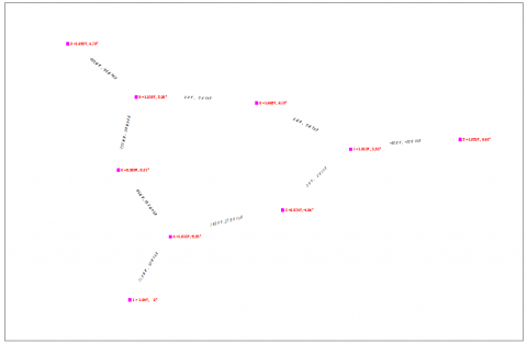
Figure 2. A directed graph plot of the system obtained from Newton Raphson’s solution (1)
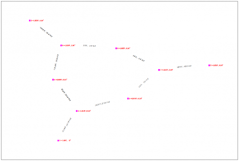
Figure 3. A directed graph plot of the system obtained from Newton Raphson’s solution (2)
Table 7. Line flow and losses of IEEE 9-bus system obtained from Newton Raphson
|
Line Flow and Losses |
|||||
|
Line |
Line Flow |
Line Loss |
|||
|
From Bus (f) |
To Bus (t) |
A (MW) |
B (Mvar) |
MW |
Mvar |
|
1 |
4 |
71.945 |
50.044 |
0.000 |
4.090 |
|
4 |
5 |
41.086 |
33.095 |
0.000 |
-14.514 |
|
4 |
6 |
30.859 |
12.859 |
0.231 |
-14.590 |
|
6 |
9 |
-59.371 |
-2.551 |
1.405 |
2.516 |
|
5 |
7 |
-84.251 |
-2.391 |
2.394 |
9.023 |
|
9 |
3 |
-85.000 |
-8.363 |
0.000 |
4.117 |
|
7 |
2 |
-163.000 |
-11.531 |
0.000 |
16.265 |
|
9 |
8 |
24.223 |
3.296 |
0.090 |
-20.589 |
|
7 |
8 |
76.355 |
0.118 |
0.488 |
-10.997 |
|
Total Loss |
|
|
|
4.608 |
-24.679 |
Table 8. Line flow and losses of IEEE 9-bus system obtained from Gauss Seidel
|
Line Flow and Losses |
|||||
|
Line |
Line Flow |
Line Loss |
|||
|
From Bus (f) |
To Bus (t) |
A (MW) |
B (Mvar) |
MW |
Mvar |
|
1 |
4 |
74.945 |
49.749 |
0.000 |
4.298 |
|
4 |
5 |
42.319 |
32.892 |
0.346 |
-14.454 |
|
4 |
6 |
31.806 |
12.714 |
0.239 |
-14.549 |
|
6 |
9 |
-58.618 |
-2.697 |
1.369 |
2.358 |
|
5 |
7 |
-83.248 |
-2.601 |
2.336 |
8.730 |
|
9 |
3 |
-84.162 |
-8.344 |
0.000 |
4.036 |
|
7 |
2 |
-162.088 |
-11.499 |
0.000 |
16.082 |
|
9 |
8 |
24.662 |
3.249 |
0.092 |
-20.571 |
|
7 |
8 |
76.139 |
0.183 |
0.485 |
-11.022 |
|
Total Loss |
|
|
|
4.867 |
-25.092 |
4.1.1 Comparison of the computational time, maximum power mismatch and the iteration number of the two methods
Table 9 presents the comparison of computational time, maximum power mismatch, and iteration number.
Table 9. Comparison of computational time, maximum power mismatch and iteration number
|
Newton Raphson |
Gauss Siedlel |
||||
|
Computational Time (s) |
Maximum power mismatch (MW) |
Iteration Number |
Computational Time (s) |
Maximum power mismatch (MW) |
Iteration Number |
|
$4 \times 10^{-3}$ |
4 |
7 |
$3 \times 10^{-3}$ |
0.0204582 |
11 |
4.1.2 Directed graph
This section presents the directed graph of the 9-bus system resolved from the NR and GS methods. It shows the node voltages and phase angle on each bus as well the real and reactive power loss on each transmission line. The pink dots represent the buses. The index of the bus is shown beside it. The lines represent the transmission line. The arrows represent the loads.
4.2 Discussion
4.2.1 Simulation results
The solutions to some required unknown variables obtained after using both load flow methods are shown in Tables 5 and 6 for the NR and GS methods, respectively. When the values from the two tables are compared, there are minor differences between them. This difference isn't all that significant. This demonstrates that the two methods produce roughly comparable results (as shown from the total load and generation power).
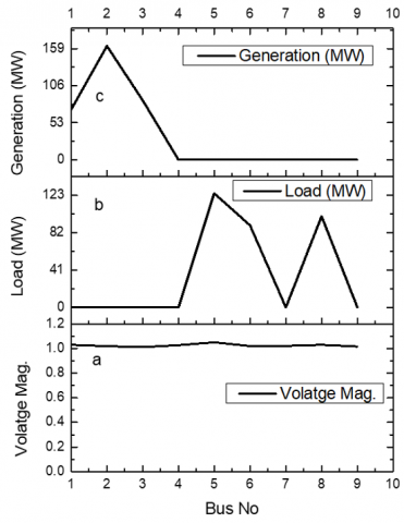
Figure 4. Multiple graphs of the voltage magnitude, load power and generation power on each bus for the IEEE 9 bus system obtained from Newton Raphson’s solution
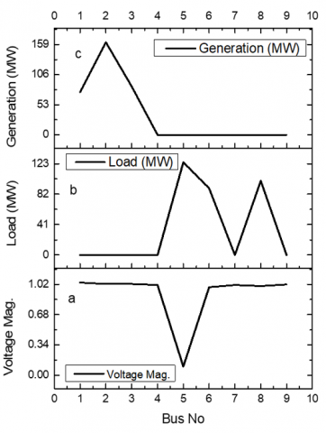
Figure 5. Graph of the voltage magnitude, load power and generation power on each bus for the IEEE 9 bus system obtained from Newton Raphson’s solution
Figure 4 depicts the generation and load power, as well as the voltage magnitude on each bus, as calculated using Newton Raphson's power flow solution. Figure 5 depicts the same plot, but for the Gauss Seidel's power flow solution. The two figures show that the voltage magnitude in bus 5 of the GS solution is significantly lower or attenuated when compared to the NS solution.
4.2.2 Line flow and line losses
In the domain of power system analysis, understanding how electricity moves and where energy is lost in a power system is essential for keeping things running smoothly. Using the Gauss-siedel and Newton-Raphson methods, the line flows and losses are derived from the solution data yielded from the load flow solutions of each of these numerical methods.
By using the results from the power analysis, the line current flowing in different parts of the system can be determined using the famous Ohm’s law equation:
$I=\frac{S}{V}$ (26)
where,
I-Line Current,
V-Voltage Magnitude,
S-Apparent Power.
The apparent power underscores the interplay of electrical magnitudes.
$S=A+j B$ (27)
By utilizing the voltage magnitudes and angles from the result of power flow analysis from the two methods, line currents are carefully calculated iteratively for each transmission line.
Line power flows show how electricity is moving between places. It is a pivotal metric for line performance. To calculate this, we look at the voltage and the current, and do some math to see how much power is moving around. With this information, we can see which parts of the system are busy and which ones might need attention.
The magnitude of line power flow is established as the product of the sending-end voltage, the conjugate of the line current:
$S=V_i * I^*$ (28)
By applying this equation in conjunction with voltage magnitudes and calculated line currents, the real-time assessment of power propagation becomes discernible for every transmission line.
Incorporating the concept of power losses adds depth to power system evaluations. Real and reactive power losses manifest as outcomes of line current interaction with line resistances and reactances, respectively by employing the following expressions:
A_loss $=\mathrm{I}^2 * \mathrm{R}$ (29)
B_loss $=\mathrm{I}^2 * \mathrm{X}$ (30)
where,
I-Line Current, R-Resistance of transmission line, X-Reactance of transmission line, A_loss-Real Power Loss, B_loss-Reactive Power Loss.
By conducting this analysis, a more profound comprehension of energy dissipation arises, facilitating the efficient administration and enhancement of the power distribution system.
The knowledge acquired from computing line flows and losses through the application of the Newton-Raphson and Gauss-Seidel techniques has significant implications for both power system analysis and operation. Through a comprehensive understanding of current distribution, apparent power, and energy losses, engineers and analysis can anticipate congestion points in advance, optimize power transmission processes, and improve network stability.
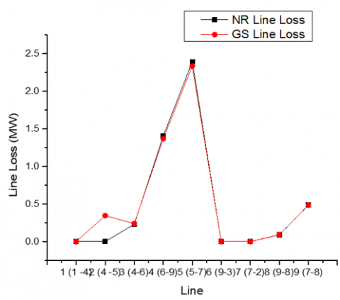
Tables 6 and 7 show the line flow and losses on each bus system line obtained from the nr and gs power flow solutions. Figure 4 depicts the line loss resulting from the ns and gs solutions. The nr method clearly shows that line 2 of the bus system (the line connecting buses 4 and 5) has a significant drop when compared to the gs method.
4.2.3 Tolerance
In the realm of power system analysis utilizing numerical methods such as Newton-Raphson and Gauss-Seidel, convergence refers to the attainment of a stable and precise solution. The determination of convergence hinges upon meeting specific criteria, which are evaluated by assessing tolerance-a pivotal parameter that significantly influences these criteria.
The Newton-Raphson method uses iterative corrections to improve the accuracy of calculated values of bus voltages and angles. Accuracy is influenced by initial guesses and convergence criteria set for maximum change in bus voltage magnitudes and angles. Lower tolerance values result in higher accuracy, but setting it too low may increase computational time without significant improvement.
Similar to the Newton-Raphson procedure, precision in Gauss-Seidel is impacted by the convergence criteria. Decreasing tolerance values result in more precise solutions, but akin to Newton-Raphson, excessively low tolerance settings may cause excessive computational time without significant improvements in accuracy.
The simulation's tolerance iteration value was set to 0.001. This means that using a high tolerance value for such analysis increased the accuracy of the solution.
4.2.4 Computational time
Table 8 shows the computation time for load flow solutions using a selected iteration value of 0.001 for the NR and GS methods. For the 9-bus system, the computational time for the GS and NR methods is very similar.
4.2.5 Convergence
Convergence is used to calculate how quickly a power flow arrives at its solution. The rate of convergence is calculated by graphing the maximum power mismatch versus the number of iterations.
Newton-Raphson convergence is based on the max change in voltage magnitudes/angles. If the change is below tolerance, it has converged. A smaller tolerance means tighter convergence, more iterations, and better accuracy.
Gauss-Seidel checks convergence by comparing new and old voltage values. Lower tolerance means stricter convergence but longer computation.
When compared to the Newton-Raphson method, the Gauss-Seidel method has a slower convergence rate. Newton Raphson has the fastest convergence rate. The results of the line graph of the line flow and line loss in the different lines of the IEEE 9-bus system are presented in Figure 6.
Figure 6. Line graph of the line flow and line loss in the different lines of the IEEE 9-bus system
Both Newton-Raphson and Gauss-Seidel methods have been extensively studied for their convergence behavior in load flow analysis. Understanding convergence behavior has led to more robust and reliable power system analysis tools.
Investigations have shown that both methods can provide accurate results when applied correctly. However, the choice of method, initial conditions, and convergence criteria can impact accuracy.
Comparisons of the Newton-Raphson and Gauss-Seidel methods have also revealed the differences in computational efficiency. Gauss-Seidel is simpler but may require more iterations, while Newton-Raphson can converge faster but involves more complex calculations. These findings have guided the selection of methods based on the size and complexity of the power system.
The study found that computational/numerical methods can be used to calculate line flows and power losses in a power system. These methods derive the voltage magnitude, phasal angles, real and reactive power of the system's buses. The load flow analysis methods of Gauss Seidel and Newton Raphson were used to analyze an IEEE 9-bus test system, with results showing only slight differences between the total line flow and losses obtained from the two iterative solutions. A complete load flow analysis was performed on an IEEE standard 9-bus system using both computational methods.
[1] Vijayvargia, A., Jain, S., Meena, S., Gupta, V., Lalwani, M. (2016). Comparison between different load flow methodologies by analyzing various bus systems. International Journal of Electrical Engineering, 9(2): 127-138.
[2] Xi-Fang, W., Yonghua, S., Malcolm, I. (2008). Modern power system analysis. New York: Springer Science+Business Media. https://doi.org/10.1007/978-0-387-72853-7
[3] Hale, H.W., Goodrich, R.W. (1959). Digital computation or power flow-some new aspects. Transactions of the American Institute of Electrical Engineers. Part III: Power Apparatus and Systems, 78(3): 919-923. https://doi.org/10.1109/AIEEPAS.1959.4500466
[4] Grainger, J.J., Stevenson Jr, W.D. (1994). Power system analysis. McGraw-Hill Series in Electrical and Computer Engineering.
[5] Kabisama, H. (1993). Electrical power engineering. New York: McGraw-Hill.
[6] Milano, F. (2008). Continuous Newton's method for power flow analysis. IEEE Transactions on Power Systems, 24(1): 50-57. https://doi.org/10.1109/TPWRS.2008.2004820
[7] Hadi, S. (2010). Power system analysis (3rd ed.). Edition, New York: Mc-Graw Hill.
[8] Keyhani, A., Abur, A., Hao, S. (1989). Evaluation of power flow techniques for personal computers. IEEE Transactions on Power Systems, 4(2): 817-826. https://doi.org/10.1109/59.193857
[9] Aroop, B., Satyajit, B., Sanjib, H. (2014). Power flow analysis on IEEE 57 bus system using Mathlab. International Journal of Engineering Research & Technology (IJERT), 3.
[10] Adejumobi, I.A., Adepoju, G.A., Hamzat, K.A., Oyeniran, O.R. (2014). Numerical methods in load flow analysis: An application to Nigeria grid system. International Journal of Electrical and Electronics Engineering (IJEEE), 3.
[11] Gilbert, G.M., Bouchard, D.E., Chikhani, A.Y. (1998). A comparison of load flow analysis using distflow, gauss-seidel, and optimal load flow algorithms. In Conference Proceedings. IEEE Canadian Conference on Electrical and Computer Engineering (Cat. No. 98TH8341), 2: 850-853. https://doi.org/10.1109/CCECE.1998.685631
[12] Afolabi, O.A., Ali, W.H., Cofie, P., Fuller, J., Obiomon, P., Kolawole, E.S. (2015). Analysis of the load flow problem in power system planning studies. Energy and Power Engineering, 7(10): 509. http://dx.doi.org/10.4236/epe.2015.710048
[13] Aeggegn, D.B., Salau, A.O., Gebru, Y.W., Agajie, T. (2022). Mitigation of reactive power and harmonics in a case of industrial customer. International Journal of Engineering Research in Africa, 60: 107-124. https://doi.org/10.4028/p-j716jb
[14] Kassahun, H.E., Salau, A.O., Osaloni, O.O., Olaluyi, O.J. (2023). Power system small signal stability enhancement using fuzzy based statcom. Przeglad Elektrotechniczny, 2023(8): 27-32. https://doi.org/10.15199/48.2023.08.05
[15] Alyu, A.B., Salau, A.O., Khan, B., Eneh, J.N. (2023). Hybrid GWO-PSO based optimal placement and sizing of multiple PV-DG units for power loss reduction and voltage profile improvement. Scientific Reports, 13(1): 6903. https://doi.org/10.1038/s41598-023-34057-3
[16] Gebru, F.M., Salau, A.O., Mohammed, S.H., Goyal, S.B. (2022). Analysis of 3-phase symmetrical and unsymmetrical fault on transmission line using Fortescue Theorem. WSEAS Transactions on Power Systems, 17: 316-323. https://doi.org/10.37394/232016.2022.17.32