Mohammad A. Gharaibeh
© 2022 IIETA. This article is published by IIETA and is licensed under the CC BY 4.0 license (http://creativecommons.org/licenses/by/4.0/).
OPEN ACCESS
This paper uses the finite difference method (FDM) to provide a high-accuracy numerical approach to solve for the governing equations of two elastically coupled plates under symmetrical bending. The solution strategy, including governing equations and boundary conditions, is thoroughly discussed, and presented. Finally, this solution was used to test the effect of the key parameters of the coupled plates structure on the mechanical response of the system and relate that to the reliability performance of electronic packages under mechanical bending.
elastically coupled plates, finite difference methods, mathematical representation, electronic assemblies, solder joints, mechanical bending
The problem of the two elastically coupled, i.e., joined, beams and/or plates repetitively appears in real-life structures such as railways, engineering structures, and electronics [1, 2]. For the buildings and engineering structures, such beams are called composite beams and commonly joined together using epoxy resins [3, 4]. In electronic industries, a classic electronic package is usually made of a printed circuit board (PCB) that is connected to an integrated component (IC) using an array of solder interconnects. As electronics are progressively subjected to mechanical failures due to various static and dynamic loadings [5, 6], the reliability assessment of electronic assemblies has become a major interest of research studies in literature [7, 8]. Particularly, the coupled beams problem was much analytically investigated more than the coupled plates problem due to problem simplicity and less complexity. In the elastically attached beams model, the PCB and the IC are treated as two beams, both are based Euler-Bernoulli theory, and the solder joints are as an elastic layer composed of finite number of axial springs. For the analytical research works on this problem, Wong [9] formulated a closed-form analytical model to compute the deformations of the coupling layer and this was related to the solder deflections and hence stresses. Wong et al. [10-13] have developed several solutions of the coupled beams under bending system, in which both axial and flexural deformations of the elastic layer were considered. Engle [14] and Pitarresi and Ceurter [15] created the analytical solution of the coupled beams with a centrally applied point force problem and computed solder stresses accordingly. Gharaibeh et al. [16] extended the solution of Pitarresi and used it to solve for the problem of the partially coupled elastic beams structure and validated that later with experimental data [17]. Recently, Gharaibeh et al. [18] used finite difference method (FDM) to numerically solve for the symmetric bending of two coupled beams problem and the results of this numerical solution were validated with finite element analysis (FEA) data.
For the two elastically coupled plate bending problem, only a few works are available in literature. In this model, the PCB and the integrated circuit package are both considered as two elastic rectangular isotropic plates that are joined together using a finite number of axial springs, i.e., solders, array. The first introduction of the two coupled plates structure was in 2015 where Gharaibeh et al. [19] used Ritz method to solve for the free vibration characteristics of the problem and computed the natural frequencies and mode shapes of the coupled plates system. Later, Gharaibeh et al. [20-23] expanded this solution to solve for the forced vibrations of the coupled plates due to harmonic [20, 21], transient [22], and random vibrations excitations [23]. In all works, the solution was validated with experiments and thus employed to test the influence of the geometric and material parameters of the structure on solder joints deflections, strains, and stresses.
The main goal of the current paper is to revisit the problem of the two elastically coupled plates and employ the finite difference method to solve the governing partial differential equations (PDE) of the system and hence compute the elastic coupling layer axial deformations. This numerical solution was then used to explore the effect of the various key material and geometric structural parameters of the electronic assembly on the expected solder stresses. The originality and the main value of this approach is that it can be easily modified and hence generalized to solve several loading and boundary conditions that could be imposed on two coupled plates structure.
The organization of this paper starts by a detailed description of the coupled plates problem including the governing equations as well as the imposed boundary and loading conditions. The details of the implementation of the finite difference method in solving the governing equations was fully presented. Finally, the results of this solution are provided and thoroughly discussed.
2.1 Elastically coupled plates problem details
2.1.1 Problem definition
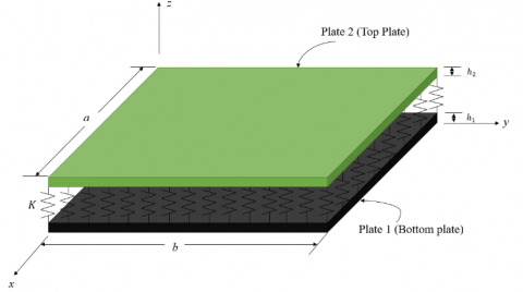
As described earlier, the two elastically coupled plates under bending problem is mainly directed towards the electronic packaging application. In this model, the board and the package are designated as thin elastic rectangular plates, and both plates are elastically connected by an evenly distributed matrix of linear axial springs, i.e., solder interconnects. Considering Figure 1, the IC package is plate 1 and the PCB is plate 2. The current work is limited for the case of plate 1 and plate 2 are equal in length (a) and width (b). The thickness of plate 1 is (h1) and plate 2 is (h2). The bending, i.e., flexural, rigidity of plate 1 and plate 2 are D1 and D2, respectively. If the modulus of elasticity of a plate material is (E) and its Poisson’s ratio is (v), then the flexural rigidity is $D=\frac{E h^3}{12\left(1-v^2\right)}$. Hereinafter, the subscript 1 is used for plate 1 material and geometry (E1 and h1) and subscript 2 is for plate 2 characteristics (E2 and h2). Also, the deflection function of plate 1 is u1(x, y) and plate 2 deflection is u2(x, y).
Figure 1. Two elastically-coupled plates system details
2.1.2 Governing equations
The governing equations of the two coupled plates system with axial linear springs can be expressed as [19]:
$D_1 \nabla^{2 u_1}=K \delta(x, y)$
$D_2 \nabla^2 u_2=-K \delta(x, y)$ (1)
where, $\nabla^2=\frac{\partial^4}{\partial x^4}+\frac{\partial^4}{\partial x^2 \partial y^2}+\frac{\partial^4}{\partial y^4}$ is the biharmonic operator; δ(x, y) is the elastic layer transverse deflections. Generally, δ(x, y) is computed as the difference between plate 1 and plate 2 out-of-plane deflections, mathematically:
$\delta(x, y)=u_2(x, y)-u_1(x, y)$ (2)
By applying the biharmonic operator differentials in Eq. (2), thus:
$\nabla^2 \delta(x, y)=\nabla^2 u_2(x, y)-\nabla^2 u_1(x, y)$ (3)
By combining Eq. (3) and Eq. (1), the governing equation of the elastic layer deflection is:
$\nabla^2 \delta(x, y)+4 \alpha_1^4 \delta(x, y)=0$ (4)
where, $4 \alpha_1^4=K\left(\frac{1}{D_2}+\frac{1}{D_1}\right)$.
2.1.3 Boundary conditions
In mechanics, boundary and loading conditions play an essential rule in computing the mechanical behavior of the structural problem. In the present work, both plates are simply supported along all four edges. In such conditions, the plate deformations are restricted in the transverse direction, but the rotations are allowed. For the loadings, an external coupling moment (Ma) is applied along the opposite plate edges (x=0, y=a and x=b, y=a). Therefore, the problem boundary conditions can be written as:
For plate 1:
$u_1(0, y)=u_1(a, y)=u_1(x, 0)=u_1(x, b)=0$
$\frac{d^2 u_1}{d x^2}(x=0)=\frac{M_a}{D_1}$
$\frac{d^2 u_1}{d x^2}(x=a)=\frac{M_a}{D_1}$
$\frac{d^2 u_1}{d y^2}(y=0)=0$
$\frac{d^2 u_1}{d y^2}(y=b)=0$ (5)
For plate 2:
$u_2(0, y)=u_2(a, y)=u_2(x, 0)=u_2(x, b)=0$
$\frac{d^2 u_2}{d x^2}(x=0)=\frac{M_a}{D_2}$
$\frac{d^2 u_2}{d x^2}(x=a)=\frac{M_a}{D_2}$
$\frac{d^2 u_2}{d y^2}(y=0)=0$
$\frac{d^2 u_2}{d y^2}(y=b)=0$ (6)
Considering Eq. (2), the boundary conditions for δ(x,y), are
$\delta(0, y)=u_2(0, y)-u_1(0, y)=0$
$\delta(a, y)=u_2(a, y)-u_1(a, y)=0$
$\delta(x, 0)=u_2(x, 0)-u_1(x, 0)=0$
$\delta(x, b)=u_2(x, b)-u_1(x, b)=0$
$\frac{d^2 \delta(0, y)}{d x^2}=\frac{d^2 u_2(0, y)}{d x^2}-\frac{d^2 u_1(0, y)}{d x^2}$
$=M_a\left(\frac{1}{D_2}-\frac{1}{D_1}\right)$
$\frac{d^2 \delta(a, y)}{d x^2}=\frac{d^2 u_2(a, y)}{d x^2}-\frac{d^2 u_1(a, y)}{d x^2}$
$=M_a\left(\frac{1}{D_2}-\frac{1}{D_1}\right)$
$\frac{d^2 \delta(x, 0)}{d y^2}=\frac{d^2 u_2(x, 0)}{d y^2}-\frac{d^2 u_1(x, 0)}{d y^2}=0$
$\frac{d^2 \delta(x, b)}{d y^2}=\frac{d^2 u_2(x, b)}{d y^2}-\frac{d^2 u_1(x, b)}{d y^2}=0$ (7)
2.2 Finite difference method solution
2.2.1 Mathematical implementation
In this work, the finite difference method (FDM) was elected to solve for the elastic layer out-of-plane deformations. In this solution, Newton’s finite divided differences (FDD’s) are chosen to be substituted in the PDE of Eq. (4). Therefore, these differential equations would be transformed into a system of linear algebraic equations which can be solved conveniently. Before getting into the FDM details, the PDE of Eq. (4) is of the fourth order. Thus, an order reduction is required. This reduction will result into s system of two ordinary differential equations (ODE’s). this system of ODE’s is ready to be tackled using the FDM method. The order reduction process is done by letting v(x)=$d^2 \delta / d x^2+d^2 \delta / d y^2$, thus Eq. (4) can now be represented as pair of second order ODE’s as:
$v(x, y)=\frac{d^2 \delta}{d x^2}+\frac{d^2 \delta}{d y^2}$
$\frac{d^2 v}{d x^2}+\frac{d^4 v}{d y^4}=-4 \alpha_1^4 \delta(x, y)$ (8)
For the second derivatives terms of Eq. (8) above $d^2 v / d x^2, d^2 v / d y^2, d^2 \delta / d x^2$ and $d^2 \delta / d y^2$, the Newton’s FDD’s are:
$\frac{d^2 v}{d x^2}=\frac{v_{i+1, j}-2 v_{i, j}+v_{i-1, j}}{(\Delta x)^2}$
$\frac{d^2 v}{d y^2}=\frac{v_{i, j+1}-2 v_{i, j}+v_{i, j-1}}{(\Delta y)^2}$
$\frac{d^2 \delta}{d x^2}=\frac{\delta_{i+1, j}-2 \delta_{i, j}+\delta_{i-1, j}}{(\Delta x)^2}$
$\frac{d^2 \delta}{d y^2}=\frac{\delta_{i, j+1}-2 \delta_{i, j}+\delta_{i, j-1}}{(\Delta y)^2}$ (9)
where, Δx and Δy are the step size in the x and y directions, respectively; and i=0, 1, 2, …, n-1 , j=0, 1, 2, …, n-1 where n is the total number of nodes used in the FDM in x and y directions, respectively. Thus, $\Delta x=\frac{a}{n-1}, \Delta y=\frac{b}{n-1}$.
Therefore, the substitution of the FDD’s of Eq. (9) into the system shown in Eq. (8) gives the set of equations presented in Eq. (10).
It is important here to emphasize that the equations above (Eq. (10)) will end up in a system of 2*(N-2)2 tridiagonal algebraic linear equations as the exterior nodes (first and last nodes) are naturally satisfied by the boundary conditions of the problem. Where the interior nodes solutions needs to be calculated and this is the whole idea of FDM. The equations above apply for each of the interior nodes (N) of v(x, y) and δ(x,y), as the first and the last nodes, i.e., the exterior nodes, are normally specified by the boundary conditions. Such systems are simple and computationally effective to solve. An illustrative example on the use of FDM in solving Eq. (4) is thoroughly presented in Appendix A.
$(\Delta y)^2 v_{i+1, j}-2(\Delta y)^2 v_{i, j}+(\Delta y)^2 v_{i-1, j}+(\Delta x)^2 v_{i, j+1}-2(\Delta x)^2 v_{i, j}+(\Delta x)^2 v_{i, j-1}=-4 \alpha_1^4(\Delta x)^2(\Delta y)^2 \delta_i$
$(\Delta y)^2 \delta_{i+1, j}-2(\Delta y)^2 \delta_{i, j}+(\Delta y)^2 \delta_{i-1, j}+(\Delta x)^2 \delta_{i, j+1}-2(\Delta x)^2 \delta_{i, j}+(\Delta x)^2 \delta_{i, j-1}=(\Delta x)^2(\Delta y)^2 v_i$ (10)
2.2.2 Numerical accuracy study
Like any other numerical method, the accuracy of the FDM is highly dependable of the number of approximations, i.e., nodes, used in the solution. In fact, the more nodes considered is the more accurate but slower solution. Thus, a numerical accuracy check is required here and therefore, performed. In other words, the current numerical solution is optimized in terms of accuracy and computational efficiency. Therefore, several number of nodes (approximations) were considered. The elastic coupling layer deflections were computed for each approximation and recorded. Specifically, the deflections across the layer diagonal i.e., δ(x=y), were considered. During the process, the structural parameter used here are a=1, b=1, D1=1, D2=2, K=100 and Ma=1.
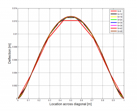
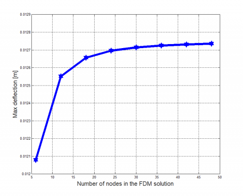
Figure 2 shows the deflections across the layer diagonal for each tested configuration and Figure 3 presents the corresponding maximum diagonal deflections. In both figures N is the number of interior nodes in the FDM solutions (remember N=n-2 where n is the total number of nodes). The results of this accuracy check suggests that for N=30 nodes the deflections have reached a converged numerical value. Thus, this number of nodes was selected to conduct the rest of the numerical analysis of this present study.
Figure 2. Numerical accuracy check: Elastic layer deformations across the diagonal for several mesh configurations
Figure 3. Numerical accuracy check: Elastic layer maximum deformations for several mesh configurations
This study presents the effect of the key structural parameters of the coupled plate configuration on solder deflection. During this analysis, one key parameter was varied at a time while all other factors are held constant. Additionally, unless otherwise mentioned, for generalization a unity value was used for the geometric and/or material parameter as D1=1 N.m, D2=1 N.m, K=100 N/m3, a=1 m and b=1 m. Also, the analysis was carried out for a unity applied coupling moment Ma=1 N.m.
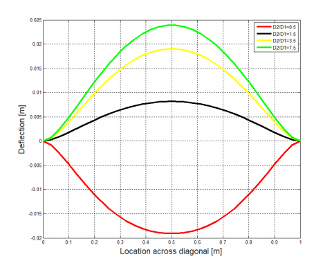
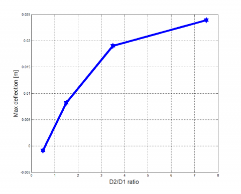
In practice, it is mighty believed that the relative rigidity between the IC package and the PCB board (D2/D1 ratio) has a dominant and major effect on the solder interconnect deformations, and thus, stresses. The current paper studied this effect by varying the D2/D1 ratio while keeping the stiffness of the coupling layer constant. Figure 4 depicts the elastic layer deflections across the diagonal of the plate structure. The corresponding maximum deflections as a function of the D2/D1 ratio are also available in Figure 5. The first observation that can be made here is that, for all D2/D1 values, the maximum deflections of the elastic layer are at the center of the layer (Figure 4). Also, for D2/D1 less than 1 (stiffer IC package), the elastic layer is under compression as the deformations are negative. Furthermore, for D2/D1 larger than 1 (stiffer board), the layer is undergoing tensile deformations as the deflections are positive. Additionally, as D2/D1 increases, or the relative rigidity between the two plates becomes greater, larger coupling layer deflections are expected (Figure 5). By relating that to the solder interconnects, for larger difference in relative stiffness between the PCB and the component, shorter solder fatigue life is anticipated.
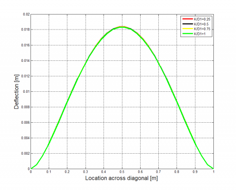
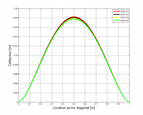
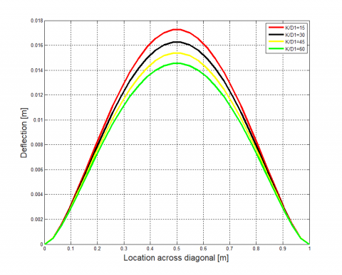
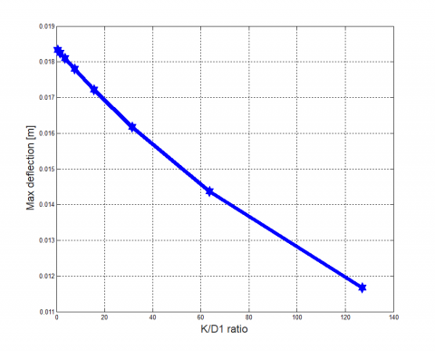
The second important structural factor that affects the elastic coupling layer behavior is the relative stiffness between the elastic layer and either one of the plates. In the current work, relative stiffness between the layer and plate 1, or K/D1 ratio, was selected. Figure 6 shows the elastic layer deformations across the diagonal of the layer for different K/D1 ratio values. This effect was studied at three scales. The first scale is for a very compliant layer (K/D1 less than 1), as shown in Figure 6 (a). the second is for stiffer layer (K/D1 is greater than 1 but less than 10), this case is presented in Figure 6 (b). The third and last scale is for very stiff layer (K/D1 is greater than 10), which is available in Figure 6 (c). The result show that generally for stiffer layer, i.e., solders, the deformations are smaller and hence longer solder fatigue life. However, for this effect to be significant, the change in the relative stiffness must be quite large. For a closer look on this effect, the layer maximum deflections, the deflections at the center of the layer, versus the K/D1 ratio is plotted in Figure 7.
Figure 4. Elastic layer deformations across the diagonal for several D2/D1 ratios
Figure 5. Elastic layer maximum deformations versus D2/D1 ratio
(a) K/D1 less than 1
(b) 1<K/D1<10
(c) K/D1 greater than 10
Figure 6. Elastic layer deformations across the diagonal for several K/D1 ratio
Figure 7. Elastic layer maximum deformations versus K/D1 ratio
This figure confirms the previous conclusions, the stiffer the layer the smaller the deformations. However, this effect is minor. Specifically, when K/D1 is equal to 0.25 the layer maximum deflection is 18.5 $\mu m$ while the maximum deflection is equal to 11.7 $\mu m$ when K/D1=125. Thus, to reduce the elastic layer deflections by almost 37% the relative stiffness between the layer and plate 1 must increase by 500 times. Therefore, this effect is considered to be minor as it is practically impossible to achieve this value of relative stiffness.
The third and last geometric parameter studied in the present work is the effect of the plate aspect ratio, i.e., the ratio between the plate length and width (a/b) on the coupling layer out-of-plane deformations.
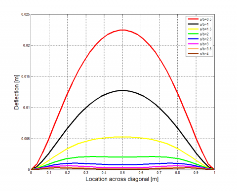
Figure 8 shows this effect. For small a/b values, larger elastic layer deflections are anticipated and the deformations across the diagonal are in a curved shape. However, for smaller aspect ratios, smaller layer deflections are expected and the deformations across the layers’ diagonal are flat as the structure becomes very stiff which prohibits the deformations.
Figure 8. Elastic layer deformations across the diagonal for several plate aspect (a/b) ratio
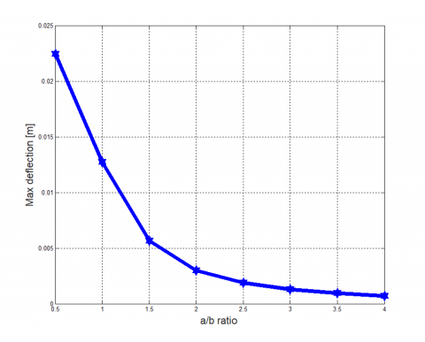
Additionally, as shown in Figure 9, the aspect ratio effect is more dominant for smaller ratios (a/b less than 2) and it becomes less significant for larger plate sizes.
Figure 9. Elastic layer maximum deformations versus plate aspect (a/b) ratio
The finite difference method was employed to solve for the two elastically coupled under symmetrical bending problem. During the solution, the fourth order partial differential equations that governs the system was transformed into two second order equations and hence the finite difference method was applied. The numerical efficiency of this method was explicitly ensured. Finally, the influence of the key structural geometric and material parameters was thoroughly tested and hence discussed with special attention to its application in the mechanical analysis of electronic assemblies under bending.
The authors wish to thank the deanship of scientific research at the Hashemite University for providing the necessary tools and funds. In addition, we would like to acknowledge Mr. Sufian Almitwali of the mechanical engineering department of the Hashemite University for their good help throughout this work in the generation of the MATLAB figures.
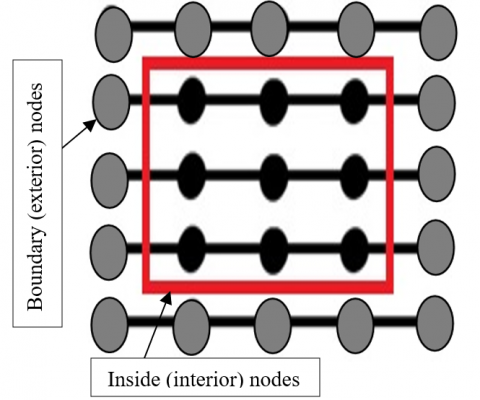
The details of the implementation of the FDM method are shown in this appendix with an interpretative example. In this example, 5 nodes along each side in the x and y-directions are considered as shown in Figure A.1.
Figure A.1. FDM representation: Five nodes per axis
The nodes were named as (i,j) where i is the node number along the x-axis and j is along the y-axis. Each index is numbered from 0 to 4. The resultant number of nodes is 25 where 16 of them are spotted at the boundaries of the structural and called as the exterior nodes. The remaining 9 nodes are called the interior nodes as they are located inside the structure. The values of v(x,y) at the exterior or boundary nodes are naturally obtained considering the BC’s of Eq. (5) as well as Eq. (6) and Eq. (7), as
$v_{0,0}=v(0,0)=\frac{d^2 \delta(0,0)}{d x^2}+\frac{d^2 \delta(0,0)}{d y^2}=M_a\left(\frac{1}{D_2}-\frac{1}{D_1}\right)$
$v_{0,1}=v(0,1)=\frac{d^2 \delta(0,1)}{d x^2}+\frac{d^2 \delta(0,1)}{d y^2}=M_a\left(\frac{1}{D_2}-\frac{1}{D_1}\right)$
$v_{0,2}=v(0,2)=\frac{d^2 \delta(0,2)}{d x^2}+\frac{d^2 \delta(0,2)}{d y^2}=M_a\left(\frac{1}{D_2}-\frac{1}{D_1}\right)$
$v_{0,3}=v(0,3)=\frac{d^2 \delta(0,3)}{d x^2}+\frac{d^2 \delta(0,3)}{d y^2}=M_a\left(\frac{1}{D_2}-\frac{1}{D_1}\right)$
$v_{0,4}=v(0,4)=\frac{d^2 \delta(0,4)}{d x^2}+\frac{d^2 \delta(0,4)}{d y^2}=M_a\left(\frac{1}{D_2}-\frac{1}{D_1}\right)$
$v_{4,0}=v(4,0)=\frac{d^2 \delta(4,0)}{d x^2}+\frac{d^2 \delta(4,0)}{d y^2}=M_a\left(\frac{1}{D_2}-\frac{1}{D_1}\right)$
$v_{4,1}=v(4,1)=\frac{d^2 \delta(4,1)}{d x^2}+\frac{d^2 \delta(4,1)}{d y^2}=M_a\left(\frac{1}{D_2}-\frac{1}{D_1}\right)$
$v_{4,2}=v(4,2)=\frac{d^2 \delta(4,2)}{d x^2}+\frac{d^2 \delta(4,2)}{d y^2}=M_a\left(\frac{1}{D_2}-\frac{1}{D_1}\right)$
$v_{4,3}=v(4,3)=\frac{d^2 \delta(4,3)}{d x^2}+\frac{d^2 \delta(4,3)}{d y^2}=M_a\left(\frac{1}{D_2}-\frac{1}{D_1}\right)$
$v_{4,4}=v(4,4)=\frac{d^2 \delta(4,4)}{d x^2}+\frac{d^2 \delta(4,4)}{d y^2}=M_a\left(\frac{1}{D_2}-\frac{1}{D_1}\right)$
$v_{1,0}=v(1,0)=\frac{d^2 \delta(1,0)}{d x^2}+\frac{d^2 \delta(1,0)}{d y^2}=0$
$v_{2,0}=v(2,0)=\frac{d^2 \delta(2,0)}{d x^2}+\frac{d^2 \delta(2,0)}{d y^2}=0$
$v_{3,0}=v(3,0)=\frac{d^2 \delta(3,0)}{d x^2}+\frac{d^2 \delta(3,0)}{d y^2}=0$
$v_{0,4}=v(0,4)=\frac{d^2 \delta(0,4)}{d x^2}+\frac{d^2 \delta(0,4)}{d y^2}=M_a\left(\frac{1}{D_1}-\frac{1}{D_2}\right)$
$v_{1,4}=v(1,4)=\frac{d^2 \delta(1,4)}{d x^2}+\frac{d^2 \delta(1,4)}{d y^2}=0$
$v_{2,4}=v(2,4)=\frac{d^2 \delta(2,4)}{d x^2}+\frac{d^2 \delta(2,4)}{d y^2}=0$
$v_{3,4}=v(3,4)=\frac{d^2 \delta(3,4)}{d x^2}+\frac{d^2 \delta(3,4)}{d y^2}=0$ (A1)
Also, the values of δ(x) at the boundary nodes are given by
$\delta_{0,0}=\delta(0,0)=0$
$\delta_{0,1}=\delta(0,1)=0$
$\delta_{0,2}=\delta(0,2)=0$
$\delta_{0,3}=\delta(0,3)=0$
$\delta_{0,4}=\delta(0,4)=0$
$\delta_{4,0}=\delta(4,0)=0$
$\delta_{4,1}=\delta(4,1)=0$
$\delta_{4,2}=\delta(4,2)=0$
$\delta_{4,3}=\delta(4,3)=0$
$\delta_{4,4}=\delta(4,4)=0$
$\delta_{1,0}=\delta(1,0)=0$
$\delta_{2,0}=\delta(2,0)=0$
$\delta_{3,0}=\delta(3,0)=0$
$\delta_{1,4}=\delta(1,4)=0$
$\delta_{2,4}=\delta(2,4)=0$
$\delta_{3,4}=\delta(3,4)=0$ (A2)
For the remaining and the unknown interior 9 nodes, two equations, one for v(x,y) and one for δ(x,y), are required and hence formulated for each. Thus, 18 linear algebraic equations are derived considering Eq. (10), so.
|
$i=1$ $j=1$ |
$(\Delta y)^2 v_{2,1}-2(\Delta y)^2 v_{1,1}+(\Delta y)^2 v_{0,1}+(\Delta x)^2 v_{1,2}-2(\Delta x)^2 v_{1,1}+(\Delta x)^2 v_{1,0}=-4 \alpha_1^4(\Delta x)^2(\Delta y)^2 \delta_{1,1}$ |
(A3.1.a) |
|
|
$(\Delta y)^2 \delta_{2,1}-2(\Delta y)^2 \delta_{1,1}+(\Delta y)^2 \delta_{0,1}+(\Delta x)^2 \delta_{1,2}-2(\Delta x)^2 \delta_{1,1}+(\Delta x)^2 \delta_{1,0}=(\Delta x)^2(\Delta y)^2 v_{1,1}$ |
(A3.1.b) |
||
|
$i=1$ $j=2$ |
$(\Delta y)^2 v_{2,2}-2(\Delta y)^2 v_{1,2}+(\Delta y)^2 v_{0,2}+(\Delta x)^2 v_{1,3}-2(\Delta x)^2 v_{1,2}+(\Delta x)^2 v_{1,0}=-4 \alpha_1^4(\Delta x)^2(\Delta y)^2 \delta_{1,2}$ |
(A3.2.a) |
|
|
$(\Delta y)^2 \delta_{2,2}-2(\Delta y)^2 \delta_{1,2}+(\Delta y)^2 \delta_{0,2}+(\Delta x)^2 \delta_{1,3}-2(\Delta x)^2 \delta_{1,2}+(\Delta x)^2 \delta_{1,0}=(\Delta x)^2(\Delta y)^2 v_{1,2}$ |
(A3.2.b) |
||
|
$i=1$ $j=3$ |
$(\Delta y)^2 v_{2,3}-2(\Delta y)^2 v_{1,3}+(\Delta y)^2 v_{0,3}+(\Delta x)^2 v_{1,4}-2(\Delta x)^2 v_{1,3}+(\Delta x)^2 v_{1,2}=-4 \alpha_1^4(\Delta x)^2(\Delta y)^2 \delta_{1,3}$ |
(A3.3.a) |
|
|
$(\Delta y)^2 \delta_{2,3}-2(\Delta y)^2 \delta_{1,3}+(\Delta y)^2 \delta_{0,3}+(\Delta x)^2 \delta_{1,4}-2(\Delta x)^2 \delta_{1,3}+(\Delta x)^2 \delta_{1,2}=(\Delta x)^2(\Delta y)^2 v_{1,3}$ |
(A3.3.b) |
||
|
$i=2$ $j=1$ |
$(\Delta y)^2 v_{3,1}-2(\Delta y)^2 v_{2,1}+(\Delta y)^2 v_{1,1}+(\Delta x)^2 v_{2,2}-2(\Delta x)^2 v_{2,1}+(\Delta x)^2 v_{2,0}=-4 \alpha_1^4(\Delta x)^2(\Delta y)^2 \delta_{2,1}$ |
(A3.4.a) |
|
|
$(\Delta y)^2 \delta_{3,1}-2(\Delta y)^2 \delta_{2,1}+(\Delta y)^2 \delta_{1,1}+(\Delta x)^2 \delta_{2,2}-2(\Delta x)^2 \delta_{2,1}+(\Delta x)^2 \delta_{2,0}=(\Delta x)^2(\Delta y)^2 v_{2,1}$ |
(A3.4.b) |
||
|
$i=2$ $j=2$ |
$(\Delta y)^2 v_{3,2}-2(\Delta y)^2 v_{2,2}+(\Delta y)^2 v_{1,2}+(\Delta x)^2 v_{2,3}-2(\Delta x)^2 v_{2,2}+(\Delta x)^2 v_{2,1}=-4 \alpha_1^4(\Delta x)^2(\Delta y)^2 \delta_{2,2}$ |
(A3.5.a) |
|
|
$(\Delta y)^2 \delta_{3,2}-2(\Delta y)^2 \delta_{2,2}+(\Delta y)^2 \delta_{1,2}+(\Delta x)^2 \delta_{2,3}-2(\Delta x)^2 \delta_{2,2}+(\Delta x)^2 \delta_{2,1}=(\Delta x)^2(\Delta y)^2 v_{2,2}$ |
(A3.5.b) |
||
|
$i=2$ $j=3$ |
$(\Delta y)^2 v_{3,3}-2(\Delta y)^2 v_{2,3}+(\Delta y)^2 v_{1,3}+(\Delta x)^2 v_{2,4}-2(\Delta x)^2 v_{2,3}+(\Delta x)^2 v_{2,2}=-4 \alpha_1^4(\Delta x)^2(\Delta y)^2 \delta_{2,3}$ |
(A3.6.a) |
|
|
$(\Delta y)^2 \delta_{3,3}-2(\Delta y)^2 \delta_{2,3}+(\Delta y)^2 \delta_{1,3}+(\Delta x)^2 \delta_{2,4}-2(\Delta x)^2 \delta_{2,3}+(\Delta x)^2 \delta_{2,2}=(\Delta x)^2(\Delta y)^2 v_{2,3}$ |
(A3.6.b) |
||
|
$i=3$ $j=1$ |
$(\Delta y)^2 v_{4,1}-2(\Delta y)^2 v_{3,1}+(\Delta y)^2 v_{2,1}+(\Delta x)^2 v_{3,2}-2(\Delta x)^2 v_{3,1}+(\Delta x)^2 v_{3,0}=-4 \alpha_1^4(\Delta x)^2(\Delta y)^2 \delta_{3,1}$ |
(A3.7.a) |
|
|
$(\Delta y)^2 \delta_{4,1}-2(\Delta y)^2 \delta_{3,1}+(\Delta y)^2 \delta_{2,1}+(\Delta x)^2 \delta_{3,2}-2(\Delta x)^2 \delta_{3,1}+(\Delta x)^2 \delta_{3,0}=(\Delta x)^2(\Delta y)^2 v_{3,1}$ |
(A3.7.b) |
||
|
$i=3$ $j=2$ |
$(\Delta y)^2 v_{4,2}-2(\Delta y)^2 v_{3,2}+(\Delta y)^2 v_{2,2}+(\Delta x)^2 v_{3,3}-2(\Delta x)^2 v_{3,2}+(\Delta x)^2 v_{3,1}=-4 \alpha_1^4(\Delta x)^2(\Delta y)^2 \delta_{3,2}$ |
(A3.8.a) |
|
|
$(\Delta y)^2 \delta_{4,2}-2(\Delta y)^2 \delta_{3,2}+(\Delta y)^2 \delta_{2,2}+(\Delta x)^2 \delta_{3,3}-2(\Delta x)^2 \delta_{3,2}+(\Delta x)^2 \delta_{3,1}=(\Delta x)^2(\Delta y)^2 v_{3,2}$ |
(A3.8.b) |
||
|
$i=3$ $j=3$ |
$(\Delta y)^2 v_{4,3}-2(\Delta y)^2 v_{3,3}+(\Delta y)^2 v_{2,3}+(\Delta x)^2 v_{3,4}-2(\Delta x)^2 v_{3,3}+(\Delta x)^2 v_{3,2}=-4 \alpha_1^4(\Delta x)^2(\Delta y)^2 \delta_{3,3}$ |
(A3.9.a) |
|
|
$(\Delta y)^2 \delta_{4,3}-2(\Delta y)^2 \delta_{3,3}+(\Delta y)^2 \delta_{2,3}+(\Delta x)^2 \delta_{3,4}-2(\Delta x)^2 \delta_{3,3}+(\Delta x)^2 \delta_{3,2}=(\Delta x)^2(\Delta y)^2 v_{3,3}$ |
(A3.9.b) |
||
where, Δx=a/4 and Δy=b/4 are the step sizes along the x and y-directions, respectively. Therefore, the 18 linear equations of Eq. (A3) above can be written in a matrix form as:
$\left[\begin{array}{llllllllllllllllll}d_1 & d_2 & 0 & d_3 & 0 & 0 & 0 & 0 & 0 & d_4 & 0 & 0 & 0 & 0 & 0 & 0 & 0 & 0 \\ 0 & d_1 & d_2 & 0 & d_3 & 0 & 0 & 0 & 0 & 0 & d_4 & 0 & 0 & 0 & 0 & 0 & 0 & 0 \\ 0 & d_2 & d_1 & 0 & 0 & d_3 & 0 & 0 & 0 & 0 & 0 & d_4 & 0 & 0 & 0 & 0 & 0 & 0 \\ d_3 & 0 & 0 & d_1 & d_2 & 0 & d_3 & 0 & 0 & 0 & 0 & 0 & d_4 & 0 & 0 & 0 & 0 & 0 \\ 0 & d_3 & 0 & d_2 & d_1 & d_2 & 0 & d_3 & 0 & 0 & 0 & 0 & 0 & d_4 & 0 & 0 & 0 & 0 \\ 0 & 0 & d_3 & 0 & d_2 & d_1 & 0 & 0 & d_3 & 0 & 0 & 0 & 0 & 0 & d_4 & 0 & 0 & 0 \\ 0 & 0 & 0 & d_3 & 0 & 0 & d_1 & d_2 & 0 & 0 & 0 & 0 & 0 & 0 & 0 & d_4 & 0 & 0 \\ 0 & 0 & 0 & 0 & d_3 & 0 & d_2 & d_1 & d_2 & 0 & 0 & 0 & 0 & 0 & 0 & 0 & d_4 & 0 \\ 0 & 0 & 0 & 0 & 0 & d_3 & 0 & d_2 & d_1 & 0 & 0 & 0 & 0 & 0 & 0 & 0 & 0 & d_4 \\ d_5 & 0 & 0 & 0 & 0 & 0 & 0 & 0 & 0 & d_1 & d_2 & 0 & d_3 & 0 & 0 & 0 & 0 & 0 \\ 0 & d_5 & 0 & 0 & 0 & 0 & 0 & 0 & 0 & 0 & d_1 & d_2 & 0 & d_3 & 0 & 0 & 0 & 0 \\ 0 & 0 & d_5 & 0 & 0 & 0 & 0 & 0 & 0 & 0 & d_2 & d_1 & d_2 & 0 & d_3 & 0 & 0 & 0 \\ 0 & 0 & 0 & d_5 & 0 & 0 & 0 & 0 & 0 & d_3 & 0 & 0 & d_1 & d_2 & 0 & d_3 & 0 & 0 \\ 0 & 0 & 0 & 0 & d_5 & 0 & 0 & 0 & 0 & 0 & d_3 & 0 & d_2 & d_1 & d_2 & 0 & d_3 & 0 \\ 0 & 0 & 0 & 0 & 0 & d_5 & 0 & 0 & 0 & 0 & 0 & d_3 & 0 & d_2 & d_1 & 0 & 0 & d_3 \\ 0 & 0 & 0 & 0 & 0 & 0 & d_5 & 0 & 0 & 0 & 0 & 0 & d_3 & 0 & 0 & d_1 & d_2 & 0 \\ 0 & 0 & 0 & 0 & 0 & 0 & 0 & d_5 & 0 & 0 & 0 & 0 & 0 & d_3 & 0 & d_2 & d_1 & d_2 \\ 0 & 0 & 0 & 0 & 0 & 0 & 0 & 0 & d_5 & 0 & 0 & 0 & 0 & 0 & d_3 & 0 & d_2 & d_1\end{array}\right] \left\{\begin{array}{c}v_{1,1} \\ v_{1,2} \\ v_{1,3} \\ v_{2,1} \\ v_{2,2} \\ v_{2,3} \\ v_{3,1} \\ v_{3,2} \\ v_{3,3} \\ \delta_{1,1} \\ \delta_{1,2} \\ \delta_{1,3} \\ \delta_{2,1} \\ \delta_{2,2} \\ \delta_{2,3} \\ \delta_{3,1} \\ \delta_{3,2} \\ \delta_{3,3} \end{array}\right\} = \left\{\begin{array}{c}-d_3 M_a\left(\frac{1}{D_2}-\frac{1}{D_1}\right) \\ -d_3 M_a\left(\frac{1}{D_2}-\frac{1}{D_1}\right) \\ -d_3 M_a\left(\frac{1}{D_2}-\frac{1}{D_1}\right) \\ 0 \\ 0 \\ 0 \\ \left(\frac{1}{D_2}-\frac{1}{D_1}\right) \\ \left.-d_3 M_a\right) \\ -d_3 M_a\left(\frac{1}{D_2}-\frac{1}{D_1}\right) \\ -d_3 M_a\left(\frac{1}{D_2}-\frac{1}{D_1}\right) \\ 0 \\ 0 \\ 0 \\ 0 \\ 0 \\ 0 \\ 0 \\ 0 \\ 0\end{array}\right\} \delta_{0,4}=\delta(0,4)=0$ (A4)
where, the diagonals $d_1=-\left(2(\Delta x)^2+2(\Delta y)^2\right), d_2=(\Delta x)^2, d_3=(\Delta y)^2, d_4=4 \alpha_1^4(\Delta x)^2(\Delta y)^2$ and $d_5=(\Delta x)^2(\Delta y)^2$.
The Eq. (A4) above can be expressed in the compact form, thus:
$[A]\left\{V_\delta\right\}=\{c\}$ (A5)
where, [A], {Vδ} and {c} are the constants matrix, unknowns’ vector and the right-hand side (RHS) vector, respectively.
Using linear algebra basic principles, therefore:
$\left\{V_\delta\right\}=[A]^{-1}\{c\}$ (A6)
Thus, the solution for vi and δi for each i,j can be obtained for the interior nodes. Combing the interior and exterior nodes solution ends up with the total solution of the elastically coupled plates under bending problem.
[1] Viest, I.M. (1960). Review of research on composite steel–Concrete beams. Journal of the Structural Division, 86(6): 1-21.
[2] Suhir, E. (1988). On a paradoxical phenomenon related to beams on elastic foundation: Could external compliant leads reduce the strength of a surface-mounted device? Journal of Applied Mechanics, 55(4): 818-822. https://doi.org/10.1115/1.3173727
[3] Miklofsky, H.A., Brown, M.R., Gonsior, M.J. (1962). Epoxy bending compounds as shear connectors in composite beams. Engineering Research Series, 62-2.
[4] Larbi, A.S., Ferrier, E., Jurkiewiez, B., Hamelin, P. (2007). Static behaviour of steel concrete beam connected by bonding. Engineering Structures, 29(6): 1034-1042. https://doi.org/10.1016/j.engstruct.2006.06.015
[5] Gharaibeh, M.A., Makhlouf, A.S.H. (2020). Failures of Electronic Devices: Solder Joints Failure Modes, Causes and Detection Methods. In Handbook of Materials Failure Analysis, pp. 3-17. https://doi.org/10.1016/B978-0-08-101937-5.00001-4
[6] Gharaibeh, M.A. (2020). Analytical Solutions for Electronic Assemblies Subjected to Shock and Vibration Loadings. In Handbook of Materials Failure Analysis, pp. 179-203. https://doi.org/10.1016/B978-0-08-101937-5.00007-5
[7] Su, Q., Pitarresi, J., Gharaibeh, M., Stewart, A., Joshi, G., Anselm, M. (2014). Accelerated vibration reliability testing of electronic assemblies using sine dwell with resonance tracking. In 2014 IEEE 64th Electronic Components and Technology Conference (ECTC), pp. 119-125. https://doi.org/10.1109/ECTC.2014.6897276
[8] Su, Q.T., Gharaibeh, M.A., Stewart, A.J., Pitarresi, J.M., Anselm, M.K. (2018). Accelerated vibration reliability testing of electronic assemblies using sine dwell with resonance tracking. Journal of Electronic Packaging, 140(4): 041004. https://doi.org/10.1115/1.4040923
[9] Wong, E.H. (2016). Design analysis of sandwiched structures experiencing differential thermal expansion and differential free-edge stretching. International Journal of Adhesion and Adhesives, 65: 19-27. https://doi.org/10.1016/j.ijadhadh.2015.10.021
[10] Wong, E.H., Mai, Y.W. (2006). New insights into board level drop impact. Microelectronics Reliability, 46(5-6): 930-938. https://doi.org/10.1016/j.microrel.2005.07.114
[11] Wong, E.H., Mai, Y.W., Seah, S.K., Lim, K.M., Lim, T.B. (2007). Analytical solutions for interconnect stress in board level drop impact. IEEE Transactions on Advanced Packaging, 30(4): 654-664. https://doi.org/10.1109/TADVP.2007.898599
[12] Wong, E.H., Mai, Y.W., Seah, S.K.W., Lim, K.M., Lim, T.B. (2006). Analytical solutions for interconnect stress in board level drop impact. In 56th Electronic Components and Technology Conference 2006, pp. 8. https://doi.org/10.1109/ECTC.2006.1645905
[13] Wong, E.H., Wong, C.K. (2009). Approximate solutions for the stresses in the solder joints of a printed circuit board subjected to mechanical bending. International Journal of Mechanical Sciences, 51(2): 152-158. https://doi.org/10.1016/j.ijmecsci.2008.12.003
[14] Engel, P.A. (1990). Structural analysis for circuit card systems subjected to bending. Journal of Electronic Packaging, 112(1): 2-10. https://doi.org/10.1115/1.2904336
[15] Pitarresi, J.M., Ceurter, J. (1999). Elasticly coupled beams loaded by a point force. In 13th Engineering Mechanics Conference, Baltimore, MD, pp. 13-16.
[16] Gharaibeh, M.A., Liu, D., Pitarresi, J.M. (2017). A pair of partially coupled beams subjected to concentrated force. IEEE Transactions on Components, Packaging and Manufacturing Technology, 7(8): 1293-1304.
[17] Gharaibeh, M.A., Ismail, A.A., Al-Shammary, A.F., Ali, O.A. (2019). Three-material beam: experimental setup and theoretical calculations. Jordan Journal of Mechanical & Industrial Engineering, 13(4). http://jjmie.hu.edu.jo/vol-13-4/65-19-01.pdf.
[18] Gharaibeh, M.A., Almohammad, A.A. (2022). Numerical solution for electronic assemblies subjected to mechanical bending. Mathematical Modelling of Engineering Problems, 9(1): 51-59. https://doi.org/10.18280/mmep.090107
[19] Gharaibeh, M.A. (2015). Finite element modeling, characterization and design of electronic packages under vibration. PhD Dissertation, State University of New York at Binghamton.
[20] Gharaibeh, M.A. (2018). Reliability analysis of vibrating electronic assemblies using analytical solutions and response surface methodology. Microelectronics Reliability, 84: 238-247. https://doi.org/10.1016/j.microrel.2018.03.029
[21] Gharaibeh, M.A., Su, Q.T., Pitarresi, J.M. (2018). Analytical model for the transient analysis of electronic assemblies subjected to impact loading. Microelectronics Reliability, 91: 112-119. https://doi.org/10.1016/j.microrel.2018.08.009
[22] Gharaibeh, M. (2018). Reliability assessment of electronic assemblies under vibration by statistical factorial analysis approach. Soldering & Surface Mount Technology. https://doi.org/10.1108/SSMT-10-2017-0036
[23] Gharaibeh, M.A., Pitarresi, J.M. (2019). Random vibration fatigue life analysis of electronic packages by analytical solutions and Taguchi method. Microelectronics Reliability, 102: 113475. https://doi.org/10.1016/j.microrel.2019.113475