Amal Ezzidani* | Abdellah Ouammou | Mohamed Hanini | Abdelghani Ben Tahar
© 2021 IIETA. This article is published by IIETA and is licensed under the CC BY 4.0 license (http://creativecommons.org/licenses/by/4.0/).
OPEN ACCESS
In intelligent transportation systems, Vehicular Cloud Computing (VCC) is a new technology that can help ensure road security and transport efficiency. The study and evaluation of performances of a VCC is a topic of crucial interest in these environments. This paper presents a model of the computation resource allocation problem in VCC by considering heterogeneity and priority of service requests. We consider service requests from two classes, Primary service requests and Secondary service requests. We involve a Semi-Markov Decision Process (SMDP) to achieve the optimal policy that maximizes the performances of the VCC system taking into account the variability of resources, the income and the system cost. We utilize an iterative approach to achieve the optimal scheme that characterizes the action to be taken under each state. We validate our study by numerical results that show the effectiveness of the proposed SMDP-based scheme.
iterative approach, priority of service requests, semi-Markov decision policy, vehicular cloud, Vehicular Cloud Computing
In the last years, the Intelligent transportation system (ITS) involves the Vehicular Ad-Hoc Network (VANET) to facilitate data exchange among vehicles. VANET is inspired by the Mobile Ad-Hoc network to provide an excellent network environment and it was employed for providing the efficiency of network connectivity among vehicles.
In the Vehicular Cloud Computing (VCC) system, VANET was integrated with Cloud Computing Technologies to ameliorate the computing facilities storage and communication among vehicles that can provide convenience and practicability to users on roads.
Many vehicles consist of Vehicle Equipment (VE), which is executed as a computer with an interface networking. Based on functionality, Zhang et al. [1] explained in detail the structure of the VCC system. It can be divided into four levels, namely Storage as a Service (STaaS), Computation as a Service (CaaS), Network as a Service (NaaS), and Sensing-as-a-Service (SaaS).
In general, there are two main classes of VC. The first type can be classified as a static vehicular cloud, e.g., vehicles in parking. This group of VC acts as a traditional cloud. The other group of VC consists of higher dynamic traffic flow. Due to the random the vehicle behavior, in which vehicles join or leave VC, the VCC system has a great unique feature that is the variability of the available computation resources in VC. Then the resources in VC are varying in time and they are presented as virtual Resource Units (RUs), we assume that each vehicle has one computation RU. In this article, we propose a VCC system in which each moving vehicle constitutes a dynamic vehicle cloud so that the EVs receive comfortable and adequate services. The proposed architecture is composed of two layers, Remote Cloud RC with powerful computing resources such as a classic cloud and Vehicular Cloud VC that can be seen as computing capacity providers.
This work integrates two categories of service requests into the VCC system [2]. However, most of the previous work assumed homogeneous requests, but in reality, urgent requests require very high units to be processed quickly. Therefore, we propose a resource allocation scheme for the VCC system with priority requests. Different from the model of the previous works, the requests considered in this work can be classified into two types in the priority sense. Primary service requests PRs and Secondary service requests SRs. Primary service requests PRs such as emergency requests are assigned to VC at any time with higher priority. On the other hand, secondary requests SRs can be accepted by VC or be transferred to the RC depending on both the number of available RUs in VC and the arrival of PRs at the system.
We propose to model the studied system using a Semi-Markov Decision Process SMDP. The resource allocation decision depends on the power consumption and processing time, and it is made to find the optimal strategy using SMPD to maximize the overall system rewards. The solution to the problem, i.e., the optimal allocation strategy, is founded by the iteration approach. This work assumes that priority of service requests provides a different amount of computing resources with different distributions of probability. Thus, this SMDP model becomes more complex.
The main assumptions for the sake of analysis are presented as follows:
The structure of the paper is as follows. Next section outlines the related work. Section 3.1 presents the model of the VCC system. The detail of the SMDP problem formulation is discussed in Sections 3.2, 3.3 and 3.4. We introduce the proposed algorithm to evaluate our model in Section 3.5. Then, in Section 4, we provide the numerical results and the performance analysis. Finally, the conclusion is given in Section 5.
In the literature, there are many works dedicated to VCC Systems. Hussain et al. [3] presented a potential architecture structure for different cloud scenarios in VANETs that divided into three frameworks named Vehicular Clouds VC, Hybrid Vehicular Clouds (HVC) and Vehicles using Clouds (VuC). They also discussed the unique architectural, security and privacy challenges in VANET clouds. Liu et al. [4] proposed the notion of parked vehicle Assistance (PVA) to enhance VANETs. They studied network connectivity in the MVA at three levels: a theoretical analysis, a realistic study, and simulations. Gu et al. [5] proposed a two-tier data center architecture that uses excess parking lot and they have validated the high efficiency of this architecture via extensive simulations. The works [6-9] focuses on the security of the VCC system.
Some research has investigated the problem of resource allocation in VCC systems. The SMDP approach has also been applied to solve such problems. In Ref. [10], The authors studied the resource allocation problem in the cloud-assisted vehicular network architecture, solving the SMDP via an iteration algorithm. According to Zheng et al. [11], the SMDP policy has been applied to maximize the overall long-term performance of the VCC system. Lin et al. [12] found the optimal strategy of VCC resource allocation with vehicle heterogeneity and roadside unit (RSU) effects by using the SMDP approach. In Ref. [13], a mixed integer linear programming (MLP) model is proposed to best manage the distribution of computational demands in the distributed architecture while decreasing energy consumption.
Ouammou et al. [14] introduce the concept of reserve server consider the M/M/k queuing system with setup costs to deal with coming clients. The proposed mechanism and its performance parameters are described by a mathematical model. In addition, the effect of the proposed mechanism on energy consumption behavior is assessed. The discussion on the results shows the role of the consideration of reserves in the system.
Also, there is some published work on the resources managements as [15, 16]. They formulated their work using the SMDP approach to manage the optimal action that will be taken under some conditions. Hanini et al. [17] are interested in proposing an algorithm to schedule the client tasks to the resources of a data center in cloud computing. Their proposed solution, is concentrated on client QoS requirements and aimed to reduce the energy, cost and time. In contrast to the discussed studies, we consider resources management as a stochastic optimization problem. Our purpose in this work can be summarized as follows:
Based on the advanced algorithm, we show that our approach can significantly improve the evaluation time in each scalable iteration. Therefore, the most important contribution of this paper is the property of heterogeneous requests which extend the system proposed in Ref. [11].
3.1 System model
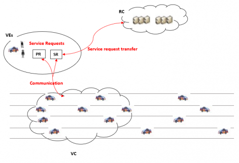
We consider a system of VCC as shown in Figure 1, in which moving vehicles constitute a dynamic VC. The cloud structure in the system is composed of two layers, remote cloud RC that consists of multiple powerful computing resources and vehicular cloud VC that constitutes some VEs. Each vehicle has a standard computing Resource Unit (RU) in the system. These units are managed and allocated via the VC. The capability of the VC to compute depends on the number of RUs in the VC.
Considering two categories of service requests:
Figure 1. Scheme of the proposed VCC system
Suppose there are M RUs available in the VC that vary with time because it depends on the arrival and the departure of vehicles.
Let $\left(N_{t}^{\lambda_{p}}, t>0\right),\left(N_{t}^{\lambda_{s}}, t>0\right), \text { and }\left(N_{t}^{\lambda_{v}}, t>0\right)$ three Poisson Processes with the mean rate of λp, λs, and λv respectively, where $N_{t}^{\lambda_{p}}, N_{t}^{\lambda_{s}}, \text { and } N_{t}^{\lambda_{v}}$, for each t>0, are the number of PRs arrivals, the number of SRs arrivals, and the number of arrival of vehicles, in the interval time (0,t] respectively.
Each arrival service request PR can be allocated with i RUs in the VC, where i∈{1,...,N}, N≤M and N is the maximum number of RUs that can allocate to a service request PR by the VC. The same if an arrival service request SR is accepted to assign to the VC.
The service rate of the PR and SR are denoted by μp and μs respectively. Then $\frac{1}{i \mu_{p}}$ is the service time of a request PR if i RUs are allocated and $\frac{1}{i \mu_{s}}$ for SR if it is accepted to assign to VC. Assume that $\lambda_{p}<M \mu_{p}$ to ensure that the system is accessible and stable for PRs. The number of RUs in the VC can not be larger than K. In addition, the departure of vehicle follows Poisson distribution with rate μv.
Furthermore, when all of the resources units RUs are full, since the system firstly keeps the RUs to the primary requests PRs, we must transfer SR’ s service which occupies the RUs to the RC.
The main objective is to maximize the expected long-term total reward by using the SMDP approach correctly allocating VCC system resources to PR and SR.
3.2 System states
We consider two types of service requests PR and SR.
We use S to denote the state set that can be represented by current requests, the usable resources in the VC and the event, i.e.,
S={s(t)/s(t)=<xs (t),xp (t),M,e>} (1)
where, $x_{s}(t)=\left[x_{s}^{1}(t), \ldots, x_{s}^{N}(t)\right]^{t}$, $x_{s}^{i}(t)$ is the number of SRs that have been allocated with i RUs i∈{1,...,N} at time t. Similarly, $x_{p}(t)=\left[x_{p}^{1}(t), \ldots, x_{p}^{N}(t)\right]^{t}$, $x_{p}^{i}(t)$ is the number of PRs that have been allocated with i RUs, M is the number of available RUs in the VC and e represents an event in the set as mentioned in Table 1.
$\mathcal{E}=\left\{A_{p}, A_{s}, A_{v}, D_{v}, D_{p}^{i}, D_{s}^{i}\right\}$ (2)
where,
Table 1. Summary of events
|
e |
Event |
|
$A_{p}$ |
PR arrival |
|
$A_{S}$ |
SR arrival |
|
$A_{v}$ |
arrival of vehicle |
|
$D_{v}$ |
departure of vehicle |
|
$D_{p}^{i}$ |
departure of a PR allocated with $i$ RUs |
|
$D_{S}^{i}$ |
departure of a SR allocated with $i$ RUs |
Therefrom $\sum_{i=1}^{N} i\left(x_{p}^{i}(t)+x_{s}^{i}(t)\right)$ is the number of occupied RUs in the VC which satisfies $\sum_{i=1}^{N} i\left(x_{p}^{i}(t)+x_{s}^{i}(t)\right) \leq M$.
3.3 Actions
When the system receives a request, it can choose an action as follows. If the SR request has been accepted with i RUs, the action denotesa(t)=(S,i).
Therefore, a(t)=(S,0) indicates that when a SR arrives and the VC is full, the VC will transfer it to the RC. Otherwise, if the accepted PR request with i RUs, it denotes as a(t)=(P,i) .
a(t)=-1 describes that no action is required except updating the number of RUs in the system when a vehicle arrives and leaves the system or a service request finish and exits the VCC system. The action space $\mathcal{A}(t)$ is summarized as follows:
$\mathcal{A}(t)= \begin{cases}-1 & , e \in\left\{A_{v}, D_{v}, D_{p}^{i}, D_{s}^{i}\right\} \\ (P, i) & , e=A_{p} \\ \{(S, i),(S, 0)\} & , e=A_{s} .\end{cases}$ (3)
3.4 Transition probability
Let τ(s(t),a(t)) be the expected service time between two continuous decision epoch and σ(s(t),a(t)) be the mean event rate for specific s(t) and a(t) which can be expressed by σ(s(t), $a(t))=\frac{1}{\tau(s(t), a(t))}$ with,
$\sigma(s(t), a(t))= \begin{cases}(M+1)\left(\lambda_{p}+\lambda_{s}\right)+\lambda_{v}+\mu_{v}+\sum_{j=1}^{N} j\left(x_{s}^{j}(t) \mu_{s}+x_{p}^{j}(t) \mu_{p}\right) & \text { if } e=A_{v}, a(t)=-1 \\ (M-1)\left(\lambda_{p}+\lambda_{s}\right)+\lambda_{v}+\mu_{v}+\sum_{j=1}^{N} j\left(x_{s}^{j}(t) \mu_{s}+x_{p}^{j}(t) \mu_{p}\right) & \text { if } e=D_{v}, a(t)=-1 \\ M\left(\lambda_{p}+\lambda_{s}\right)+\lambda_{v}+\mu_{v}+\sum_{j=1}^{N} j\left(x_{s}^{j}(t) \mu_{s}+x_{p}^{j}(t) \mu_{p}\right) & \text { if } e=A_{s}, a(t)=(S, 0) \\ M\left(\lambda_{p}+\lambda_{s}\right)+\lambda_{v}+\mu_{v}+\sum_{j=1}^{N} j\left(x_{s}^{j}(t) \mu_{s}+x_{p}^{j}(t) \mu_{p}\right)+i \mu_{s} & \text { if } e=A_{s}, a(t)=(S, i) \\ M\left(\lambda_{p}+\lambda_{s}\right)+\lambda_{v}+\mu_{v}+\sum_{j=1}^{N} j\left(x_{s}^{j}(t) \mu_{s}+x_{p}^{j}(t) \mu_{p}\right)+i \mu_{p} & \text { if } e=A_{p}, a(t)=(P, i) \\ M\left(\lambda_{p}+\lambda_{s}\right)+\lambda_{v}+\mu_{v}+\sum_{j=1}^{N} j\left(x_{s}^{j}(t) \mu_{s}+x_{p}^{j}(t) \mu_{p}\right)-i \mu_{s} & \text { if } e=D_{s}^{i}, a(t)=-1 \\ M\left(\lambda_{p}+\lambda_{s}\right)+\lambda_{v}+\mu_{v}+\sum_{j=1}^{N} j\left(x_{s}^{j}(t) \mu_{s}+x_{p}^{j}(t) \mu_{p}\right)-i \mu_{p} & \text { if } e=D_{p}^{i}, a(t)=-1 .\end{cases}$ (4)
μv is vehicle departure rate and (M(λp+λs )+λv) is the total arrived rate of requests and vehicles. Since λp and λs are the arrival rates for PR and SR request per vehicle respectively then M(λp+λs ) is the arrival rate of requests of the VCC system.
The rate at which requests leave the system is as described next. If a vehicle enters or departs the system then the total RUs are not modified. Thus $\sum_{j=1}^{N} j\left(x_{s}^{j}(t) \mu_{s}+x_{p}^{j}(t) \mu_{p}\right)$ is the departure rate of requests. If a PR arrives at the system, the departure rate is $\sum_{j=1}^{N} j\left(x_{s}^{j}(t) \mu_{s}+x_{p}^{j}(t) \mu_{p}\right)+i \mu_{p}$. If a SR arrives, the departure rate is given by $\sum_{j=1}^{N} j\left(x_{s}^{j}(t) \mu_{s}+x_{p}^{j}(t) \mu_{p}\right)+i \mu_{s}$.
When a PR is served and leaves the system, the departure rate of requests is computed as $\sum_{j=1}^{N} j\left(x_{s}^{j} \mu_{s}+x_{p}^{j}(t) \mu_{p}\right)-i \mu_{p}$. Thus, if a SR is completed the service, then the departure rate of requests is computed as $\sum_{j=1}^{N} j\left(x_{s}^{j}(t) \mu_{s}+x_{p}^{j}(t) \mu_{p}\right)-i \mu_{s}$.
Next, from the probability theory, σ(s(t),a(t)) is the denominator of the transition probability.
Let P(s'/s(t),a(t)) is the probability of transition from state s(t) to state s' under an action a(t). We formulate the model so that transitions which occur between decision epochs do not influence the decision. This transition probability can be calculated under different events (5)-(9):
• State s(t)=<xs (t),xp (t),M,Ap>.
$P\left(s^{\prime} / s(t), a(t)\right)=\left\{\begin{array}{lll}
\frac{\left(x_{p}^{i}(t)+1\right) i \mu_{p}}{\sigma(s(t), a(t))} & \text { if } s^{\prime}=\left\langle x_{s}(t), x_{p}(t)+e_{i}-e_{i}, M, D_{p}^{i}\right\rangle, & a(t)=(P, i) \\
\frac{x_{p}^{m}(t) m \mu_{p}}{\sigma(s(t), a(t))} & \text { if } s^{\prime}=\left\langle x_{s}(t), x_{p}(t)+e_{i}-e_{m}, M, D_{p}^{m}\right\rangle, & a(t)=(P, i) \\
\frac{x_{S}^{m}(t) m \mu_{s}}{\sigma(s(t), a(t))} & \text { if } s^{\prime}=\left\langle x_{s}(t)-e_{m}, x_{p}(t)+e_{i}, M, D_{s}^{m}\right\rangle, & a(t)=(P, i) \\
\frac{M \lambda_{s}}{\sigma(s(t), a(t))} & \text { if } s^{\prime}=\left\langle x_{s}(t), x_{p}(t)+e_{i}, M, A_{s}\right\rangle, & a(t)=(P, i) \\
\frac{M \lambda_{p}}{\sigma(s(t), a(t))} & \text { if } s^{\prime}=\left\langle x_{s}(t), x_{p}(t)+e_{i}, M, A_{p}\right\rangle, & a(t)=(P, i) \\
\frac{\lambda_{v}}{\sigma(s(t), a(t))} & \text { if } s^{\prime}=\left\langle x_{s}(t), x_{p}(t)+e_{i}, M, A_{v}\right\rangle, & a(t)=(P, i) \\
\frac{\mu_{v}}{\sigma(s(t), a(t))} & \text { if } s^{\prime}=\left\langle x_{s}(t), x_{p}(t)+e_{i}, M, D_{v}\right\rangle, & a(t)=(P, i)
\end{array}\right.$ (5)
where, a(t)=(P,i) , i∈{1,...,N}, m∈{1,...,N} and i≠m. Let $e_{i}$ is a vector of N components, where the i-th component is 1, others are 0. The same for the vector em.
• State s=<xs (t),xp (t),M,Av>.
$P\left(s^{\prime} / s(t), a(t)\right)=\left\{\begin{array}{lll}
\frac{x_{p}^{i}(t) i \mu_{p}}{\sigma(s(t), a(t))} & \text { if } s^{\prime}=\left\langle x_{s}(t), x_{p}(t), M+1, D_{p}^{i}\right\rangle, & a(t)=-1 \\
\frac{x_{S}^{i}(t) i \mu_{s}}{\sigma(s(t), a(t))} & \text { if } s^{\prime}=\left\langle x_{s}(t), x_{p}(t), M+1, D_{s}^{i}\right\rangle, & a(t)=-1 \\
\frac{(M+1) \lambda_{s}}{\sigma(s(t), a(t))} & \text { if } s^{\prime}=\left\langle x_{s}(t), x_{p}(t), M+1, A_{s}\right\rangle, & a(t)=-1 \\
\frac{(M+1) \lambda_{p}}{\sigma(s(t), a(t))} & \text { if } s^{\prime}=\left\langle x_{s}(t), x_{p}(t), M+1, A_{p}\right\rangle, & a(t)=-1 \\
\frac{\lambda_{v}}{\sigma(s(t), a(t))} & \text { if } s^{\prime}=\left\langle x_{s}(t), x_{p}(t), M+1, A_{v}\right\rangle, & a(t)=-1 \\
\frac{\mu_{v}}{\sigma(s(t), a(t))} & \text { if } s^{\prime}=\left\langle x_{s}(t), x_{p}(t), M+1, D_{v}\right\rangle, & a(t)=-1
\end{array}\right.$ (6)
• State $s(t)=<x_{s}(t), x_{p}(t), M, A_{s}>$.
$P\left(s^{\prime} / s(t), a(t)\right)=\left\{\begin{array}{lll}
\frac{x_{p}^{i}(t) i \mu_{p}}{\sigma(s(t), a(t))} & \text { if } s^{\prime}=\left\langle x_{s}(t), x_{p}(t)-e_{i}, M, D_{p}^{i}\right\rangle, & a(t)=(S, 0) \\
\frac{x_{s}^{i}(t) i \mu_{s}}{\sigma(s(t), a(t))} & \text { if } s^{\prime}=\left\langle x_{s}(t)-e_{i}, x_{p}(t), M, D_{s}^{i}\right\rangle, & a(t)=(S, 0) \\
\frac{M \lambda_{s}}{\sigma(s(t), a(t))} & \text { if } s^{\prime}=\left\langle x_{s}(t), x_{p}(t), M, A_{s}\right\rangle, & a(t)=(S, 0) \\
\frac{M \lambda_{p}}{\sigma(s(t), a(t))} & \text { if } s^{\prime}=\left\langle x_{s}, x_{p}(t), M, A_{p}\right\rangle, & a(t)=(S, 0) \\
\frac{\lambda_{v}}{\sigma(s(t), a(t))} & \text { if } s^{\prime}=\left\langle x_{s}(t), x_{p}(t), M, A_{v}\right\rangle, & a(t)=(S, 0) \\
\frac{\mu_{v}}{\sigma(s(t), a(t))} & \text { if } s^{\prime}=\left\langle x_{s}(t), x_{p}(t), M, D_{v}\right\rangle, & a(t)=(S, 0) \\
\frac{\left(x_{S}^{i}(t)+1\right) i \mu_{s}}{\sigma(s(t), a(t))} & \text { if } s^{\prime}=\left\langle x_{s}(t), x_{p}(t), M, D_{s}^{i}\right\rangle, & a(t)=(S, i) \\
\frac{x_{s}^{m}(t) m \mu_{s}}{\sigma(s(t), a(t))} & \text { if } s^{\prime}=\left\langle x_{s}(t)+e_{i}-e_{m}, x_{p}(t), M, D_{s}^{m}\right\rangle, & a(t)=(S, i) \\
\frac{x_{p}^{m}(t) m \mu_{p}}{\sigma(s(t), a(t))} & \text { if } s^{\prime}=\left\langle x_{s}(t)+e_{i}, x_{p}(t)-e_{m}, M, D_{p}^{m}\right\rangle, & a(t)=(S, i) \\
\frac{M \lambda_{s}}{\sigma(s(t), a(t))} & \text { if } s^{\prime}=\left\langle x_{s}(t)+e_{i}, x_{p}(t), M, A_{s}\right\rangle, & a(t)=(S, i) \\
\frac{M \lambda_{p}}{\sigma(s(t), a(t))} & \text { if } s^{\prime}=\left\langle x_{s}(t), x_{p}(t)+e_{i}, M, A_{p}\right\rangle, & a(t)=(S, i) \\
\frac{\lambda_{v}}{\sigma(s(t), a(t))} & \text { if } s^{\prime}=\left\langle x_{s}(t), x_{p}(t), M, A_{v}\right\rangle, & a(t)=(S, i) \\
\frac{\mu_{v}}{\sigma(s(t), a(t))} & \text { if } s^{\prime}=\left\langle x_{s}(t), x_{p}(t), M, D_{v}\right\rangle, & a(t)=(S, i) \\
&
\end{array}\right.$ (7)
where, i∈{1,...,N} , m∈{1,...,N} and i≠m.
• State $s=<x_{s}(t), x_{p}(t), M, D_{v}>$.
$P\left(s^{\prime} / s(t), a(t)\right)=\left\{\begin{array}{lll}
\frac{x_{p}^{i}(t) i \mu_{p}}{\sigma(s(t), a(t))} & \text { if } s^{\prime}=\left\langle x_{s}(t), x_{p}(t), M-1, D_{p}^{i}\right\rangle, & a(t)=-1 \\
\frac{x_{s}^{i} i \mu_{s}}{\sigma(s(t), a(t))} & \text { if } s^{\prime}=\left\langle x_{s}(t), x_{p}(t), M-1, D_{s}^{i}\right\rangle, & a(t)=-1 \\
\frac{(M-1) \lambda_{s}}{\sigma(s(t), a(t))} & \text { if } s^{\prime}=\left\langle x_{s}(t), x_{p}(t), M-1, A_{s}\right\rangle, & a(t)=-1 \\
\frac{(M-1) \lambda_{p}}{\sigma(s(t), a(t))} & \text { if } s^{\prime}=\left\langle x_{s}(t), x_{p}(t), M-1, A_{p}\right\rangle, & a(t)=-1 \\
\frac{\lambda_{v}}{\sigma(s(t), a(t))} & \text { if } s^{\prime}=\left\langle x_{s}(t), x_{p}(t), M-1, A_{v}\right\rangle, & a(t)=-1 \\
\frac{\mu_{v}}{\sigma(s(t), a(t))} & \text { if } s^{\prime}=\left\langle x_{s}(t), x_{p}(t), M-1, D_{v}\right\rangle, & a(t)=-1 \\
&
\end{array}\right.$ (8)
• State $s=<x_{s}(t), x_{p}(t), M, e>\text { where } e \in\left\{D_{p}^{i}, D_{s}^{i}\right\}$.
$P\left(s^{\prime} / s(t), a(t)\right)=\left\{\begin{array}{lll}
\frac{x_{p}^{i}(t) i \mu_{p}}{\sigma(s(t), a(t))} & \text { if } s^{\prime}=\left\langle x_{s}(t), x_{p}(t)-e_{i}, M, D_{p}^{i}\right\rangle, & a(t)=-1 \\
\frac{x_{S}^{i}(t) i \mu_{s}}{\sigma(s(t), a(t))} & \text { if } s^{\prime}=\left\langle x_{s}(t)-e_{i}, x_{p}(t), M, D_{s}^{i}\right\rangle, & a(t)=-1 \\
\frac{M \lambda_{s}}{\sigma(s(t), a(t))} & \text { if } s^{\prime}=\left\langle x_{s}(t), x_{p}(t), M, A_{s}\right\rangle, & a(t)=-1 \\
\frac{M \lambda_{p}}{\sigma(s(t), a(t))} & \text { if } s^{\prime}=\left\langle x_{s}(t), x_{p}(t), M, A_{p}\right\rangle, & a(t)=-1 \\
\frac{\lambda_{v}}{\sigma(s(t), a(t))} & \text { if } s^{\prime}=\left\langle x_{s}(t), x_{p}(t), M, A_{v}\right\rangle, & a(t)=-1 \\
\frac{\mu_{v}}{\sigma(s(t), a(t))} & \text { if } s^{\prime}=\left\langle x_{s}(t), x_{p}(t), M, D_{v}\right\rangle, & a(t)=-1
\end{array}\right.$ (9)
3.5 Reward model
Let r(s(t),a(t)) denote the system reward under the state s(t) and the action a(t) then we have:
r(s,a)=k(s(t),a(t))-g(s(t),a(t)) (10)
where, k(s(t),a(t)) is the instant income of the system under the state s(t) and the action a(t) in the case that event e occurs and g(s(t),a(t)) is the expected system cost.
Through the priority of service requests, we obtain six cases for k(s(t),a(t)) as follows:
$k(s(t), a(t))=\left\{\begin{array}{c}
\omega_{e} \beta_{e}\left(E_{0}-P \delta_{1}\right)+\omega_{d} \beta_{d}\left(D_{0}-\frac{1}{i \mu_{s}}-\delta_{1}\right)-\gamma \delta_{1} \quad a(t)=-1 \\
0 \quad \text { if } e \in\left\{D_{p}, D_{s}, A_{v}\right\}, a(t)=-1 \\
0 \quad \text { if } e=D_{v}, a(t)=-1, \sum_{i=1}^{N} i\left(x_{p}^{i}(t)+x_{s}^{i}(t)\right)<M \\
-\xi \quad \text { if } e=D_{v}, a(t)=-1, \sum_{i=1}^{N} i\left(x_{p}^{i}(t)+x_{s}^{i}(t)\right)=M \\
\omega_{e} \beta_{e}\left(E_{0}-P \delta_{1}\right)+\omega_{d} \beta_{d}\left(D_{0}-\delta_{1}-\delta_{2}\right)-\gamma\left(\delta_{1}+\delta_{2}\right) \quad \text { if } e=A_{s}, a(t)=(S, 0) \\
\omega_{e} \beta_{e}\left(E_{0}-P \delta_{1}\right)+\omega_{d} \beta_{d}\left(D_{0}-\frac{1}{i \mu_{p}}-\delta_{1}\right)-\gamma\left(\delta_{1}+\delta_{2}\right)-\delta_{0} \quad \text { if } e=A_{p}, a(t)=(P, i)
\end{array}\right.$ (11)
where, $\left(E_{0}-P \delta_{1}\right) \text { and }\left(D_{0}-\frac{1}{i \mu_{s}}-\delta_{1}\right)$ are respectively the energy and the time saved during the processing task in the VC. Pδ1 is the workload of transferring the task to VC and receiving the feedback from it. γδ1 is the transfer expense.
The VCC system generates nothing when a service leaves the system or a vehicle arrives.
The price ξ occurred when all RUs used and a vehicle departs the VC.
The SR request may be transferred to the RC if the available resources in the VC are not sufficient. γδ2 is the transfer cost of the job to the RC and the feedback from it. Without considering the processing time, the cost of transfer expense is given by $\left[\omega_{e} \beta_{e}\left(E_{0}-P \delta_{1}\right)+\omega_{d} \beta_{d}\left(D_{0}-\delta_{1}-\delta_{2}\right)\right]$ due to the powerful computing capability of the RC.
The list of important used parameters is given in Table 2.
Table 2. List of important parameters
|
$\omega_{e} / \omega_{d}$ |
The weights of power/time where $\omega_{e}+\omega_{d}=1$ |
|
$\beta_{e} / \beta_{d}$ |
Price of per energy/delay saving |
|
$E_{0}$ |
The workload occurs by executing the request at VE |
|
$D_{0}$ |
The time occurs by executing the request at VE |
|
$P$ |
Transmission power of Ves |
|
$\gamma$ |
Cost per transmit time |
|
$\delta_{1}$ |
Delay of transfer from VE to VC |
|
$\delta_{2}$ |
Delay of transfer from VC to RC |
|
$\delta_{0}$ |
Cost of sending to a RU. |
|
$\xi$ |
Vehicle control via the VCC system |
Next, we define the expected system cost g(s(t),a(t)) as follows:
g(s(t),a(t))=c(s(t),a(t))τ(s(t),a(t)), (12)
where, τ(s(t),a(t)) is the expected service time, and c(s(t),a(t)) is the number of the RUs that have been allocated, i.e.,
$c(s(t), a(t))=\sum_{i=1}^{N} i\left(x_{p}^{i}(t)+x_{s}^{i}(t)\right).$ (13)
Due to the fact that vehicle arrivals and departures and service requests are distributed according to the Poisson distribution, there is an exponential distribution of time taken from decision time to decision time.
$F(t / s, a)=1-e^{\sigma(s(t), a(t)) t}\quad \text { for } t>0.$ (14)
Moreover, according to the discounted reward model found in Ref. [14], the expected discounted reward is given by:
$\begin{aligned}
r(s(t), a(t))=k &(s(t), a(t)) \\
&-c(s(t), a(t)) E_{s(t)}^{a(t)}\left\{\int_{0}^{\tau} e^{-\alpha t} d t\right\} \\
&=k(s(t), a(t)) \\
&-c(s(t), a(t)) E_{s(t)}^{a(t)}\left\{\frac{1-e^{-\alpha \tau}}{\alpha}\right\} \\
&=k(s(t), a(t)) \\
&-\frac{c(s(t), a(t))}{\alpha+\sigma(s(t), a(t))}
\end{aligned}$ (15)
where, α is a discount factor.
3.6 Solution
According to Bellman's equation, the maximum reward is obtained as below,
$\begin{gathered}
v(s(t))=\max _{a(t) \in \mathcal{A}} \\
\left\{r\left(s(t), a(t)+\lambda \sum_{s \in \mathcal{S}} p\left(s^{\prime} / s(t), a(t)\right) v\left(s^{\prime}\right)\right\},\right.
\end{gathered}$ (16)
where, $\lambda=\frac{\sigma(s(t), a(t))}{\alpha+\sigma(s(t), a(t))}$. In order to achieve the unified expected system reward, we define the parameter $y=K\left(\lambda_{p}+\lambda_{s}\right)+\lambda_{v}+\mu_{v}+N K\left(\mu_{p}+\mu_{s}\right)$.
Then, the normalized transition probability is given as follows:
$\begin{aligned}
&\hat{p}\left(s^{\prime} / s, a\right) \\
&= \begin{cases}\frac{p\left(s^{\prime} / s, a\right) \sigma(s, a)}{y} & s^{\prime} \neq s \\
1-\frac{\left[1-p\left(s^{\prime} / s, a\right)\right] \sigma(s, a)}{y}, & s^{\prime}=s .\end{cases}
\end{aligned}$ (17)
The normalized reward function (10) is,
$\hat{r}(s, a)=r(s, a) \frac{\sigma(s, a)+\alpha}{y+\alpha}.$ (18)
Accordingly, Eq. (16) can be expressed as:
$\hat{v}(s)=\max _{a \in \mathcal{A}}\left\{\hat{r}(s, a)+\hat{\lambda} \sum_{s^{\prime} \in \mathcal{S}} \hat{p}\left(s^{\prime} / s, a\right) \hat{v}\left(s^{\prime}\right)\right\}$ (19)
where, $\hat{\lambda}=\frac{y}{y+\alpha}$ .
Then, we propose the value iteration algorithm to solve the optimization problem given by Eq. (19).
Algorithm 1
Step 1: $\text { S } \hat{v}(s(t)) \text { et }$ for each state s(t). Specify ϵ>0, and set k=0.
Step 2: For each state s(t), compute $\hat{v}^{k+1}(s(t))$ by:
$\begin{gathered}
\hat{v}^{k+1}(s)=\max _{a(t) \in \mathcal{A}} \\
\left\{\hat{r}(s(t), a(t))+\hat{\lambda} \sum_{s^{\prime} \in \mathcal{S}} \hat{p}\left(\frac{s^{\prime}}{s(t)}, a(t)\right) \hat{v}^{k}\left(s^{\prime}\right)\right\}
\end{gathered}$
Step 3: If $\left\|\hat{v}^{k+1}-\hat{v}^{k}\right\|<\epsilon(1-\hat{\lambda}) / 2 \hat{\lambda}$, go to Step 4. Else k=k+1, return to Step 2.
Step 4: For each $s \in \mathcal{S}$, compute the stationary optimal policy and stop.
$\begin{gathered}
d_{\epsilon}^{*} \in \operatorname{argmax}_{a(t) \in \mathcal{A}} \\
{\left[\hat{r}(s(t), a(t))+\hat{\lambda} \sum_{s^{\prime} \in \mathcal{S}} \hat{p}\left(s^{\prime} / s(t), a(t)\right) \hat{v}^{k+1}\left(s^{\prime}\right)\right]}
\end{gathered}$
The norm function is defined as $\|\hat{v}\|=\max |\hat{v}(s(t))|$ for s(t)∈S.
Here, we evaluate the efficiency of the model. We provide the numerical results under different scenario. The main parameters are given in Table 3.
Table 3. List of parameter values
|
Parameter |
Value |
Parameter |
Value |
Parameter |
Value |
|
$\lambda_{v}$ |
6 |
$\mu_{p}$ |
7 |
$\mu_{s}$ |
11 |
|
$\mu_{v}$ |
11 |
$\alpha$ |
0.1 |
$\omega_{e}$ |
0.5 |
|
$\omega_{d}$ |
0.5 |
$\beta_{e}$ |
2 |
$\beta_{d}$ |
2 |
|
$E_{0}$ |
20 |
$D_{0}$ |
30 |
$\gamma$ |
2 |
|
$\delta_{0}$ |
1 |
$\delta_{1}$ |
2 |
$\delta_{2}$ |
5 |
|
$\xi$ |
18 |
$K$ |
13 |
|
|
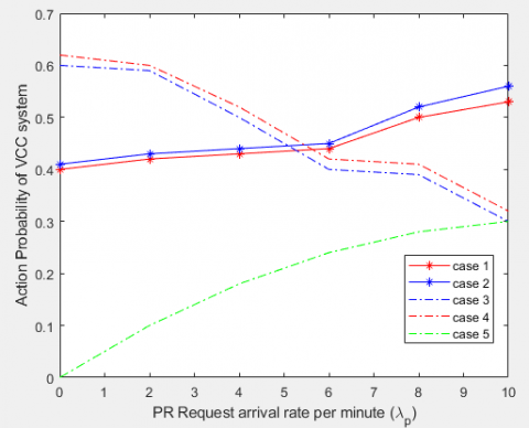
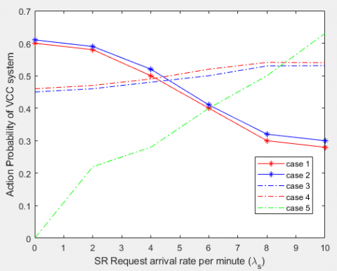
Let N=2 be the number of RUs reserved for a service request that is to say a service can be assigned 1 or 2 RUs.
Case 1 and Case 2 (respectively, Case 3 and Case 4) represent that the PR request allocates to the VC with 1 and 2 RUs (respectively, the SR request to the VC with 1 and 2 RUs). Besides, Case 5 is that the VCC system transfers the SR request to RC.
Figure 2. The action probabilities of Primary service requests
Figure 3. The action probabilities of Secondary service requests
Figures 2 and 3 present the action probability of the service requests under two parameters $\lambda_{p} \text { and } \lambda_{s}$. As Figure 2 illustrates, under conditions of low SR arrival rate, the probability of allocating SR requests to the VC (Case 3 and Case 4) is more than the probability of transferring to the RC (Case 5).
Also, when allocating a request to the VC, the VCC system tends to assign a maximum number of RUs to achieve the highest possible system rewards by considering the priority of the PR request. With the increase of the vehicle arrival rate, especially when the system accepts more PR arrival service requests, the probability of case 1 and case 2 starts to decrease. On the other hand, the probability of case 3 and case 4 increases and this depends on the advantage of PR arrival in our model system, and we notice that the rate of decrease in the probability of case 1 and case 2 makes sense because in our system, even if the PR arrival rate increases, SR arrival requests are also accepted but with low probability.
Furthermore, in Figure 3, while the probabilities of Case 1 and Case 2 begin to decrease and those of Case 3 and Case 4 increase slightly then the probability of Case 5 becomes larger.
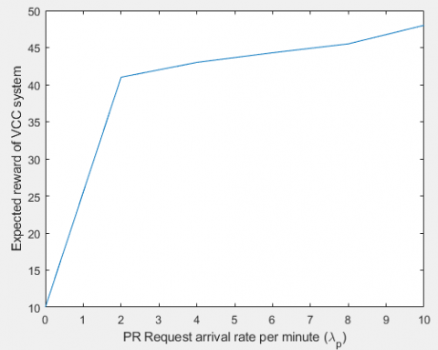
Next, we analyze the performance of VCC system. Figure 4 shows that the expected reward of system increase with the increases of the arrival rate of primary service requests.
Figure 4. System reward of primary service requests
Through this article, two types of service requests are considered with different priority in the Vehicular Cloud Computing (VCC) system based on the Semi-Markov infinite horizon decision process SMDP. We have used an iterative algorithm in order to maximize the reward model of the VCC system where primary service requests are given a higher priority to access the system in our policy. Numerical analysis showed that the used strategy to affect the resource units to the requests and the arrival rates of requests have impact on the system performance.
The study of this system in a dynamic manner is a perspective to extend the results obtained in this paper.
In our future work, we expect to consider the non-uniformity of service demands and how they affect on resource allocation. In addition, it would be valuable to explore the vehicle direction and speed.
[1] Zhang, T., De Grande, R.E., Boukerche, A. (2015). Vehicular cloud: Stochastic analysis of computing resources in a road segment. In Proceedings of the 12th ACM Symposium on Performance Evaluation of Wireless Ad Hoc, Sensor, & Ubiquitous Networks, pp. 9-16. https://doi.org/10.1145/2810379.2810383
[2] Baguena, M., Calafate, C.T., Cano, J.C., Manzoni, P. (2015). An adaptive anycasting solution for crowd sensing in vehicular environments. IEEE Transactions on Industrial Electronics, 62(12): 7911-7919. https://doi.org/10.1109/TIE.2015.2447505
[3] Hussain, R., Son, J., Eun, H., Kim, S., Oh, H. (2012). Rethinking vehicular communications: Merging VANET with cloud computing. In 4th IEEE International Conference on Cloud Computing Technology and Science Proceedings, pp. 606-609. https://doi.org/10.1109/CloudCom.2012.6427481
[4] Liu, N., Liu, M., Lou, W., Chen, G., Cao, J. (2011). PVA in VANETs: Stopped cars are not silent. In 2011 Proceedings IEEE INFOCOM, pp. 431-435. https://doi.org/10.1109/INFCOM.2011.5935198
[5] Gu, L., Zeng, D., Guo, S., Ye, B. (2013). Leverage parking cars in a two-tier data center. In 2013 IEEE Wireless Communications and Networking Conference (WCNC), pp. 4665-4670. https://doi.org/10.1109/WCNC.2013.6555330
[6] Eckhoff, D., Sommer, C., German, R., Dressler, F. (2011). Cooperative awareness at low vehicle densities: How parked cars can help see through buildings. In 2011 IEEE Global Telecommunications Conference-GLOBECOM, pp. 1-6. https://doi.org/10.1109/GLOCOM.2011.6134402
[7] Goumidi, H., Aliouat, Z., Harous, S. (2020). Vehicular cloud computing security: A survey. Arabian Journal for Science and Engineering, 45(4): 2473-2499. https://doi.org/10.1007/s13369-019-04094-0
[8] Shah, S.H.H., Noor, S., Lei, S., Butt, A.S., Ali, M. (2021). Role of privacy/safety risk and trust on the development of prosumption and value co-creation under the sharing economy: A moderated mediation model. Information Technology for Development, 27(4): 718-735. https://doi.org/10.1080/02681102.2021.1877604
[9] Mistareehi, H., Islam, T., Manivannan, D. (2021). A secure and distributed architecture for vehicular cloud. Internet of Things, 13: 100355. https://doi.org/10.1016/j.iot.2020.100355
[10] Meng, H., Zheng, K., Chatzimisios, P., Zhao, H., Ma, L. (2015). A utility-based resource allocation scheme in cloud-assisted vehicular network architecture. In 2015 IEEE International Conference on Communication Workshop (ICCW), pp. 1833-1838. https://doi.org/10.1109/ICCW.2015.7247447
[11] Zheng, K., Meng, H., Chatzimisios, P., Lei, L., Shen, X. (2015). An SMDP-based resource allocation in vehicular cloud computing systems. IEEE Transactions on Industrial Electronics, 62(12): 7920-7928. https://doi.org/10.1109/TIE.2015.2482119
[12] Lin, C.C., Deng, D.J., Yao, C.C. (2017). Resource allocation in vehicular cloud computing systems with heterogeneous vehicles and roadside units. IEEE Internet of Things Journal, 5(5): 3692-3700. https://doi.org/10.1109/JIOT.2017.2690961
[13] Behbehani, F.S., Elgorashi, T., Elmirghani, J.M. (2021). Power Minimization in Vehicular Cloud Architecture. arXiv preprint arXiv:2102.09011.
[14] Ouammou, A., Hanini, M., Tahar, A.B., El Kafhali, S. (2019). Analysis of a M/M/k system with exponential setup times and reserves servers. In Proceedings of the 4th International Conference on Big Data and Internet of Things, 1-5. https://doi.org/10.1145/3372938.3372996
[15] Ouammou, A., Tahar, A.B., Hanini, M., El Kafhali, S. (2018). Modeling and analysis of quality of service and energy consumption in cloud environment. International Journal of Computer Information Systems and Industrial Management Applications, 10: 98-106.
[16] Ouammou, A., Zaaloul, A., Hanini, M., Bentahar, A. Modeling decision making to control the allocation of virtual machines in a cloud computing system with reserve machines. IAENG International Journal of Computer Science, 48(2): 285-293.
[17] Hanini, M., Kafhali, S.E., Salah, K. (2019). Dynamic VM allocation and traffic control to manage QoS and energy consumption in cloud computing environment. International Journal of Computer Applications in Technology, 60(4): 307-316. https://doi.org/10.1504/IJCAT.2019.101168