Iman I. Gorial
© 2021 IIETA. This article is published by IIETA and is licensed under the CC BY 4.0 license (http://creativecommons.org/licenses/by/4.0/).
OPEN ACCESS
The purpose of this work is to use a new numerical technique for solving the two-sided multi-dimensional variable order fractional mobile/immobile diffusion equation with non-local conditions (TSMDVOF-MIDENLCs) model using the variable time fractional derivative of Caputo, as well as an initial boundary value problem of modified treatment. We used the fractional variational iteration method (FVIM) to mix initial and boundary conditions, resulting in for each iteration, a new initial solution. Convergence, sufficient conditions (SC) for system convergence, and error estimation are discussed. Some examples are given to illustrate the applicability of the novel suggested method, demonstrating that the numerical solution matches the exact solution and that the error is zero. Furthermore, this algorithm is easy and inexpensive to implement, and it demonstrates efficiency and accuracy.
Caputo fractional derivatives, fractional mobile/immobile diffusion model, non-local condition, two-sided multi-dimensional, fractional variational iteration method
The Fractional calculus is the generalization of the ordinary calculus which examines the integration and derivatives of the real or complex. Numerical methods have been used to solve functional equations that contain fractional derivatives, such as [1-7].
Thus, the theory and applications of partial calculus were rapidly developed. Fractional partial differential equations (FDEs) have been the focus of attention in recent decades as a possible representation for explaining anomalous diffusion and relaxation phenomena seen in a wide range of science and engineering fields [8-11], with applications in porous media fluid transport, plasma diffusion, liquid surface diffusion, surface production, and two-dimensional rotational flow. Also put a many of numerical methods for solving PDEs [12-18].
Zhang et al. [19] suggested an implicit numerical method with for solution variable fractional mobile-immobile advection-dispersion model subject to the Dirichlet condition, stability, and convergence.
Abdelkawy et al. [20] use numerical approach to solve the mobile / immobile advection-dispersion fractional time variable. Cheng et al. [21] determine the Caputo derivative order and the coefficient of diffusion. In addition, numerical treatment based upon finite difference methods for FDEs was presented [22-24]. While Finite element methods were introduced to obtain the numerical solutions of FDEs [25-27].
In other papers different variable fractional operator definitions for solving variable FDEs were discussed [28-34].
Additionally, the most developed methods today are finite difference methods for the numerical approximation of variable-order FDEs [35-38].
In this work, we aim to solution TSMDVOF-MIDENLCs model. The rest of this paper is arranged as follows. In section 2, mathematical aspects. In section 3, mobile/immobile diffusion equation with non-local conditions (MIDENLCs) model. In section 4, proposed method and its convergence. In section 5, test problems. Finally, we present conclusion about solution TSMDVOF-MIDENLCs in section 6.
2.1 Definition 1 Coimbra [31]
Order Caputo fractional derivative operator defined as form follows:
$D^{\propto(\sigma, \zeta)} f(\sigma)=\frac{1}{\Gamma(m-\alpha(\sigma, \zeta))} \int_{0}^{\sigma} \frac{f^{(m)}(\zeta)}{(\sigma-\zeta)^{\alpha(\sigma, \zeta)-m+1}} d \zeta$.
where, $\mathfrak{m}-1<\alpha(\sigma)<\mathfrak{m}, \mathfrak{m} \in N, \sigma>0$.
Caputo's derivative of the variable order, we have:
$D_{L_{+}}^{\alpha(\sigma)}(\sigma-L)^{n}=\frac{\Gamma(n+1)}{\Gamma(n+1-\alpha(\sigma))}(\sigma-L)^{n-\alpha(\sigma)}$,
and
$D_{R-}^{\alpha(\sigma)}(R-\sigma)^{n}=\frac{\Gamma(n+1)}{\Gamma(n+1-\alpha(w))}(R-\sigma)^{n-\alpha(\sigma)}$.
2.2 Definition 2 Coimbra [31]
If $\exists$ a real no. $C_{\vartheta}, \vartheta \in R$ is called in space where, $k(x), x>$ 0 a real function. $b(>\vartheta)$, s.t $k(x)=x^{b} k_{1}(x), k_{1} \in$ $C[0, \infty] .$ If $y \leq \vartheta$ then $C_{\vartheta} \subset C_{y}$.
2.3 Definition 3 Coimbra [31]
If $k^{(m)} \in \mathrm{C}_{\vartheta}$ then $\mathrm{C}_{\theta}^{m}, m \in N \cup\{0\}$ it is called in space where, $k(x), x>0$ a real function.
In this section, we present the TSMDVOF-MIDENLCs model:
$\beta_{1} D_{\zeta} \Omega\left(\sigma_{1}, \sigma_{2}, \ldots, \sigma_{n}, \zeta\right)$
$+\beta_{2} D_{+\zeta}^{\gamma\left(\sigma_{1}, \sigma_{2}, \ldots, \sigma_{n}, \zeta\right)} \Omega\left(\sigma_{1}, \sigma_{2}, \ldots, \sigma_{n}, \zeta\right)$
$\quad+\beta_{3} D_{-\zeta}^{\gamma\left(\sigma_{1}, \sigma_{2}, \ldots, \sigma_{n}, \zeta\right)} \Omega\left(\sigma_{1}, \sigma_{2}, \ldots, \sigma_{n}, \zeta\right)$
$\quad+\beta_{4} \sum_{i=1}^{n} D_{\sigma_{i}} \Omega\left(\sigma_{1}, \sigma_{2}, \ldots, \sigma_{n}, \zeta\right)$
$\quad-\beta_{5} \sum_{i=1}^{n} D_{\sigma_{i}}^{2} \Omega\left(\sigma_{1}, \sigma_{2}, \ldots, \sigma_{n}, \zeta\right)$
$=Q\left(\sigma_{1}, \sigma_{2}, \ldots, \sigma_{n}, \zeta\right), i$
$=1,2, \ldots, n .$ (1)
the initial condition (IC):
$\Omega\left(\sigma_{1}, \sigma_{2}, \ldots, \sigma_{n}, 0\right)=f\left(\sigma_{1}, \sigma_{2}, \ldots, \sigma_{n}\right), \quad 0 \leq \sigma_{i} \leq 1$ (2)
and the non-local boundary conditions (N-LBCs):
$\Omega\left(0, \sigma_{2}, \ldots, \sigma_{n}, \zeta\right)$
$=\int_{0}^{1} \varphi\left(\sigma_{1}, \sigma_{2}, \ldots, \sigma_{n}, \zeta\right) \Omega\left(\sigma_{1}, \sigma_{2}, \ldots, \sigma_{n}, \zeta\right) d \sigma_{1}$
$+L_{1}\left(\sigma_{1}, \sigma_{2}, \ldots, \sigma_{n}, \zeta\right)$,
$\Omega\left(\sigma_{1}, 0, \ldots, \sigma_{n}, \zeta\right)=\int_{0}^{1} \varphi\left(\sigma_{1}, \sigma_{2}, \ldots, \sigma_{n}, \zeta\right)$
$\Omega\left(\sigma_{1}, \sigma_{2}, \ldots, \sigma_{n}, \zeta\right) d \sigma_{2}+L_{2}\left(\sigma_{1}, \sigma_{2}, \ldots, \sigma_{n}, \zeta\right)$
$\vdots$
$\Omega\left(\sigma_{1}, \sigma_{2}, \ldots, 0, \zeta\right)$ $=\int_{0}^{1} \varphi\left(\sigma_{1}, \sigma_{2}, \ldots, \sigma_{n}, \zeta\right) \Omega\left(\sigma_{1}, \sigma_{2}, \ldots, \sigma_{n}, \zeta\right) d \sigma_{n}$
$+L_{n}\left(\sigma_{1}, \sigma_{2}, \ldots, \sigma_{n}, \zeta\right)$, $\Omega\left(1, \sigma_{2}, \ldots, \sigma_{n}, \zeta\right)$
$=\int_{0}^{1} \varphi\left(\sigma_{1}, \sigma_{2}, \ldots, \sigma_{n}, \zeta\right) \Omega\left(\sigma_{1}, \sigma_{2}, \ldots, \sigma_{n}, \zeta\right) d \sigma_{1}$
$+\quad M_{1}\left(\sigma_{1}, \sigma_{2}, \ldots, \sigma_{n}, \zeta\right)$ $\Omega\left(\sigma_{1}, 1, \ldots, \sigma_{n}, \zeta\right)$
$=\int_{0}^{1} \varphi\left(\sigma_{1}, \sigma_{2}, \ldots, \sigma_{n}, \zeta\right) \Omega\left(\sigma_{1}, \sigma_{2}, \ldots, \sigma_{n}, \zeta\right) d \sigma_{2}$$+M_{2}\left(\sigma_{1}, \sigma_{2}, \ldots, \sigma_{n}, \zeta\right)$,
$\vdots$
$\Omega\left(\sigma_{1}, \sigma_{2}, \ldots, 1, \zeta\right)$
$=\int_{0}^{1} \varphi\left(\sigma_{1}, \sigma_{2}, \ldots, \sigma_{n}, \zeta\right) \Omega\left(\sigma_{1}, \sigma_{2}, \ldots, \sigma_{n}, \zeta\right) d \sigma_{n}$
$+M_{n}\left(\sigma_{1}, \sigma_{2}, \ldots, \sigma_{n}, \zeta\right)$ (3)
where, $\beta_{1}, \beta_{2}, \beta_{3} \geq 0, \beta_{4}, \beta_{5}>0,0<\gamma \leq \gamma(\sigma, \zeta) \leq \bar{\gamma} \leq 1$, and $Q, f, L_{1}, L_{2}, \ldots, L_{n}$, and $M_{1}, M_{2}, \ldots, M_{n}$ are known functions, and $D^{\gamma\left(\sigma_{1}, \sigma_{2}, \ldots, \sigma_{n}, \zeta\right)}$ in our problem we define in terms of Caputo variable order fractional derivatives.
In this work, we used a new technique to calculate the zeroth approximation $\Omega_{0}^{*}$ by mixed initial conditions with boundary conditions at every iteration for get a new initial solution $\Omega_{0}^{*}$ by as follows:
(1) the initial solution can be written as:
Let
$\Omega\left(\sigma_{1}, \sigma_{2}, \ldots, \sigma_{n}, 0\right)=f_{0}\left(\sigma_{1}, \sigma_{2}, \ldots, \sigma_{n}\right), D_{\zeta} \Omega\left(\sigma_{1}, \sigma_{2}, \ldots, \sigma_{n}, 0\right)=f_{1}\left(\sigma_{1}, \sigma_{2}, \ldots, \sigma_{n}\right)$. (4)
Then,
$\begin{aligned} \Omega_{0}\left(\sigma_{1}, \sigma_{2}, \ldots, \sigma_{n},\right.&\zeta) =f_{0}\left(\sigma_{1}, \sigma_{2}, \ldots, \sigma_{n}\right) +\zeta f_{1}\left(\sigma_{1}, \sigma_{2}, \ldots, \sigma_{n}\right) \end{aligned}$, (5)
(2) We create a new successive initial solution $\Omega_{0}^{*}$ by applying a new technique at each iteration:
As,
$\Omega\left(0, \sigma_{2}, \ldots, \sigma_{n}, \zeta\right)=$
$\int_{0}^{1} \varphi\left(\sigma_{1}, \sigma_{2}, \ldots, \sigma_{n}, \zeta\right) \Omega\left(\sigma_{1}, \sigma_{2}, \ldots, \sigma_{n}, \zeta\right) d \sigma_{1}+$
$L_{1}\left(\sigma_{1}, \sigma_{2}, \ldots, \sigma_{n}, \zeta\right)$,
$\vdots$
$\Omega\left(\sigma_{1}, \sigma_{2}, \ldots, 0, \zeta\right)$ $=\int_{0}^{1} \varphi\left(\sigma_{1}, \sigma_{2}, \ldots, \sigma_{n}, \zeta\right) \Omega\left(\sigma_{1}, \sigma_{2}, \ldots, \sigma_{n}, \zeta\right) d \sigma_{n}$
$+L_{n}\left(\sigma_{1}, \sigma_{2}, \ldots, \sigma_{n}, \zeta\right)$,
$\Omega\left(1, \sigma_{2}, \ldots, \sigma_{n}, \zeta\right)$
$=\begin{gathered}\int_{0}^{1} \varphi\left(\sigma_{1}, \sigma_{2}, \ldots, \sigma_{n}, \rho\right) \Omega\left(\sigma_{1}, \sigma_{2}, \ldots, \sigma_{n}, \zeta\right) d \sigma_{1} \\ M_{1}\left(\sigma_{1}, \sigma_{2}, \ldots, \sigma_{n}, \zeta\right), \\ \vdots\end{gathered}$
$\Omega\left(\sigma_{1}, \sigma_{2}, \ldots, 1, \zeta\right)$
$=\int_{0}^{1} \varphi\left(\sigma_{1}, \sigma_{2}, \ldots, \sigma_{n}, \zeta\right) \Omega\left(\sigma_{1}, \sigma_{2}, \ldots, \sigma_{n}, \zeta\right) d \sigma_{n}$
$+M_{n}\left(\sigma_{1}, \sigma_{2}, \ldots, \sigma_{n}, \zeta\right) .$ (6)
Then,
$\begin{aligned} \Omega_{n}^{*}\left(\sigma_{1}, \sigma_{2}, \ldots, \sigma_{n}, \zeta\right) = \Omega_{n}\left(\sigma_{1}, \sigma_{2}, \ldots, \sigma_{n}, \zeta\right)+(1\left.-\sigma_{1}^{2}\right) \\\left[\int_{0}^{1} \varphi\left(\sigma_{1}, \sigma_{2}, \ldots,\right.\right.& \left.\sigma_{n}, \zeta\right) \Omega\left(\sigma_{1}, \sigma_{2}, \ldots, \sigma_{n}, \zeta\right) d \sigma_{1} \\ &+L_{1}\left(\sigma_{1}, \sigma_{2}, \ldots, \sigma_{n}, \zeta\right) \\ & \left.-\Omega_{n}\left(\sigma_{1}, \sigma_{2}, \ldots, \sigma_{n}, \zeta\right)\right]+\sigma_{1}^{2} \end{aligned}$$\begin{aligned}\left[\int_{0}^{1} \varphi\left(\sigma_{1}, \sigma_{2}, \ldots,\right.\right.& \left.\sigma_{n}, \zeta\right) \Omega\left(\sigma_{1}, \sigma_{2}, \ldots, \sigma_{n}, \zeta\right) d \sigma_{1} \\ &+M_{1}\left(\sigma_{1}, \sigma_{2}, \ldots, \sigma_{n}, \zeta\right) \\ &-\Omega_{n}\left(1, \sigma_{2}, \ldots, \sigma_{n}, \zeta\right) \mid+\cdots+1 \left.-\sigma_{n}^{2}\right)\\\left[\int_{0}^{1} \varphi\left(\sigma_{1}, \sigma_{2}, \ldots, \sigma_{n}, \zeta\right) \Omega\left(\sigma_{1}, \sigma_{2}, \ldots, \sigma_{n}, \zeta\right) d \sigma_{n}\right.+& L_{n}\left(\sigma_{1}, \sigma_{2}, \ldots,\right.\left.\sigma_{n}, \zeta\right) \end{aligned}-\Omega_{n}\left(\sigma_{1}, \sigma_{2}, \ldots, \sigma_{n-1}, 0, \zeta\right)$ $+\sigma_{n}^{2} \mid \int_{0}^{1} \varphi\left(\sigma_{1}, \sigma_{2}, \ldots, \sigma_{n}, \zeta\right) \Omega\left(\sigma_{1}, \sigma_{2}, \ldots, \sigma_{n}, \zeta\right) d \sigma_{n}$
$+M_{n}\left(\sigma_{1}, \sigma_{2}, \ldots, \sigma_{n}, \zeta\right)\left.-\Omega_{n}\left(\sigma_{1}, \sigma_{2}, \ldots, \sigma_{n-1}, 1, \zeta\right)\right]$. (7)
In this work, to demonstrate the procedure of solution by FVIM, we consider the TSMDVOF-MIDENLCB model:
$\beta_{1} D_{\zeta} \Omega\left(\sigma_{1}, \sigma_{2}, \ldots, \sigma_{n}, \zeta\right)$
$+\beta_{2} D_{+\zeta}^{\gamma\left(\sigma_{1}, \sigma_{2}, \ldots, \sigma_{n}, \zeta\right)} \Omega\left(\sigma_{1}, \sigma_{2}, \ldots, \sigma_{n}, \zeta\right)$
$+\beta_{3} D_{-\zeta}^{\gamma\left(\sigma_{1}, \sigma_{2}, \ldots, \sigma_{n}, \zeta\right)} \Omega\left(\sigma_{1}, \sigma_{2}, \ldots, \sigma_{n}, \zeta\right)$
$+\beta_{4} \sum_{i=1}^{n} D_{\sigma_{i}} \Omega\left(\sigma_{1}, \sigma_{2}, \ldots, \sigma_{n}, \zeta\right)$
$-\beta_{5} \sum_{i=1}^{n} D_{\sigma_{i}}^{2} \Omega\left(\sigma_{1}, \sigma_{2}, \ldots, \sigma_{n}, \zeta\right)=$
$Q\left(\sigma_{1}, \sigma_{2}, \ldots, \sigma_{n}, \zeta\right), \quad i=1,2, \ldots, n$
Correction functional by initial boundary value problems and FVIM new procedure is formed as:
$\Omega_{n+1}\left(\sigma_{1}, \sigma_{2}, \ldots, \sigma_{n}, \zeta\right)$
$=\Omega_{n}^{*}\left(\sigma_{1}, \sigma_{2}, \ldots, \sigma_{n}, \zeta\right)$
$+\int_{0}^{\zeta} \lambda\left(\beta_{1} D_{\zeta} \Omega_{n}^{*}\left(\sigma_{1}, \sigma_{2}, \ldots, \sigma_{n}, \tau\right)\right.$
$+D_{+\zeta}^{\gamma\left(\sigma_{1}, \sigma_{2}, \ldots, \sigma_{n}, \tau\right)(} \Omega_{n}^{*}\left(\sigma_{1}, \sigma_{2}, \ldots, \sigma_{n}, \tau\right)+$
$\beta_{3} D_{-\zeta}^{\gamma\left(\sigma_{1}, \sigma_{2}, \ldots, \sigma_{n}, \tau\right)(} \Omega_{n}^{*}\left(\sigma_{1}, \sigma_{2}, \ldots, \sigma_{n}, \tau\right)+$
$\beta_{4} \sum_{i=1}^{n} D_{\sigma_{i}} \Omega_{n}^{*}\left(\sigma_{1}, \sigma_{2}, \ldots, \sigma_{n}, \tau\right)-$
$\beta_{5} \sum_{i=1}^{n} D_{\sigma_{i}}^{2} \Omega_{n}^{*}\left(\sigma_{1}, \sigma_{2}, \ldots, \sigma_{n}, \tau\right)-$
$\left.Q\left(\sigma_{1}, \sigma_{2}, \ldots, \sigma_{n}, \tau\right)\right) d \tau$,
$i=1,2, \ldots, \mathfrak{n}$ (8)
where, $\lambda=\frac{(-1)^{m}(\tau-\zeta)^{m-1}}{(m-1) !}, \quad$ for $\quad m \geq 1$.
Obtains the Lagrange multipliers as the following:
$\lambda=-1$, for $m=1$,
$\lambda=\tau-t$, for $m=2$,
from Eq. (4), we get:
$\Omega_{n+1}\left(\sigma_{1}, \sigma_{2}, \ldots, \sigma_{n}, \zeta\right)$
$=\Omega_{n}^{*}\left(\sigma_{1}, \sigma_{2}, \ldots, \sigma_{n}, \zeta\right)$
$-\int_{0}^{\zeta}\left(\beta_{1} D_{\zeta} \Omega_{n}^{*}\left(\sigma_{1}, \sigma_{2}, \ldots, \sigma_{n}, \tau\right)\right.$
$+D_{+\zeta}^{\gamma\left(\sigma_{1}, \sigma_{2}, \ldots, \sigma_{n}, \tau\right)(} \Omega_{n}^{*}\left(\sigma_{1}, \sigma_{2}, \ldots, \sigma_{n}, \tau\right)$
$+\beta_{3} D_{-\zeta}^{\gamma\left(\sigma_{1}, \sigma_{2}, \ldots, \sigma_{n}, \tau\right)(} \Omega_{n}^{*}\left(\sigma_{1}, \sigma_{2}, \ldots, \sigma_{n}, \tau\right)$
$+\beta_{4} \sum_{i=1}^{n} D_{\sigma_{i}} \Omega_{n}^{*}\left(\sigma_{1}, \sigma_{2}, \ldots, \sigma_{n}, \tau\right)$
$-\beta_{5} \sum_{i=1}^{n} D_{\sigma_{i}}^{2} \Omega_{n}^{*}\left(\sigma_{1}, \sigma_{2}, \ldots, \sigma_{n}, \tau\right)$
$\left.-Q\left(\sigma_{1}, \sigma_{2}, \ldots, \sigma_{n}, \tau\right)\right) d \tau, \quad i=1,2, \ldots, n .$ (9)
We can obtain approximations of successive $\Omega_{n}^{*}\left(\sigma_{1}, \sigma_{2}, \ldots, \sigma_{n}, \zeta\right), n \geq 0$ from Eq. (9). The function $\xi_{n}^{*}$ is constrained variation which means $\delta \Omega_{n}^{*}=0$. In this way, we get sequences $\Omega_{n+1}\left(\sigma_{1}, \sigma_{2}, \ldots, \sigma_{n}, \zeta\right), n \geq 0$. Then, the exact solution is obtaining as:
$\left(\sigma_{1}, \sigma_{2}, \ldots, \sigma_{n}, \zeta\right)=\lim _{n \rightarrow \infty} \Omega_{n}^{*}\left(\sigma_{1}, \sigma_{2}, \ldots, \sigma_{n}, \zeta\right)$.
Now, in order to discuss the convergence and error estimate for FVIM applied to Eq. (1), we will be presented SC for convergence of method and error estimation [39].
We define the operator H as:
$H=-\int_{0}^{\zeta}\left(\beta_{1} D_{\zeta} \Omega_{n}^{*}\left(\sigma_{1}, \sigma_{2}, \ldots, \sigma_{n}, \tau\right)+\right.$
$\beta_{2} D_{+\zeta}^{\gamma\left(\sigma_{1}, \sigma_{2}, \ldots, \sigma_{n}, \tau\right)(} \Omega_{n}^{*}\left(\sigma_{1}, \sigma_{2}, \ldots, \sigma_{n}, \tau\right)+$
$\beta_{3} D_{-\zeta}^{\gamma\left(\sigma_{1}, \sigma_{2}, \ldots, \sigma_{n}, \tau\right)(} \Omega_{n}^{*}\left(\sigma_{1}, \sigma_{2}, \ldots, \sigma_{n}, \tau\right)+$
$\beta_{4} \sum_{i=1}^{n} D_{\sigma_{i}} \Omega_{n}^{*}\left(\sigma_{1}, \sigma_{2}, \ldots, \sigma_{n}, \tau\right)-$
$\beta_{5} \sum_{i=1}^{n} D_{\sigma_{i}}^{2} \Omega_{n}^{*}\left(\sigma_{1}, \sigma_{2}, \ldots, \sigma_{n}, \tau\right)-$
$\left.Q\left(\sigma_{1}, \sigma_{2}, \ldots, \sigma_{n}, \tau\right)\right) d \tau .$ (10)
where, the components can be defined as follows:
$\Omega\left(\sigma_{1}, \sigma_{2}, \ldots, \sigma_{n}, \zeta\right)=\lim _{n \rightarrow \infty} \Omega_{n}^{*}\left(\sigma_{1}, \sigma_{2}, \ldots, \sigma_{n}, \zeta\right)=\sum_{i=0}^{\infty} v_{i}$ as $\sigma_{i}=1,2, \ldots$ (11)
Theorem 1 Odibat [40]: Let H, defined in Eq. (10), be an operator from a Hilbert space H to H. The series solution:
$\xi\left(\sigma_{1}, \sigma_{2}, \ldots, \sigma_{n}, \zeta\right)=\lim _{n \rightarrow \infty} \xi_{n}^{*}\left(\sigma_{1}, \sigma_{2}, \ldots, \sigma_{n}, \zeta\right)=\sum_{i=0}^{\infty} v_{i}$
If $0<\delta<1$ exists such that $\| H\left[v_{0}+v_{1}+v_{2}+\cdots+\right.$ $\left.v_{i+1}\right]\|\leq \delta\| H\left[v_{0}+v_{1}+v_{2}+\cdots+v_{i}\right] \|, \quad$ (i.e $\left\|v_{i+1}\right\| \leq$ $\left.\delta\left\|v_{i}\right\|\right), \forall i \in N \cup\{0\}$ then the equation (11) convergences.
Theorem 2 Odibat [40] If non-linear problem equation (1) is converged then the series solution $\Omega\left(\sigma_{1}, \sigma_{2}, \ldots, \sigma_{n}, \zeta\right)=$ $\sum_{i=0}^{\infty} v_{i}$ defined in Eq. (11) is an exact solution.
Theorem 3 Odibat [40] Let the series solution $\sum_{i=0}^{\infty} v_{i}$ defiend in Eq. (11) is convergent to the solution $\Omega\left(\sigma_{1}, \sigma_{2}, \ldots, \sigma_{n}, \zeta\right)$. Then the maximum error, $\mathrm{E}_{j}(x, t)$, is estimated as:
$\mathrm{E}_{j}(x, t) \leq \frac{1}{1-\delta} \delta^{j+1}\left\|v_{0}\right\|$
If the series $\sum_{i=0}^{j} v_{i}$ is used as an approximation to the solution $\Omega\left(\sigma_{1}, \sigma_{2}, \ldots, \sigma_{n}, \zeta\right)$ of problem Eq. (5).
In the present section, numerical examples are given to explain the effectiveness and accuracy of the proposed numerical method. The programs used here have been coded in MathCAD 12 and Matlab software package. The results obtained using our technique are also introduced for comparison.
Example 1: Consider the following equation:
$\begin{aligned} \beta_{1} D_{\zeta} \Omega\left(\sigma_{1}, \zeta\right)+\beta_{2} D_{+\zeta}^{1-0.5 e^{-\sigma_{1} \zeta}} \Omega\left(\sigma_{1}, \zeta\right) +\beta_{3} D_{-\zeta}^{1-0.5 e^{-\sigma_{1} \zeta}} \Omega\left(\sigma_{1}, \zeta\right) +\beta_{4} D_{\sigma_{1}} \Omega\left(\sigma_{1}, \zeta\right)-\beta_{5} D_{\sigma_{1}}^{2} \Omega\left(\sigma_{1}, \zeta\right) =Q\left(\sigma_{1}, \zeta\right), \end{aligned}$ (12)
Subjects to the IC and N-LBCs:
$\Omega\left(\sigma_{1}, 0\right)=10 \sigma_{1}^{2}\left(1-\sigma_{1}\right)^{2}, 0 \leq \sigma_{1} \leq 1$,
$\Omega(0, \zeta)=\int_{0}^{1} \sigma_{1}\left(10 \sigma_{1}^{2}\left(1-\sigma_{1}\right)^{2}(1+\zeta)\right) d \sigma_{1}-0.167(\zeta+1)$,
$\Omega(1, \zeta)=\int_{0}^{1} \sigma_{1}\left(10 \sigma_{1}^{2}\left(1-\sigma_{1}\right)^{2}(1+\zeta)\right) d \sigma_{1}-\left(\frac{\zeta}{6}+\frac{1}{6}\right)0 \leq \zeta \leq J$,
where:
$\begin{aligned}&Q\left(\sigma_{1}, \zeta\right)=20 \sigma_{1}(\zeta+1)\left(1-\sigma_{1}\right)^{2}-20 \sigma_{1}^{2}(\zeta+1)\left(1-\sigma_{1}\right) \\& -2(10 \zeta+10)\left(1-\sigma_{1}\right)^{2}-8 \sigma_{1}(10 \zeta \\&+10)\left(1-\sigma_{1}\right)+2(10 \zeta+10) \sigma_{1}^{2} \\&+10 \sigma_{1}^{2}\left(1-\sigma_{1}\right)^{2}\left(\frac{t^{0.5 e^{-\sigma_{1} \zeta}}}{\Gamma\left(1+0.5 e^{-\sigma_{1} \zeta}\right)}\right) \\&+10 \sigma_{1}{ }^{2}\left(1-\sigma_{1}\right)^{2}\left(\frac{(1-t)^{0.5 e^{-\sigma_{1} \zeta}}}{\Gamma\left(1+0.5 e^{-\sigma_{1} \zeta}\right)}\right) \\&+10 \sigma_{1}^{2}\left(1-\sigma_{1}\right)^{2}\end{aligned}$,
And
$\beta_{1}=\beta_{2}=\beta_{3}=\beta_{4}=\beta_{5}=1$,
The exact solution to this problem is:
$\Omega\left(\sigma_{1}, \zeta\right)=10 \sigma_{1}^{2}\left(1-\sigma_{1}\right)^{2}(1+\zeta), \quad 0 \leq \sigma_{1} \leq 1$.
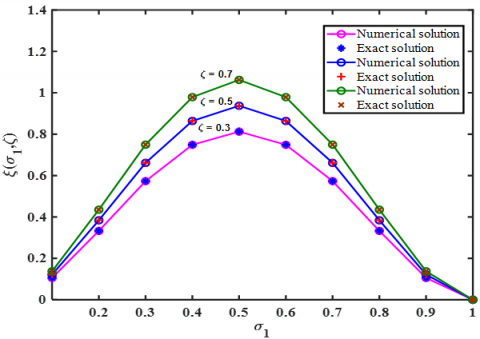
Figure 1 establishes the comparison between the numerical solution and the exact solution for the Numerical Scheme at $\zeta=0.3,0.5,0.7$ when $\gamma=1-0.5 e^{-\sigma_{1} \zeta}, \tau=h=\frac{1}{10} .$ Table 1 demonstrates the absolute value of the maximum errors (MEs) of the numerical solution at $\zeta=1,2,3$.
Figure 1. The numerical solution and exact solutions of equation (12) at $\zeta=0.3,0.5,0.7$
Clearly, we can conclude from Figure 1 that the numerical solutions are excellent consistent with the exact solutions and prove the effectiveness of the proposed method with an error equal zero, see Table 1.
Table 1. MEs of our method at $\zeta=1,2,3$ for example 1
|
h=τ |
ME of our method |
|
1/50 |
0.0000 |
|
1/100 |
0.0000 |
|
1/200 |
0.0000 |
|
1/400 |
0.0000 |
Example 2: Consider the problem equation (1) with the following N-LBCs and IC:
$\beta_{1} D_{\zeta} \Omega\left(\sigma_{1}, \zeta\right)+\beta_{2} D_{+\zeta}^{0.8+0.005 \cos \left(\sigma_{1} \zeta\right) \sin \left(\sigma_{1} \zeta\right)} \Omega\left(\sigma_{1}, \zeta\right)$
$+\beta_{3} D_{-\zeta}^{0.8+0.005 \cos \left(\sigma_{1} \zeta\right) \sin \left(\sigma_{1} \zeta\right)} \Omega\left(\sigma_{1}, \zeta\right)$
$+\beta_{4} D_{\sigma_{1}} \Omega\left(\sigma_{1}, \zeta\right)-\beta_{5} D_{\sigma_{1}}^{2} \Omega\left(\sigma_{1}, \zeta\right)=Q\left(\sigma_{1}, \zeta\right)$ (13)
Subjects to the IC and N-LBCs:
$\Omega\left(\sigma_{1}, 0\right)=5 \sigma_{1}\left[1-\sigma_{1}\right], \quad 0 \leq \sigma_{1} \leq 1$,
$\Omega(0, \zeta)=\int_{0}^{1} \sigma_{1} \cdot \zeta\left[5(\zeta+1) \cdot \sigma_{1}\left(1-\sigma_{1}\right)\right] d \sigma_{1}$
$-\left[\frac{5 \sigma_{1} \cdot \zeta(\zeta+1)}{6} \mid, 0 \leq \zeta \leq J,\right.$,
$\Omega(1, \zeta)=\int_{0}^{1} \sigma_{1} \cdot \zeta\left[5(\zeta+1) \cdot \sigma_{1}\left(1-\sigma_{1}\right)\right] d \sigma_{1}$
$-\left[0.833 \cdot\left(\sigma_{1} \cdot \zeta^{2}+\sigma_{1} \cdot \zeta\right], 0 \leq \zeta \leq J\right.$,
where:
$\begin{aligned} Q\left(\sigma_{1}, \zeta\right) &=(5 \zeta+5)\left(1-\sigma_{1}\right)-(5 \zeta+5) \sigma_{1} \\ &-2(-10 \zeta-10)-5 \sigma_{1}\left(1-\sigma_{1}\right)+5 \sigma_{1}(1\\ & \left.-\sigma_{1}\right)\left(\frac{\zeta^{0.2-0.5 e-2 \cos \left(\sigma_{1} \zeta\right) \sin \left(\sigma_{1}\right)}}{\Gamma\left(2-\zeta^{0.2-0.5 e-2 \cos \left(\sigma_{1} \zeta\right) \sin \left(\sigma_{1}\right)}\right)}\right) \\ &+5 \sigma_{1}(1\\ & \left.-\sigma_{1}\right)\left(\frac{(1-\zeta)^{0.2-0.5 e-2 \cos \left(\sigma_{1} \zeta\right) \sin \left(\sigma_{1}\right)}}{\Gamma\left(2-\zeta^{0.2-0.5 e-2 \cos \left(\sigma_{1} \zeta\right) \sin \left(\sigma_{1}\right)}\right)}\right) \end{aligned}$,
And
$\beta_{1}=\beta_{2}=\beta_{3}=\beta_{4}=\beta_{5}=1$,
The exact solution to this problem is:
$\Omega\left(\sigma_{1}, \zeta\right)=5 \sigma_{1}\left(1-\sigma_{1}\right)(\zeta+1), 0 \leq \sigma_{1} \leq 1$.
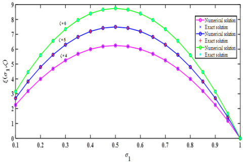
The absolute errors of the numerical solutions, at $\zeta=$ $0.5,0.6, \tau=h=\frac{1}{10} \quad$ and $\quad \alpha\left(\sigma_{1}, \zeta\right)=0.8+$ $0.005 \cos \left(\sigma_{1} \zeta\right) \sin \left(\sigma_{1} \zeta\right)$ are shown in Table 2 . a comparison of the numerical solutions is made by the results reported in proposed method and exact solution. Table 3. demonstrates the absolute value of the maximum errors (MEs) of the numerical solution at $\tau=h=\frac{1}{50}, \frac{1}{100}, \frac{1}{200}, \frac{1}{400}$. Also, the results of the presented method at $\zeta=4,5,6$.
Obviously, we can deduce from Figure 2 that the numerical solutions are excellent agreement with the exact solutions and indicate the effectiveness of the proposed method with an error equal zero, as clarify in Table 2 and Table 3.
Table 2. Some of comparison between exact solution and analytical solution when $\gamma\left(\sigma_{1}, \zeta\right)=0.8+0.005 \cos \left(\sigma_{1} \zeta\right) \sin \left(\sigma_{1} \zeta\right)$ for example, 2
|
$\sigma_{1}$ |
$\zeta$ |
Exact Solution |
Variational Iteration Method |
$\mid \xi_{e x}-\xi_{V I M} \mid$ |
|
0 |
0.5 |
0.000 |
0.000 |
0.000 |
|
0.1 |
0.5 |
0.675 |
0.675 |
0.000 |
|
0.2 |
0.5 |
1.200 |
1.200 |
0.000 |
|
0.3 |
0.5 |
1.575 |
1.575 |
0.000 |
|
0.4 |
0.5 |
1.800 |
1.800 |
0.000 |
|
0.5 |
0.5 |
1.875 |
1.875 |
0.000 |
|
0.6 |
0.5 |
1.800 |
1.800 |
0.000 |
|
0.7 |
0.5 |
1.575 |
1.575 |
0.000 |
|
0.8 |
0.5 |
1.200 |
1.200 |
0.000 |
|
0.9 |
0.5 |
0.675 |
0.675 |
0.000 |
|
1 |
0.5 |
0.000 |
0.000 |
0.000 |
|
0 |
0.6 |
0.000 |
0.000 |
0.000 |
|
0.1 |
0.6 |
0.720 |
0.720 |
0.000 |
|
0.2 |
0.6 |
1.280 |
1.280 |
0.000 |
|
0.3 |
0.6 |
1.680 |
1.680 |
0.000 |
|
0.4 |
0.6 |
1.920 |
1.920 |
0.000 |
|
0.5 |
0.6 |
2.000 |
2.000 |
0.000 |
|
0.6 |
0.6 |
1.920 |
1.920 |
0.000 |
|
0.7 |
0.6 |
1.680 |
1.680 |
0.000 |
|
0.8 |
0.6 |
1.280 |
1.280 |
0.000 |
|
0.9 |
0.6 |
0.720 |
0.720 |
0.000 |
|
1 |
0.6 |
0.000 |
0.000 |
0.000 |
Table 3. MEs of our method at $\zeta=4,5,6$ for example 2
|
h=τ |
MEs of our method |
|
1/50 |
0.0000 |
|
1/100 |
0.0000 |
|
1/200 |
0.0000 |
|
1/400 |
0.0000 |
Figure 2. The numerical solution and exact solutions $\Omega\left(\sigma_{1}, \zeta\right)$ of Eq. (13)
Example 3: Consider the problem Eq. (1) with the following IC and N-LBCs:
$\begin{aligned} \beta_{1} D_{\zeta} \Omega\left(\sigma_{1}, \sigma_{2},\right.&\zeta)+\beta_{2} D_{+\zeta}^{1-0.5 e^{-\sigma_{1}, \sigma_{2} \zeta}} \Omega\left(\sigma_{1}, \sigma_{2}, \zeta\right) \\ &+\beta_{3} D_{-\zeta}^{1-0.5 e^{-\sigma_{1}, \sigma_{2} \zeta}} \Omega\left(\sigma_{1}, \sigma_{2}, \zeta\right) \\ &=-\beta_{4} D_{\sigma_{1}} \Omega\left(\sigma_{1}, \sigma_{2}, \zeta\right) \\ &-\beta_{4} D_{\sigma_{2}} \Omega\left(\sigma_{1}, \sigma_{2}, \zeta\right) \\ &+\beta_{5} D_{\sigma_{1}}^{2} \Omega\left(\sigma_{1}, \sigma_{2}, \zeta\right) \\ &+\beta_{5} D_{\sigma_{2}}^{2} \Omega\left(\sigma_{1}, \sigma_{2}, \zeta\right) \\ &+Q\left(\sigma_{1}, \sigma_{2}, \zeta\right), \end{aligned}$ (14)
Subjects to the IC and N-LBCs:
$\Omega\left(\sigma_{1}, \sigma_{2}, 0\right)=10 \sigma_{1}^{2} \sigma_{2}^{2}\left(1-\sigma_{1}\right)^{2}\left(1-\sigma_{2}\right)^{2}0 \leq \sigma_{1}, \sigma_{2} \leq 1$
$\Omega\left(0, \sigma_{2}, \zeta\right)=\int_{0}^{1} \sigma_{1}^{2}\left(10 \sigma_{1}^{2} \cdot \zeta^{2}\left(1-\sigma_{1}\right)^{2}\left(1-\sigma_{2}\right)^{2}(1+\zeta)\right) d \sigma_{1}-\left(\frac{2 \sigma_{2}^{2}\left(1-\sigma_{2}\right)^{2}(1+\zeta)}{21}\right)$,
$\Omega\left(\sigma_{1}, 0, \zeta\right)=\int_{0}^{1} \sigma_{1}^{2}\left(10 \sigma_{1}^{2} \cdot \zeta^{2}\left(1-\sigma_{1}\right)^{2}\left(1-\sigma_{2}\right)^{2}(1+\zeta)\right) d \sigma_{2}-\left(\frac{\sigma_{2}\left(1-\sigma_{1}\right)^{2}(1+\zeta)}{3}\right)$
$\Omega\left(1, \sigma_{2}, \zeta\right)=\int_{0}^{1} \sigma_{1}^{2}\left(10 \sigma_{1}^{2} \zeta^{2}\left(1-\sigma_{1}\right)^{2}\left(1-\sigma_{2}\right)^{2}(1+\zeta)\right) d \sigma_{1}-\left(0.095\left(1-\sigma_{2}\right)^{2}\left(\sigma_{2}^{2}+\zeta \sigma_{2}^{2}\right)\right)$
$\quad \Omega\left(\sigma_{1}, 1, \zeta\right)=\int_{0}^{1} \sigma_{1}^{2}\left(\begin{array}{c}10 \sigma_{1}{ }^{2} \zeta^{2}\left(1-\sigma_{1}\right)^{2}\left(1-\sigma_{2}\right)^{2} \\ (1+\zeta)\end{array}\right) d \sigma_{2}-\left(0.3 \sigma_{2}\left(1-\sigma_{1}\right)^{2}(1+\zeta)\right), 0 \leq \zeta \leq J$,
where:
$\begin{aligned} Q\left(\sigma_{1}, \sigma_{2}, \zeta\right)=2 \sigma_{1}, \sigma_{2}^{2}(10 \zeta+10)\left(1-\sigma_{1}\right)^{2}\left(1-\sigma_{2}\right)^{2} \\ &-2 \sigma_{1}^{2} \sigma_{2}^{2}(10 \zeta+10)\left(1-\sigma_{1}\right)\left(1-\sigma_{2}\right)^{2} \\ &-2 \sigma_{2}^{2}(10+10)\left(1-\sigma_{1}\right)^{2}\left(1-\sigma_{2}\right)^{2} \\ &-8 \sigma_{1} \sigma_{2}^{2}(10 \zeta+10)\left(1-\sigma_{1}\right)\left(1-\sigma_{2}\right)^{2} \\ &+2 \sigma_{1}^{2} \sigma_{2}^{2}(10 \zeta+10)\left(1-\sigma_{2}\right)^{2} \\ &+2 \sigma_{1}^{2} \sigma_{2}(10 \zeta+10)\left(1-\sigma_{1}\right)^{2}\left(1-\sigma_{2}\right)^{2} \\ &-2 \sigma_{1}^{2} \sigma_{2}^{2}(10 \zeta+10)\left(1-\sigma_{1}\right)^{2}\left(1-\sigma_{2}\right) \\ &+2 \sigma_{1}^{2}(10 \zeta+10)\left(1-\sigma_{1}\right)^{2}\left(1-\sigma_{2}\right)^{2} \\ &+2 \sigma_{1}^{2} \sigma_{2}(10 \zeta+10)\left(1-\sigma_{1}\right)^{2}\left(1-\sigma_{2}\right) \\ &+2 \sigma_{1}^{2} \sigma_{2}^{2}(10 \zeta+10)\left(1-\sigma_{1}\right)^{2} \\ &+10 \sigma_{1}{ }^{2} \sigma_{2}{ }^{2}\left(1-\sigma_{1}\right)^{2}\left(1-\sigma_{2}\right)^{2} \\ &+10 \sigma_{1}{ }^{2} \sigma_{2}{ }^{2}\left(1-\sigma_{1}\right)^{2}(1\\ & \left.-\sigma_{2}\right)^{2}\left(\frac{\zeta^{5 e^{-\sigma_{1}, \sigma_{2} \zeta}}}{\Gamma\left(1+5 e^{-\sigma_{1}, \sigma_{2} \zeta}\right)}\right) \\ &+10 \sigma_{1}^{2} \sigma_{2}^{2}\left(1-\sigma_{1}\right)^{2}(1\\ & \left.-\sigma_{2}\right)^{2}\left(\frac{(1-\zeta)^{5 e^{-\sigma_{1}, \sigma_{2} \zeta}}}{\Gamma\left(1+5 e^{-\sigma_{1}, \sigma_{2} \zeta}\right)}\right) \end{aligned}$,
and
$\beta_{1}=\beta_{2}=\beta_{3}=\beta_{4}=\beta_{5}=1$,
that the exact solution to this problem is:
$\Omega\left(\sigma_{1}, \sigma_{2}, \zeta\right)=10 \sigma_{1}^{2} \sigma_{2}^{2}\left(1-\sigma_{1}\right)^{2}\left(1-\sigma_{2}\right)^{2}(1+\zeta)0 \leq \sigma_{1}, \sigma_{2} \leq 1$.
Some of comparison between exact solution and proposed method for VFOMADM with 2-D at $\zeta=4,5,6, \tau=h=\frac{1}{10}$ and $\alpha\left(\sigma_{1}, \sigma_{2}, \zeta\right)=1-0.5 e^{-\sigma_{1}, \sigma_{2} \zeta}$, are shown in Table 4 with an error equal zero. In addition to, the absolute values of the MEs of the numerical solution at $\zeta=1,2,3$ are shown in Table 5 with an error equal zero.
Table 4. Some of comparison between exact solution and analytical solution when $\alpha\left(\sigma_{1}, \sigma_{2}, \zeta\right)=1-0.5 \mathrm{e}^{-\sigma_{1}, \sigma_{2} \zeta}$ for example 3
|
$\sigma_{1}=\sigma_{2}$ |
$\zeta$ |
Exact Solution |
Variational Iteration Method |
$\left|\xi_{e x}-\xi_{V I M}\right|$ |
|
0 |
4 |
0.000 |
0.000 |
0.000 |
|
0.1 |
4 |
6.561×10⁻⁴ |
6.561×10⁻⁴ |
0.000 |
|
0.2 |
4 |
6.554×10⁻³ |
6.554×10⁻³ |
0.000 |
|
0.3 |
4 |
0.019 |
0.019 |
0.000 |
|
0.4 |
4 |
0.033 |
0.033 |
0.000 |
|
0.5 |
4 |
0.039 |
0.039 |
0.000 |
|
0.6 |
4 |
0.033 |
0.033 |
0.000 |
|
0.7 |
4 |
0.019 |
0.019 |
0.000 |
|
0.8 |
4 |
6.554×10⁻³ |
6.554×10⁻³ |
0.000 |
|
0.9 |
4 |
6.561×10⁻⁴ |
6.561×10⁻⁴ |
0.000 |
|
1 |
4 |
0.000 |
0.000 |
0.000 |
|
0 |
5 |
0.000 |
0.000 |
0.000 |
|
0.1 |
5 |
6.561×10⁻⁴ |
6.561×10⁻⁴ |
0.000 |
|
0.2 |
5 |
6.554×10⁻³ |
6.554×10⁻³ |
0.000 |
|
0.3 |
5 |
0.019 |
0.019 |
0.000 |
|
0.4 |
5 |
0.033 |
0.033 |
0.000 |
|
0.5 |
5 |
0.039 |
0.039 |
0.000 |
|
0.6 |
5 |
0.033 |
0.033 |
0.000 |
|
0.7 |
5 |
0.019 |
0.019 |
0.000 |
|
0.8 |
5 |
6.554×10⁻³ |
6.554×10⁻³ |
0.000 |
|
0.9 |
5 |
6.561×10⁻⁴ |
6.561×10⁻⁴ |
0.000 |
|
1 |
5 |
0.000 |
0.000 |
0.000 |
|
0 |
6 |
0.000 |
0.000 |
0.000 |
|
0.1 |
6 |
6.561×10⁻⁴ |
6.561×10⁻⁴ |
0.000 |
|
0.2 |
6 |
6.554×10⁻³ |
6.554×10⁻³ |
0.000 |
|
0.3 |
6 |
0.019 |
0.019 |
0.000 |
|
0.4 |
6 |
0.033 |
0.033 |
0.000 |
|
0.5 |
6 |
0.039 |
0.039 |
0.000 |
|
0.6 |
6 |
0.033 |
0.033 |
0.000 |
|
0.7 |
6 |
0.019 |
0.019 |
0.000 |
|
0.8 |
6 |
6.554×10⁻³ |
6.554×10⁻³ |
0.000 |
|
0.9 |
6 |
6.561×10⁻⁴ |
6.561×10⁻⁴ |
0.000 |
|
1 |
6 |
0.000 |
0.000 |
0.000 |
Table 5. MEs of the numerical solution at $\zeta$=1,2,3 for example 3
|
h=τ |
MEs of our method |
|
1/50 |
0.0000 |
|
1/100 |
0.0000 |
|
1/200 |
0.0000 |
|
1/400 |
0.0000 |
Example 4: Consider the problem Eq. (1) with the following N-LBCs and IC:
$\beta_{1} D_{\zeta} \Omega\left(\sigma_{1}, \sigma_{2}, \zeta\right)$
$+\beta_{2} D_{+\zeta}^{0.8+0.005 \cos \left(\sigma_{1}, \sigma_{2} \zeta\right) \sin \left(\sigma_{1}, \sigma_{2}\right)} \Omega\left(\sigma_{1}, \sigma_{2}, \zeta\right)$
$+\beta_{3} D_{-\zeta}^{0.8+0.005 \cos \left(\sigma_{1}, \sigma_{2} \zeta\right) \sin \left(\sigma_{1}, \sigma_{2}\right)} \Omega\left(\sigma_{1}, \sigma_{2}, \zeta\right)$
$=-\beta_{4} D_{\sigma_{1}} \Omega\left(\sigma_{1}, \sigma_{2}, \zeta\right)-\beta_{4} D_{\sigma_{2}} \Omega\left(\sigma_{1}, \sigma_{2}, \zeta\right)$
$+\beta_{5} D_{\sigma_{1}}^{2} \Omega\left(\sigma_{1}, \sigma_{2}, \zeta\right)+\beta_{5} D_{\sigma_{2}}^{2} \Omega\left(\sigma_{1}, \sigma_{2}, \zeta\right)$
$+Q\left(\sigma_{1}, \sigma_{2}, \zeta\right)$ (15)
Subjects to the IC and N-LBCs:
$\Omega\left(\sigma_{1}, \sigma_{2}, 0\right)=5 \sigma_{1}\left(1-\sigma_{1}\right)\left(1-\sigma_{2}\right), \quad 0 \leq \sigma_{1}, \sigma_{2} \leq 1$
$\Omega\left(0, \sigma_{2}, \zeta\right)=\int_{0}^{1} \sigma_{1}^{2}\left(5 \sigma_{1} \sigma_{2} \zeta\left(1-\sigma_{1}\right)\left(1-\sigma_{2}\right)(1+\zeta)\right) d \sigma_{1}+\left(\frac{\sigma_{2}\left(\sigma_{2}-1\right)(1+\zeta)}{6}\right)$,
$\Omega\left(\sigma_{1}, 0, \zeta\right)=\int_{0}^{1} \sigma_{1}^{2}\left(5 \sigma_{1} \sigma_{2} \zeta\left(1-\sigma_{1}\right)\left(1-\sigma_{2}\right)(1+\zeta)\right) d \sigma_{2}+\left(\frac{5 \sigma_{1}^{4}\left(\sigma_{1}-1\right)(1+\zeta)}{6}\right)$,
$\Omega\left(1, \sigma_{2}, \zeta\right)=\int_{0}^{1} \sigma_{1}^{2}\left(5 \sigma_{1} \sigma_{2} \zeta\left(1-\sigma_{1}\right)\left(1-\sigma_{2}\right)(1+\zeta)\right) d \sigma_{1}+0.167\left(\sigma_{2}-1\right)\left(\sigma_{2}+\zeta \sigma_{2}\right)$
$\Omega\left(\sigma_{1}, 1, \zeta\right)=\int_{0}^{1} \sigma_{1}^{2}\left(5 \sigma_{1} \sigma_{2} \zeta\left(1-\sigma_{1}\right)\left(1-\sigma_{2}\right)(1+\zeta)\right) d \sigma_{2}+0.833\left(\sigma_{1}-1\right)\left(\sigma_{1}^{4}+\zeta \sigma_{1}^{4}\right)0 \leq \zeta \leq J$
where,
$Q\left(\sigma_{1}, \sigma_{2}, \zeta\right)$
$=2 \sigma_{1} \sigma_{2}(5 \zeta+5)\left(1-\sigma_{1}\right)\left(1-\sigma_{2}\right)-\sigma_{1}^{2} \sigma_{2}(5 \zeta+5)(1$
$\left.-\sigma_{2}\right)+\sigma_{1}^{2}(5 \zeta+5)\left(1-\sigma_{1}\right)\left(1-\sigma_{2}\right)-\sigma_{1}^{2} \sigma_{2}(5 \zeta+5)(1$
$\left.-\sigma_{1}\right)-2 \sigma_{2}(5 \zeta+5)\left(1-\sigma_{1}\right)\left(1-\sigma_{2}\right)+4 \sigma_{1}, \sigma_{1}(5 \zeta+5)(1$
$\left.-\sigma_{2}\right)+2 \sigma_{1}{ }^{2}(5 \zeta+5)\left(1-\sigma_{1}\right)+5 \sigma_{1}{ }^{2} \sigma_{2}\left(1-\sigma_{1}\right)\left(1-\sigma_{2}\right)$
$+5 \sigma_{1}, \sigma_{2}\left(1-\sigma_{1}\right)(1$
$\left.-\sigma_{2}\right)\left(\frac{\zeta^{0.2-0.5 e-2 \cos \left(\sigma_{1}, \sigma_{2} \zeta\right) \sin \left(\sigma_{1}, \sigma_{2}\right)}}{\Gamma\left(2-\zeta^{0.2-0.5 e-2 \cos \left(\sigma_{1}, \sigma_{2} \zeta\right) \sin \left(\sigma_{1}, \sigma_{2}\right)}\right)}\right)+5 \sigma_{1}, \sigma_{2}(1$
$\left.-\sigma_{1}\right)\left(1-\sigma_{2}\right)\left(\frac{(1-\zeta)^{0.2-0.5 e-2 \cos \left(\sigma_{1}, \sigma_{2} \zeta\right) \sin \left(\sigma_{1}, \sigma_{2}\right)}}{\Gamma\left(2-\zeta^{0.2-0.5 e-2 \cos \left(\sigma_{1}, \sigma_{2} \zeta\right) \sin \left(\sigma_{1}, \sigma_{2}\right)}\right)}\right)$,
And
$\beta_{1}=\beta_{2}=\beta_{3}=\beta_{4}=\beta_{5}=1$,
The exact solution to this problem is:
$\Omega\left(\sigma_{1}, \sigma_{2}, \zeta\right)=5 \sigma_{1}, \sigma_{2}\left(1-\sigma_{1}\right)\left(1-\sigma_{2}\right)(\zeta+1), 0 \leq \sigma_{1}, \sigma_{2} \leq 1$.
The absolute value of the MEs of the numerical solution at $\zeta=1,2,3$ with an error equal zero (Table 6). Moreover, Table 7 demonstrates the comparison between the numerical solution and the exact solution at at $\zeta=4,5,6, \tau=h=\frac{1}{10}$ and $\alpha\left(\sigma_{1}, \sigma_{2}, \zeta\right)=1-0.5 e^{-\sigma_{1}, \sigma_{2} \zeta}$ with an error equal zero.
Table 6. MEs of the numerical solution at $\zeta=4,5,6$ for example 4
|
h=τ |
MEs of our method |
|
0.200 |
0.0000 |
|
0.100 |
0.0000 |
|
0.050 |
0.0000 |
|
0.025 |
0.0000 |
Table 7. Some of comparison between exact solution and analytical solution when $\alpha\left(\sigma_{1}, \sigma_{2}, \zeta\right)=0.8+0.005 \cos \left(\sigma_{1}, \sigma_{2} \zeta\right) \sin \left(\sigma_{1}, \sigma_{2}\right)$ for example 4
|
$\sigma_{1}=\sigma_{2}$ |
$\zeta$ |
Exact Solution |
Variational Iteration Method |
$\left|\xi_{e x}-\xi_{V I M}\right|$ |
|
0 |
1 |
0.0000 |
0.0000 |
0.000 |
|
0.1 |
1 |
0.0081 |
0.0081 |
0.000 |
|
0.2 |
1 |
0.0512 |
0.0512 |
0.000 |
|
0.3 |
1 |
0.1323 |
0.1323 |
0.000 |
|
0.4 |
1 |
0.2304 |
0.2304 |
0.000 |
|
0.5 |
1 |
0.3125 |
0.3125 |
0.000 |
|
0.6 |
1 |
0.3456 |
0.3456 |
0.000 |
|
0.7 |
1 |
0.3087 |
0.3087 |
0.000 |
|
0.8 |
1 |
0.2048 |
0.2048 |
0.000 |
|
0.9 |
1 |
0.0730 |
0.0730 |
0.000 |
|
1 |
1 |
0.0000 |
0.0000 |
0.000 |
|
0 |
2 |
0.0000 |
0.0000 |
0.000 |
|
0.1 |
2 |
0.0120 |
0.0120 |
0.000 |
|
0.2 |
2 |
0.0768 |
0.0768 |
0.000 |
|
0.3 |
2 |
0.1985 |
0.1985 |
0.000 |
|
0.4 |
2 |
0.3456 |
0.3456 |
0.000 |
|
0.5 |
2 |
0.4688 |
0.4688 |
0.000 |
|
0.6 |
2 |
0.5184 |
0.5184 |
0.000 |
|
0.7 |
2 |
0.4631 |
0.4631 |
0.000 |
|
0.8 |
2 |
0.3072 |
0.3072 |
0.000 |
|
0.9 |
2 |
0.1094 |
0.1094 |
0.000 |
|
1 |
2 |
0.0000 |
0.0000 |
0.000 |
Three main objectives were achieved in this work started from presenting mixed initial and boundary conditions are used to modify the treatment of initial boundary conditions. of TSMDVOF-MIDENLCB then explaining an alternative approach for proposed problems of the variational iteration method. Finally, studying the method of convergence and addressing the condition of sufficient for convergence. In addition, we got for each iteration, a new initial solution and conclude this system was fast to reach the exact value when mixed initial and boundary togethared using fractional variatinal iteration method in terms of execution time. This algorithm was simple and easy to implement. Moreover, successfully applied the given approach for solving various TSMDVOF-MIDENLCB classes. The efficiency and the accuracy of the suggested method clarified from the observation of all simulation results and numerical examples.
|
TSMDVOF-MIDENLCs |
Two-sided multi-dimensional variable order fractional mobile/ immobile diffusion equation with non-local conditions |
|
SC |
Sufficient conditions |
|
FDEs |
Fractional partial differential equations |
|
IC |
initial condition |
|
N-LBCs |
Non-local boundary conditions |
|
FVIM |
Fractional variational iteration method |
|
$\mathrm{E}_{j}(x, t)$ |
maximum error |
|
Greek symbols |
|
|
$\varphi\left(\sigma_{1}, \sigma_{2}, \ldots, \sigma_{n}, \zeta\right)$, $L_{n}\left(\sigma_{1}, \sigma_{2}, \ldots, \sigma_{n}, \zeta\right)$, $Q\left(\sigma_{1}, \sigma_{2}, \ldots, \sigma_{n}, \zeta\right)$, $M_{n}\left(\sigma_{1}, \sigma_{2}, \ldots, \sigma_{n}, \zeta\right)$ |
Function of known $\sigma_{n}$ and $\zeta$ |
|
$\Omega_{n}^{*}$ |
New successive initial solution |
|
$\lambda$ |
Multiplier of Lagrangian |
[1] Ismaeelpour, T., Hemmat, A.A., Saeedi, H. (2017). B-spline operational matrix of fractional integration. Optik, 130: 291-305. https://doi.org/10.1016/j.ijleo.2016.10.066
[2] Khan, RA., Khalil, H. (2014). A new method based on Legendre polynomials for solution of system of fractional order partial differential equations. Inter. Jour. of Comp. Math, 91(12): 2554-67. https://doi.org/10.1080/00207160.2014.880781
[3] Moghadam, M.M., Saeedi, H., Mollahasani, N. (2010). A new operational method for solving nonlinear Volterra integro-differential equations with fractional order. Jour. of Infor. & Math. Sci., 2(2 & 3): 95-107.
[4] Saeedi, H. (2017). The linear b-spline scaling function operational matrix of fractional integration and its applications in solving fractional-order differential equations. Iranian Journal of Science and Technology, Transactions A: Science, 41(3): 723-733.
[5] Baleanu, D., Diethelm, K., Scalas, E., Trujillo, J.J. (2012). Fractional Calculus: Models and Numerical Methods. https://doi.org/10.1142/8180
[6] Liu, F., Zhuang, P., Liu, Q. (2015). Numerical methods of Fractional Partial Differential Equations and Applications. Science Press, China.
[7] Gorial, I.I. (2013). Analytical solution for two-dimensional fractional dispersion equation by modified decomposition method. World Applied Sciences Journal, 23(8): 1049-1052. https://doi.org/10.5829/idosi.wasj.2013.23.08.2578
[8] Ding, X.L., Nieto, J.J. (2017). Analytical solutions for coupling fractional partial differential equations with Dirichlet boundary conditions. Communications in Nonlinear Science and Numerical Simulation, 52: 165-176. https://doi.org/10.1016/j.cnsns.2017.04.020
[9] Gorial, I.I. (2012). A semi-analytic method for solving partial differential equations with non-local boundary conditions. Journals of Sci. & Eng. Rese, 5(7): 293-296.
[10] Gorial, I.I. (2012). On the numerical solution of the 3-dimensional fractional diffusion equation in the shifted grunwald estimate form. Int. J. Modern Math. Sci, 1(3): 121-133.
[11] Wei, S., Chen, W., Hon, Y.C. (2016). Characterizing time dependent anomalous diffusion process: A survey on fractional derivative and nonlinear models. Physica A: Statistical Mechanics and its Applications, 462: 1244-1251. https://doi.org/10.1016/j.physa.2016.06.145
[12] Chen, C.M., Liu, F., Burrage, K. (2008). Finite difference methods and a Fourier analysis for the fractional reaction–subdiffusion equation. Applied Mathematics and Computation, 198(2): 754-769. https://doi.org/10.1016/j.amc.2007.09.020
[13] Li, C., Zhao, Z., Chen, Y. (2011). Numerical approximation of nonlinear fractional differential equations with subdiffusion and superdiffusion. Computers & Mathematics with Applications, 62(3): 855-875. https://doi.org/10.1016/j.camwa.2011.02.045
[14] Liu, F., Zhuang, P., Burrage, K. (2012). Numerical methods and analysis for a class of fractional advection–dispersion models. Computers & Mathematics with Applications, 64(10): 2990-3007. https://doi.org/10.1016/j.camwa.2012.01.020
[15] Ma, H., Yang, Y. (2016). Jacobi spectral collocation method for the time variable-order fractional mobile-immobile advection-dispersion solute transport model. East Asian Journal on Applied Mathematics, 6(3): 337-352. https://doi.org/10.4208/eajam.141115.060616a
[16] Meerschaert, M.M., Tadjeran, C. (2004). Finite difference approximations for fractional advection–dispersion flow equations. Journal of Computational and Applied Mathematics, 172(1): 65-77. https://doi.org/10.1016/j.cam.2004.01.033
[17] Schumer, R., Benson, D.A., Meerschaert, M.M., Baeumer, B. (2003). Fractal mobile/immobile solute transport. Water Resources Research, 39(10). https://doi.org/10.1029/2003WR002141
[18] Yu, B., Jiang, X., Xu, H. (2015). A novel compact numerical method for solving the two-dimensional non-linear fractional reaction-subdiffusion equation. Numerical Algorithms, 68(4): 923-950. https://doi.org/10.1007/s11075-014-9877-1
[19] Zhang, H., Liu, F., Phanikumar, M.S., Meerschaert, M.M. (2013). A novel numerical method for the time variable fractional order mobile–immobile advection–dispersion model. Computers & Mathematics with Applications, 66(5): 693-701. https://doi.org/10.1016/j.camwa.2013.01.031
[20] Abdelkawy, M.A., Zaky, M.A., Bhrawy, A.H., Baleanu, D. (2015). Numerical simulation of time variable fractional order mobile-immobile advection-dispersion model. Rom. Rep. Phys, 67(3): 773-791.
[21] Cheng, J., Nakagawa, J., Yamamoto, M., Yamazaki, T. (2009). Uniqueness in an inverse problem for a one-dimensional fractional diffusion equation. Inverse Problems, 25(11): 115002. https://doi.org/10.1088/0266-5611/25/11/115002
[22] Meerschaert, M.M., Tadjeran, C. (2006). Finite difference approximations for two-sided space-fractional partial differential equations. Applied Numerical Mathematics, 56(1): 80-90. https://doi.org/10.1016/j.apnum.2005.02.008
[23] Ding, Z., Xiao, A., Li, M. (2010). Weighted finite difference methods for a class of space fractional partial differential equations with variable coefficients. Journal of Computational and Applied Mathematics, 233(8): 1905-1914. https://doi.org/10.1016/j.cam.2009.09.027
[24] Wang, H., Du, N. (2014). Fast alternating-direction finite difference methods for three-dimensional space-fractional diffusion equations. Journal of Computational Physics, 258: 305-318. https://doi.org/10.1016/j.jcp.2013.10.040
[25] Ma, J., Liu, J., Zhou, Z. (2014). Convergence analysis of moving finite element methods for space fractional differential equations. Journal of Computational and Applied Mathematics, 255: 661-670. https://doi.org/10.1016/j.cam.2013.06.021
[26] Zhang, H., Liu, F., Anh, V. (2010). Galerkin finite element approximation of symmetric space-fractional partial differential equations. Applied Mathematics and Computation, 217(6): 2534-2545. https://doi.org/10.1016/j.amc.2010.07.066
[27] Li, L., Xu, D., Luo, M. (2013). Alternating direction implicit Galerkin finite element method for the two-dimensional fractional diffusion-wave equation. Journal of Computational Physics, 255: 471-485. https://doi.org/10.1016/j.jcp.2013.08.031
[28] Lorenzo, C.F., Hartley, T.T. (2002). Variable order and distributed order fractional operators. Nonlinear Dynamics, 29(1): 57-98. https://doi.org/10.1023/A:1016586905654
[29] Ingman, D., Suzdalnitsky, J. (2004). Control of damping oscillations by fractional differential operator with time-dependent order. Computer Methods in Applied Mechanics and Engineering, 193(52): 5585-5595. https://doi.org/10.1016/j.cma.2004.06.029
[30] Pedro, H.T.C., Kobayashi, M.H., Pereira, J.M.C., Coimbra, C.F.M. (2008). Variable order modeling of diffusive-convective effects on the oscillatory flow past a sphere. Journal of Vibration and Control, 14(9-10): 1659-1672. https://doi.org/10.1177/1077546307087397
[31] Ramirez, L.E., Coimbra, C.F. (2010). On the selection and meaning of variable order operators for dynamic modeling. International Journal of Differential Equations. https://doi.org/10.1155/2010/846107
[32] Lin, R., Liu, F., Anh, V., Turner, I. (2009). Stability and convergence of a new explicit finite-difference approximation for the variable-order nonlinear fractional diffusion equation. Applied Mathematics and Computation, 212(2): 435-445. https://doi.org/10.1016/j.amc.2009.02.047
[33] Zhuang, P., Liu, F., Anh, V., Turner, I. (2009). Numerical methods for the variable-order fractional advection-diffusion equation with a nonlinear source term. SIAM Journal on Numerical Analysis, 47(3): 1760-1781. https://doi.org/10.1137/080730597
[34] Chen, C.M., Liu, F., Anh, V., Turner, I. (2010). Numerical schemes with high spatial accuracy for a variable-order anomalous subdiffusion equation. SIAM Journal on Scientific Computing, 32(4): 1740-1760. https://doi.org/10.1137/090771715
[35] Chen, Y.M., Wei, Y.Q., Liu, D.Y., Yu, H. (2015). Numerical solution for a class of nonlinear variable order fractional differential equations with Legendre wavelets. Applied Mathematics Letters, 46: 83-88. https://doi.org/10.1016/j.aml.2015.02.010
[36] Shen, S., Liu, F., Chen, J., Turner, I., Anh, V. (2012). Numerical techniques for the variable order time fractional diffusion equation. Applied Mathematics and Computation, 218(22): 10861-10870. https://doi.org/10.1016/j.amc.2012.04.047
[37] Shen, S., Liu, F., Anh, V., Turner, I., Chen, J. (2013). A characteristic difference method for the variable-order fractional advection-diffusion equation. Journal of Applied Mathematics and Computing, 42(1): 371-386. https://doi.org/10.1007/s12190-012-0642-0
[38] Zhao, X., Sun, Z.Z., Karniadakis, G.E. (2015). Second-order approximations for variable order fractional derivatives: algorithms and applications. Journal of Computational Physics, 293: 184-200. https://doi.org/10.1016/j.jcp.2014.08.015
[39] Sakar, M.G., Ergören, H. (2015). Alternative variational iteration method for solving the time-fractional Fornberg–Whitham equation. Applied Mathematical Modelling, 39(14): 3972-3979. https://doi.org/10.1016/j.apm.2014.11.048
[40] Odibat, Z.M. (2010). A study on the convergence of variational iteration method. Mathematical and Computer Modelling, 51(9-10): 1181-1192. https://doi.org/10.1016/j.mcm.2009.12.034