Mohammad J. Ben Salamah* | Mehmet Savsar
© 2021 IIETA. This article is published by IIETA and is licensed under the CC BY 4.0 license (http://creativecommons.org/licenses/by/4.0/).
OPEN ACCESS
Large flowmeters are used in many industrial facilities, including power plants, cooling-water stations for refineries, and petrochemical plants. These flowmeters are employed for various purposes, including billing. Just like all machines, flowmeters are subject to failure. Drift is a particular type of failure in which the flowmeter produces an error in measurement that would incrementally increase with time.
Maintenance technicians calibrate and fix all measuring equipment, including flowmeters. Nevertheless, downsizing policies and budget cuts in most contemporary industrial facilities have made these technicians overwhelmed with work. A mathematical and computer-based drift-detection scheme is developed to reduce the burden of the maintenance staff. The detection scheme only uses the flowmeter's flow data and the discrete Fourier transform (DFT).
The detection scheme was applied over the flow data from an actual flowmeter that drifted during its operation. DFT application over the data produced by the flowmeter led to expected results and other unexpected results. This paper discusses both results and suggests areas for further study. Practically speaking, the scheme would facilitate the early detection of drifts in flowmeters having seasonal flow regardless of type or manufacturer.
discrete Fourier transform (DFT), flowmeter, instrumentation, instrument drift, measurement quality, metrology
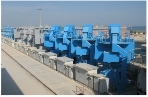
Refineries and petrochemical plants produce large amounts of heat in their operations. This heat must be removed, or else the plants would fail. Large quantities of water are pumped to heat exchangers from cooling pumping stations to remove the heat produced. Figure 1 shows a part of a cooling pumping station.
Figure 1. Part of the pumping station under study
Measuring the quantity of water supplied by the pumping station to its consumers is extremely important because it is used for billing.
A flowmeter measures the amount of water provided to a consumer (plant). Flowmeters, however, are machines, and all machines are subject to failure. If a flowmeter produces an inaccurate reading, the bill sent to the consuming plant would be wrong.
From a managerial point of view, a failing flowmeter is equivalent to money loss. Therefore, a solution must be reached to prevent this loss. Also, management would insist that the cost of such a solution would be as low as possible.
The first line of defense against a flowmeter producing inaccurate readings is the design and manufacturing of the flowmeter. The proper selection and installation of a flowmeter is the second issue to consider when guarding against inaccurate readings. The third line of defense is the correct and timely maintenance and calibration of flowmeters. This activity is where end-users might face some difficulties: Downsizing and the continuous pressure from top management to make more profit with fewer costs led to reduced maintenance staff. Fewer and fewer engineers and technicians must do more and more work with an increasing amount of equipment. In such a case, the emphasis would be on either life-critical equipment or production-critical equipment. A flowmeter is neither. For maintenance staff, a solution to flowmeter inaccuracy should move away from the routine calibration/maintenance model towards a condition-based monitoring model.
There are many types of flowmeters working on different physical principles. Consequently, the electric and electronic circuitry would be different (in principle) for each class. Also, for every type of flowmeter, different manufacturers would produce different circuitry. Therefore, a general solution for detecting flowmeter inaccuracy should be independent of the electrical and electronic circuitry used in a flowmeter.
One general solution to detecting flowmeter inaccuracy would be to observe the pattern of the flow data produced. Then, one should examine its statistical and mathematical properties, looking for abnormalities. Data generated over time is called a time series. The sort of flowmeter inaccuracy or fault that is the subject of this paper is drift. Hence, the general solution should detect drift just from observing the time series of water consumption generated by the flowmeter. This general solution would require entering the data into a computer and analyzing it by software, satisfying management's desire for a solution requiring a minimum cost.
The discrete Fourier transform is one of many methods of analyzing a time series. The Fourier transform (as its name indicates) will 'transform' the time series from the time domain to the frequency domain. What is implied in the Fourier transform is that a (possibly complicated) single series in the time domain is composed of many simple sinusoidal series in the frequency domain. The strength or amplitude of each of these sinusoidal series in the frequency domain is called an ordinate. Many ordinates are representing different frequencies, and they are plotted in a graph called a periodogram. The first ordinate in a periodogram will increase if there is a trend in the original series in the time domain.
The peak of an ordinate in a periodogram would increase or decrease, but its increase or decrease might not be significant. Fisher's test of significance measures the statistical significance of a peak of an ordinate in a periodogram.
The assumption made in this research is that if drift occurs in a flowmeter, the amplitude (or peak) of the first ordinate of the discrete Fourier transform of the time-series of the recorded data would increase and become more extensive than the rest of the ordinates. It is also assumed that when the first ordinate passes the threshold determined by Fisher's test, this would be a clear indication that the flowmeter is drifting.
In a concise statement, this research aims to detect flowmeter drift just by observing the data produced by the flowmeter and analyzing this data by the discrete Fourier transform (DFT).
This research is an attempt at improvement for a previous detection scheme mentioned in the literature. The last method, suggested by Ben Salamah et al. used statistical process control (SPC) to detect drift. As a subject for future studies, the previously mentioned paper suggested finding ways to shorten the time between the onset of drift and its detection.
This paper deals with an issue related to cooling-pumping stations used in the petrochemical industry. For the construction and various components found in such stations, the reader is advised to refer to the first chapters of Ben Salamah [1]. The main subject of this paper has to do with flowmeters. For a general introduction to flowmeters, please see Hayward [2]. It was mentioned above that one motivation for doing this research project was downsizing. To understand the impact of downsizing on organizations, the reader should refer to Leonard [3].
This paper presents a devised procedure to detect flowmeter failures by observing the anomalies in the time series of observations recorded from the flowmeter activity. Bisgaard and Kulahci [4] introduce time series and their analysis with an example of temperature data taken from a chemical pilot plant. They continued their explanation with time-series data of chemical concentration taken from an actual chemical plant [5]. The time series of the recorded monthly readings of the flowmeter understudy in this research paper is seasonal. This type of time series (as will be shown below) requires a sort of data transformation. Bisgaard and Kulahci [6] explained the seasonal time series with an example of international airline passengers from January 1949 to December 1960. They finally discussed the issue of selecting the proper time-series model in ref. [7]. The previously mentioned works by Bisgaard and Kulahci are an excellent introduction to the subject of time-series analysis. Nevertheless, for a more thorough introduction to time series, the reader is advised to see Bowerman and O'Connell [8].
The main topic of our research is flowmeter drift detection. Generally, drift can be defined as an incremental increase or decrease in a measuring device's readings that do not reflect the truth. More specifically, drift was defined by OMEGA [9] as "A change in an instrument's reading or setpoint value over extended periods due to factors such as time, line voltage, or ambient temperature effects." Also, Morris and Langari [10] state that all calibrations and specifications of an instrument are only valid under controlled conditions of temperature, pressure, and so on. These standard ambient conditions are usually defined in the instrument specifications. As variations occur in the ambient temperature, certain static instrument characteristics change, and the sensitivity to disturbance is a measure of the magnitude of this change. Such environmental changes affect instruments in two main ways, known as zero drift and sensitivity drift. Zero drift is sometimes known by the alternative term "bias."
The authors of this paper think that the flowmeter understudy suffered from a sensitivity drift. Morris and Langari [10] state that "Sensitivity drift (also known as scale factor drift) defines the amount by which an instrument's sensitivity of measurement varies as ambient conditions change."
It has been mentioned above that many mathematical and statistical methods have been used to detect anomalies in time series. An example of such works is given in the paper by Ben Salamah et al. [11]. That paper used the CUSUM method of Statistical Process Control (SPC) to detect a drift in the time series of a flowmeter. Another work is Ben Salamah et al. [12] who tried to detect drift in a flowmeter's time-series by both an Artificial Neural Network (ANN) and SPC.
The data used in this research was extended data from that used by Ben Salamah et al. [11]. In Ben Salamh et al. [11], the data collected was from March 1999. The detection scheme in that paper was able to detect the drift in December 2001. The current research paper used the data from the same flowmeter but from May 1993.
In this paper, the Discrete Fourier Transfer (DFT) will be used. Fourier Analysis is usually part of many electrical and mechanical engineering curricula. An excellent introduction to Fourier Analysis can be found in the book by the Transnational College of LEX [13]. Kaplan explained the Fourier transform as correlations, contrasts, and components in his paper [14]. Using Fourier analysis on time-series data can be found by Warner [15]. A more in-depth treatment of the subject of Fourier analysis of time series is in the works of Bloomfield [16].
The Discrete Fourier Transfer (DFT) will decompose the time series to the different waves that make it up. In other words, the DFT will produce ordinates representing the different underlying amplitudes and frequencies of the waves that constitute the time series observed.
A question remains, however, if the ordinates produced by the DFT are statistically significant? To be more specific, if the largest ordinate is statistically significant? Fisher [17] tackled this problem and came with a figure, known as the g-statistic, to test the significance of the largest ordinate. He provided a short table in his paper with some values of the g-statistic at the 5% significance level. In 1967, Nowroozi [18] extended the table published by Fisher by including more data numbers at different significant levels. The authors used the tables provided by Nowroozi and used linear interpolation to get the value of the g-statistic for 12 harmonics. Linear interpolation is a commonly used numerical method. For more information on numerical methods, the interested reader is referred to Al-Khafaji and Tooley [19]. The authors used an online interpolating calculator [20].
Cooling-water consumption of refineries and petrochemical plants takes the form of a seasonal time series. Cooling water use takes this form because more cooling water is needed in the hot summer months than in the cold winter months. This seasonal time series can also be expressed as a sinusoidal function or time series given by Eq. (1) below:
$x_{t}=\mu+R \operatorname{Cos}(2 \pi t d+\phi)$ (1)
where, µ is the mean of the sinusoid, R is the amplitude of the sinusoid, d is the period of the sinusoid, Φ is the phase of the sinusoid -how far the first peak of the sinusoid is from the y-axis (in units of radians), and t is the order of observation with respect to time as described in Ref. [9].
Data in a seasonal time series must be transformed first before the time series is analyzed. The transformation is done to remove the seasonality. Removing the seasonality is a common practice in time-series analysis. The transformed data, xs is calculated by Eq. (2) below:
$x_{s}=x_{t}-x_{t-d}$ (2)
where, d is the period of the series. For example, if the original seasonal time series consists of monthly readings, 'd' would be 12. The transformed series would be made by subtracting the current month from the same month of the previous year.
The discrete Fourier Transform of a series would decompose a time-series of N data to many components at different frequencies. The number of component frequencies must not be more than half (N/2) of the data. These components are plotted in a periodogram. "The periodogram is plotted as a graph. The horizontal axis may be either the frequency or period; the vertical axis is the periodogram ordinate or intensity, plotted in either a log or a linear scale". The ordinates, R1, R2, …, RN/2, would have different magnitudes, and some of the ordinates will be large enough to form peaks in the periodogram. "Large peaks that correspond to periodic components that explain large proportions of the overall variance of the time series can be identified by visual examination of this graph,".
Fisher's test of significance (known as the g statistic) is used to test the significance of peaks in a periodogram. "The test statistic is the ratio of the largest of the periodogram ordinates at the Fourier frequencies to the sum of the ordinates," as mentioned in Bloomfield [10]. If the ordinates are designated as Rp's, then, according to Fisher [17], the g-statistic is given by Eq. (3) below:
$g=\frac{\max \left(R_{p}\right)}{\sum_{p=1}^{\frac{N}{2}} R_{p}}$ (3)
A short table for the values of the g-statistic was made by Fisher [17] in 1929. This short table was extended by Nowroozi [18] in 1967. Still, to get the value for the g-statistic for the number of ordinates in this project, linear interpolation was used.
This paper examines the data produced by a flowmeter installed over the line supplying cooling water to a refinery. The recorded data is in Table 1 and is shown graphically in Figure 2.
Table 1. Data recorded by the flowmeter
|
No. |
Month |
Consumption |
No. |
Month |
Consumption |
No. |
Month |
Consumption |
No. |
Month |
Consumption |
|
1 |
May-93 |
9,875,300 |
41 |
Sep-96 |
12,868,300 |
81 |
Jan-00 |
11,768,700 |
121 |
May-03 |
11,562,800 |
|
2 |
Jun-93 |
10,745,500 |
42 |
Oct-96 |
12,289,200 |
82 |
Feb-00 |
10,615,000 |
122 |
Jun-03 |
11,219,100 |
|
3 |
Jul-93 |
13,020,000 |
43 |
Nov-96 |
12,111,300 |
83 |
Mar-00 |
12,069,800 |
123 |
Jul-03 |
10,707,800 |
|
4 |
Aug-93 |
13,392,000 |
44 |
Dec-96 |
12,247,500 |
84 |
Apr-00 |
12,238,400 |
124 |
Aug-03 |
9,648,700 |
|
5 |
Sep-93 |
13,436,400 |
45 |
Jan-97 |
11,959,300 |
85 |
May-00 |
12,847,700 |
125 |
Sep-03 |
9,648,700 |
|
6 |
Oct-93 |
13,540,000 |
46 |
Feb-97 |
11,752,000 |
86 |
Jun-00 |
13,376,000 |
126 |
Oct-03 |
9,669,500 |
|
7 |
Nov-93 |
13,232,000 |
47 |
Mar-97 |
11,532,000 |
87 |
Jul-00 |
13,897,700 |
127 |
Nov-03 |
8,901,200 |
|
8 |
Dec-93 |
13,325,400 |
48 |
Apr-97 |
11,160,900 |
88 |
Aug-00 |
15,004,100 |
128 |
Dec-03 |
8,552,600 |
|
9 |
Jan-94 |
11,503,600 |
49 |
May-97 |
13,392,000 |
89 |
Sep-00 |
14,279,400 |
129 |
Jan-04 |
8,142,600 |
|
10 |
Feb-94 |
9,963,400 |
50 |
Jun-97 |
12,960,000 |
90 |
Oct-00 |
13,940,400 |
130 |
Feb-04 |
8,026,100 |
|
11 |
Mar-94 |
11,307,800 |
51 |
Jul-97 |
11,787,952 |
91 |
Nov-00 |
12,888,000 |
131 |
Mar-04 |
8,728,800 |
|
12 |
Apr-94 |
11,622,200 |
52 |
Aug-97 |
12,290,100 |
92 |
Dec-00 |
12,825,600 |
132 |
Apr-04 |
8,448,400 |
|
13 |
May-94 |
12,480,800 |
53 |
Sep-97 |
12,578,400 |
93 |
Jan-01 |
12,233,800 |
133 |
May-04 |
9,717,900 |
|
14 |
Jun-94 |
12,837,000 |
54 |
Oct-97 |
13,485,900 |
94 |
Feb-01 |
11,519,300 |
134 |
Jun-04 |
9,949,700 |
|
15 |
Jul-94 |
13,587,600 |
55 |
Nov-97 |
12,614,300 |
95 |
Mar-01 |
13,684,700 |
135 |
Jul-04 |
10,647,200 |
|
16 |
Aug-94 |
13,295,200 |
56 |
Dec-97 |
12,324,700 |
96 |
Apr-01 |
13,133,600 |
136 |
Aug-04 |
12,583,400 |
|
17 |
Sep-94 |
13,519,400 |
57 |
Jan-98 |
11,904,000 |
97 |
May-01 |
13,816,100 |
137 |
Sep-04 |
8,969,000 |
|
18 |
Oct-94 |
13,107,000 |
58 |
Feb-98 |
10,217,400 |
98 |
Jun-01 |
13,490,000 |
138 |
Oct-04 |
9,434,700 |
|
19 |
Nov-94 |
11,956,800 |
59 |
Mar-98 |
11,673,300 |
99 |
Jul-01 |
13,538,100 |
139 |
Nov-04 |
8,235,300 |
|
20 |
Dec-94 |
11,026,000 |
60 |
Apr-98 |
11,529,700 |
100 |
Aug-01 |
13,324,800 |
140 |
Dec-04 |
7,366,200 |
|
21 |
Jan-95 |
11,645,700 |
61 |
May-98 |
12,920,000 |
101 |
Sep-01 |
12,537,700 |
141 |
Jan-05 |
6,730,900 |
|
22 |
Feb-95 |
10,399,700 |
62 |
Jun-98 |
12,576,300 |
102 |
Oct-01 |
14,092,700 |
142 |
Feb-05 |
6,151,100 |
|
23 |
Mar-95 |
11,697,900 |
63 |
Jul-98 |
12,732,200 |
103 |
Nov-01 |
13,293,200 |
143 |
Mar-05 |
5,924,900 |
|
24 |
Apr-95 |
9,491,900 |
64 |
Aug-98 |
13,192,700 |
104 |
Dec-01 |
9,631,400 |
144 |
Apr-05 |
5,912,600 |
|
25 |
May-95 |
12,166,800 |
65 |
Sep-98 |
12,636,800 |
105 |
Jan-02 |
13,243,200 |
145 |
May-05 |
11,402,400 |
|
26 |
Jun-95 |
12,674,000 |
66 |
Oct-98 |
13,417,250 |
106 |
Feb-02 |
11,900,000 |
146 |
Jun-05 |
11,402,400 |
|
27 |
Jul-95 |
13,258,000 |
67 |
Nov-98 |
11,926,500 |
107 |
Mar-02 |
11,753,096 |
147 |
Jul-05 |
14,059,300 |
|
28 |
Aug-95 |
11,860,300 |
68 |
Dec-98 |
11,914,500 |
108 |
Apr-02 |
10,546,200 |
148 |
Aug-05 |
14,001,200 |
|
29 |
Sep-95 |
12,880,900 |
69 |
Jan-99 |
12,064,100 |
109 |
May-02 |
12,292,500 |
149 |
Sep-05 |
10,741,200 |
|
30 |
Oct-95 |
13,623,700 |
70 |
Feb-99 |
10,757,100 |
110 |
Jun-02 |
11,910,500 |
150 |
Oct-05 |
12,481,200 |
|
31 |
Nov-95 |
12,741,400 |
71 |
Mar-99 |
12,046,300 |
111 |
Jul-02 |
12,135,500 |
151 |
Nov-05 |
11,488,700 |
|
32 |
Dec-95 |
12,241,700 |
72 |
Apr-99 |
12,151,500 |
112 |
Aug-02 |
12,408,800 |
152 |
Dec-05 |
10,784,400 |
|
33 |
Jan-96 |
10,229,000 |
73 |
May-99 |
12,783,100 |
113 |
Sep-02 |
12,442,100 |
153 |
Jan-06 |
10,374,400 |
|
34 |
Feb-96 |
10,991,900 |
74 |
Jun-99 |
12,506,400 |
114 |
Oct-02 |
12,446,000 |
154 |
Feb-06 |
8,807,800 |
|
35 |
Mar-96 |
11,264,900 |
75 |
Jul-99 |
13,446,300 |
115 |
Nov-02 |
11,711,000 |
155 |
Mar-06 |
11,201,000 |
|
36 |
Apr-96 |
11,614,800 |
76 |
Aug-99 |
14,095,300 |
116 |
Dec-02 |
11,091,500 |
156 |
Apr-06 |
10,889,300 |
|
37 |
May-96 |
12,478,500 |
77 |
Sep-99 |
12,695,200 |
117 |
Jan-03 |
10,430,300 |
157 |
May-06 |
12,068,300 |
|
38 |
Jun-96 |
12,253,900 |
78 |
Oct-99 |
13,348,600 |
118 |
Feb-03 |
8,813,200 |
158 |
Jun-06 |
11,245,300 |
|
39 |
Jul-96 |
12,417,600 |
79 |
Nov-99 |
12,361,700 |
119 |
Mar-03 |
9,436,600 |
159 |
Jul-06 |
13,390,600 |
|
40 |
Aug-96 |
13,109,700 |
80 |
Dec-99 |
10,362,000 |
120 |
Apr-03 |
10,867,500 |
Figure 2. Time series of the monthly consumption
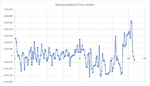
Figure 3. Deseasonlised time-series, xs, of the consumption shown in Figure 2; each point is the result of a subtraction between the current month and the same month of last year
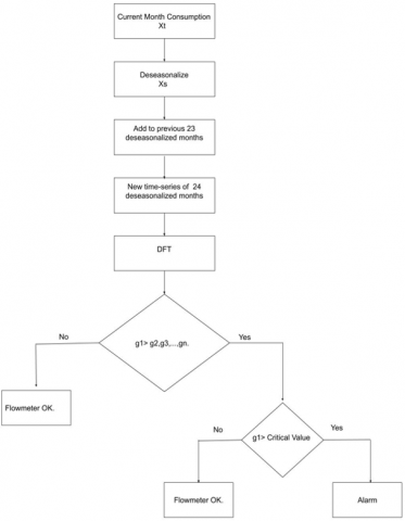
Figure 4. The detection scheme
In late April 2005, it was discovered that the flowmeter understudy was giving inaccurate readings when the flow recorded was inconsistent with the pressure recorded. What helped make this error in measurement go unchecked for many years is that the refinery owners informed the owners of the cooling-pumping station that they were going to take measures to reduce the cooling-water consumption to save costs. Later, the recorded flowmeter readings showed decreased consumption that was assumed to happen due to the water-saving actions taken by the refinery owners. At that time, it was also discovered that the decrease in the recorded cooling water was a result of a drifting flowmeter rather than any saving measures taken by the refinery, as explained in Ben Salamah et al. [11].
A detection scheme was designed to prevent this drift from reoccurring. This scheme depended on a particular property of a periodogram: drift is a trend. In a periodogram, a trend would appear at the first ordinate, R1. Consequently, the amplitude of the first ordinate would increase.
This scheme would take the deseasonalized time series, xs, resulting from Eq. (2) (shown in Figure 3) and transform it using the discrete Fourier Transform. Then, the g-statistic would be calculated and observed every month. It is assumed that if drift takes place, the g-statistic for the first ordinate would have the largest amplitude, and it will reach a critical value.
In more detail, the scheme would take the current, deseasonalized month and add it as the last datum to the previous 23 deseasonalized months, making a time series of 24 data. Then, this time series would be processed by the discrete Fourier transform (DFT) to produce twelve ordinates. Afterward, the g-statistic for every ordinate would be calculated and plotted. It is assumed that if a drift takes place, the amplitude of the first ordinate would be higher than the rest of the ordinates, and its g-statistic, g1, would reach or exceed the critical value of 0.400822 in Fisher's test of significance. The scheme is shown in Figure 4. To produce the discrete Fourier transform (DFT), NumXL was used. NumXL is an M.S. Excel Add-in.
It works as follows. First, the current month's consumption is taken. Second, the reading is deseasonalized by subtracting it from the same month of the previous year. Third, the deseasonalized consumption is added to the last 23 deseasonalized consumptions. Fourth, a new time series of 24 deseasonalized consumptions is formed. Fifth, the discrete Fourier transform (DFT) is applied over the previously mentioned time series to produce twelve ordinates. Sixth, the g-statistic of every ordinate is calculated and plotted. Sixth, a test would be applied to see if g1 is greater than g2,g3,..., g12. If g1 is not greater than g2,g3,..., g12, it is concluded that the flowmeter is not drifting. On the other hand, if g1 is greater than g2,g3,..., g12, a further test would be applied. This test examines the value of g1. If g1 is less than the critical value of 0.400822, the flowmeter would be considered functioning without drift. In contrast, if g1 is greater than the critical value of 0.400822, an alarm would indicate that the flowmeter might be drifting
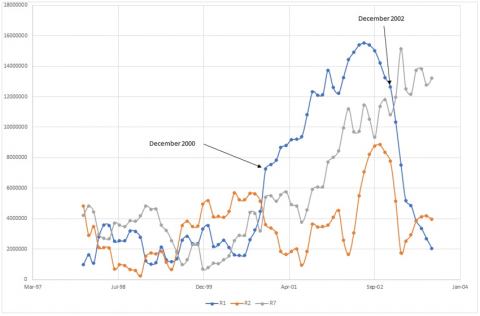
The ordinates (R's) are plotted against time in Figure 5. An enlarged view having only three ordinates (R1, R2, and R7) is shown in Figure 6.
As expected, the first ordinate, R1, representing the drift or trend component, became having the highest amplitude of all ordinates from December 2000 until December 2002. This phenomenon might indicate that the drift started in December 2000 and continued until it was discovered in April 2005. The fact that the first ordinate, R1, reduced in amplitude after 2002 can be explained by too much erroneous data entering the detection scheme to the extent that it was corrupted.
The Fisher statistic for the g-statistic of the first ordinate, g1, is plotted in Figure 7. The highest value that the Fisher statistic for the first ordinate, g1, has reached was 0.278. This value is less than the critical value of 0.400822.
Figure 5. The twelve ordinates of the time series over time
Figure 6. R1, R2, and R7 over time
Figure 7. The Fisher statistic for the first ordinate, g1, over time
Using the discrete Fourier transform to detect flowmeter drift by observing the increasing amplitude of the first ordinate succeeded. The previous detection scheme (using CUSUM) of Ben Salamah et al. [11] was able to detect drift in December 2001. The current detection scheme was able to catch the same drift a year earlier, in December 2000. This improvement is a considerable improvement.
Nevertheless, g1, the g-statistic of the first ordinate, has not reached the critical value of 0.400822 by Fisher's test of significance. Three possible causes could explain this result:
(1) The first ordinate reached a significant value. Nevertheless, this value was not detectable by Fisher's test.
(2) The Fisher test is unnecessary, and what is sufficient is that the first ordinate exceeds the rest of the ordinates.
(3) Other measures should have been made with the data.
Regarding the first possible reason, it has been known for a long time that Fisher's test could reject ordinate peaks that are important. In other words, Fisher's test is capable of deeming significant values as insignificant. Shimshoni [21] referred to the test as "perhaps too severe." To explain his point, Shimshoni wrote "Nowroozi (1965, 1966), in analysing the Alaskan and Rat Island earthquakes, applied a test developed by Fisher (1929). In a later study, Nowroozi (1967) described his use of Fisher's test and furthermore published tables to be used with that test. In applying Nowroozi's ideas to some actual records, Jarosch (1970 private communication) found that several amplitudes which seemed meaningful to him were rejected by a 95 per cent significance test suggested by Nowroozi. Nowroozi himself, in his 1965 and 1966 studies, labelled some periods as plausible although his significance test rejected them. It thus seemed that the test was perhaps too severe."
Russel [22] also commented on Fisher's test that "This test could be regarded as ultra-conservative." There are alternates to Fisher's test that include Siegel [23], who proposed a one-parameter family of tests that contains Fisher's test as a special case.
The second possible reason is that Fisher's test is unnecessary (in this case) to detect flowmeter drift, and observing the amplitude of the first ordinate, R1, only is enough. If the first ordinate (which indicates the existence of a trend) becomes more substantial than the rest of the ordinates, this is enough evidence for the possible presence of drift.
The last possible reason states that the numbers produced from the data should have been processed differently. One possible approach is the use of 'data windows' in the process of drift detection. For more information on data windows, the reader is referred to Warner [15], Bloomfield [16], and Lyons [24].
The investigation of the above-mentioned possible causes could be the subject of future work.
One severe limitation of the current detection scheme is its dependence on monthly consumption. Each datum requires one month to be produced. The detection scheme employed needs 24 pieces of data to conduct the analysis, an equivalent of two years. As a result, the scheme is inapplicable to new plants. Finding ways to lessen the period required before starting the analysis could be the subject of future studies.
Also, while the detection scheme using DFT could detect drift one year earlier than the one using CUSUM, there is a legitimate concern that this achievement might be attributed to using more data rather than the method itself. Comparing the performance of the two schemes over the same data could be the subject of a future study.
A flowmeter detection scheme was designed and presented to detect drifts by using the discrete Fourier transform. The detection scheme observed the behavior of the first ordinate, R1. If the amplitude of the first ordinate, R1, was higher than the rest of the ordinates, it might indicate that drift is taking place. Fisher's significance test determines the significance of the peak formed by an ordinate. Drift did occur, and, as expected, the magnitude of the first ordinate became the highest ordinate for a long time. However, this increase in magnitude was not deemed significant by Fisher's test. Further investigation is needed to determine the cause of this.
The authors would like to express their gratitude to the reviewer of this paper for his valuable suggestions. Kuwait's Public Authority for Applied Education and Training funded this research. It was done when the first author was on sabbatical leave from the Higher Institute for Energy (part of the Public Authority for Applied Education and Training). The sabbatical leave was spent in the Industrial & Management Systems Engineering Department of Kuwait University.
|
d |
period of the sinusoidal time series |
|
g |
Fisher test of significance (known as the g statistic) |
|
R |
the amplitude of the sinusoidal time-series. |
|
Rp |
periodogram ordinates at the Fourier frequencies |
|
t |
the order of observation with respect to time |
|
xs |
transformed datum |
|
xt |
original datum at time t |
|
xt-d |
original datum at time t-d |
|
µ |
the mean of the sinusoidal time-series |
|
$\Phi$ |
the phase of the sinusoidal time-series |
[1] Ben Salamah, M. (2010). Design and Support of Systems for Operation and Maintenance of a Cooling Petrochemical Pumping Station. Doctoral dissertation, Swinburne University of Technology, Melbourne, Australia.
[2] Hayward, A.T. (1979). Flowmeters: A Basic Guide and Source-Book for Users. Macmillan International Higher Education.
[3] Leonard, D. (2009). The ignored negative impacts of downsizing. Journal for Quality and Participation, 32(2): 1-3.
[4] Bisgaard, S.R., Kulahci, M. (2007). Quality Quandaries: Practical time series modeling. Quality Engineering, 19(3): 253-262. https://doi.org/10.1080/08982110701577837
[5] Bisgaard, S.R., Kulahci, M. (2007). Quality Quandaries practical time series modeling II. Quality Engineering, 19(4): 393-400. https://doi.org/10.1080/08982110701456560
[6] Bisgaard, S.R., Kulahci, M. (2008). Quality Quandaries: Forecasting with seasonal time series models. Quality Engineering, 20(2): 250-260. https://doi.org/10.1080/08982110801924624
[7] Bisgaard, S., Kulahci, M. (2009). Quality Quandaries*: Time series model selection and parsimony. Quality Engineering, 21(3): 341-353. https://doi.org/10.1080/08982110903025197
[8] Bowerman, B.L., O'Connell, R.T. (1979). Time Series and Forecasting. North Scituate, MA: Duxbury Press.
[9] Technical Glossary for sensors and instrumentation | OMEGA. [Online]. Available: https://www.omega.co.uk/techref/glossary.html#d, accessed: 04-Mar-2020.
[10] Morris, A.S., Langari, R. (2012). Measurement and Instrumentation: Theory and application. Academic Press.
[11] Ben Salamah, M., Kapoor, A., Savsar, M., Ektesabi, M., Abdekhodaee, A., Shayan, E. (2011). The detection of flow meter drift by using statistical process control. International Journal of Sustainable Development and Planning, 6(1): 91-103. https://doi.org/10.2495/SDP-V6-N1-91-103
[12] Ben Salamah, M., Palaneeswaran, E., Savsar, M., Ektesabi, M. (2011). Detecting flow meter drift by using artificial neural networks. International Journal of Sustainable Development and Planning, 6(4): 512-521. https://doi.org/10.2495/SDP-V6-N4-512-521
[13] Transnational College of Lex. (2012). Who Is Fourier? A Mathematical Adventure 2nd Edition, Second Edition. Cambridge, Mass: Language Research Foundation.
[14] Kaplan, H.L. (1983). Correlations, contrasts, and components: Fourier analysis in a more familiar terminology. Behavior Research Methods & Instrumentation, 15(2): 228-241. https://doi.org/10.3758/BF03203554
[15] Warner, R.M. (1998). Spectral Analysis of Time-Series Data. Guilford Press.
[16] Bloomfield, P. (2004). Fourier Analysis of Time Series: An Introduction. John Wiley & Sons.
[17] Fisher, R.A. (1929). Tests of significance in harmonic analysis. Proceedings of the Royal Society of London. Series A, Containing Papers of a Mathematical and Physical Character, 125(796): 54-59. https://doi.org/10.1098/rspa.1929.0151
[18] Nowroozi, A.A. (1967). Table for Fisher's test of significance in harmonic analysis. Geophysical Journal International, 12(5): 517-520. https://doi.org/10.1111/j.1365-246X.1967.tb03132.x
[19] Al-Khafaji, A.W., Tooley, J.R. (1986). Numerical Methods in Engineering Practice, p. 190. New York: Holt, Rinehart and Winston.
[20] AJ Design Software. Linear Interpolation Equation Calculator Engineering - Interpolator Formula. [Online]. Available: https://www.ajdesigner.com/phpinterpolation/linear_interpolation_equation.php, accessed: 08-Mar-2020.
[21] Shimshoni, M. (1971). On Fisher's test of significance in harmonic analysis. Geophysical Journal International, 23(4): 373-377. https://doi.org/10.1111/j.1365-246X.1971.tb01829.x
[22] Russell, R.J. (1985). Significance tables for the results of Fast Fourier Transforms. British Journal of Mathematical and Statistical Psychology, 38(1): 116-119. https://doi.org/10.1111/j.2044-8317.1985.tb00820.x
[23] Siegel, A.F. (1980). Testing for periodicity in a time series. Journal of the American Statistical Association, 75(370): 345-348. https://doi.org/10.1080/01621459.1980.10477474
[24] Lyons, R.G. (2004). Understanding Digital Signal Processing, 3/E. Pearson Education India.