Iman I. Gorial
© 2021 IIETA. This article is published by IIETA and is licensed under the CC BY 4.0 license (http://creativecommons.org/licenses/by/4.0/).
OPEN ACCESS
The aims of this paper are to propose approach of explicit finite difference mathod (EFDM), clarify the problem the mixed fractional derivative in one-dimensional fractional percolation equation (O-DFPE), and the study of consistency, stability, and convergence methods. Use of estimated Grunwald estimation in the analysis of mixed fractional derivatives. However, the given method is successfully applied to the mixed fractional derivative classes with the initial condition (IC) and derivative boundary conditions (DBC). To illustrate the efficiency and validity of the proposed algorithm, examples are given and the results are compared with the exact solution. From the figures shown for the examples in this work, the approximate solution values given by the EFDM for the various grid points are equivalent to the exact solution values with high-precision approximation. To show the effectiveness of the proposed method, where the error between the EFDM and the exact method is zero, the fractional derivative was used with various and random values. Using the package MATLAB and MathCAD 12 Figures were introduced.
fractional derivative, explicit finite difference method (EFDM), fractional percolation equation (FPE), stability, convergence of numerical method
Seepage hydraulics, groundwater hydraulics, groundwater dynamics, and fluid dynamics in porous media are all modeled using fractional percolation equations (FPEs), which are derived from classical integer order percolation equations [1-6]. Under the hypotheses of continuity and Darcy's law, the regular integer percolation equation for incompressible, single phase percolation flow can be written as:
$\frac{1}{v} \frac{\partial \Theta(\varsigma, \mathcal{W})}{\partial \mathcal{W}}=\frac{\partial}{\partial \varsigma}\left(M(\varsigma) \frac{\partial \Theta(\varsigma, \mathcal{W})}{\partial \varsigma}\right)+f(\varsigma, \mathcal{W}), \varsigma \in \Omega$
where the percolation coefficient is $M(\varsigma)=M_{\varsigma}$, the pressure is $\Theta=\Theta(\varsigma, \mathcal{W}), v$ is the velocity, $f(\varsigma, \mathcal{W})$ is the source term. To deal with seepage flow movement in a non-homogeneous porous medium, He [7] first considered a modification of Darcy's law. It's possible to write it as
$\frac{1}{v} \frac{\partial \Theta}{\partial \mathcal{W}}=\frac{\partial^{\beta}}{\partial \varsigma^{\beta}}\left(M_{\varsigma} \frac{\partial^{\alpha} \Theta}{\partial \varsigma^{\alpha}}\right)+f(\varsigma, \mathcal{W}), \varsigma \in \Omega$
This equation is called the FPE equation.
where $0 \leq \beta \leq 1,0<\alpha<1$, and $q=M(\varsigma) \frac{\partial \Theta(\varsigma, W)}{\partial \varsigma}$ is the rate of mass flux in a fluid.
The Riemann-Liouville fractional derivative is the fractional derivative described above [8, 9].
The Riemann-Liouville fractional derivative $\frac{\partial \gamma{\Theta}(\varsigma, \mathcal{W})}{\partial \varsigma^{\gamma}}$ of the order is defined by:
$\frac{\partial^{\gamma} \Theta(\varsigma, \mathcal{W})}{\partial \varsigma^{\gamma}}=\frac{1}{\Gamma(n-\gamma)} \frac{\partial^{\gamma}}{\partial \varsigma^{\gamma}} \int_{0}^{\varsigma} \Theta(\varsigma, \mathcal{W})(\varsigma-s)^{-\gamma+n-1} d s$
where, $\gamma>0$, and $n-1<\gamma \leq n$. If $\beta=0$, then the FPE can be represented as:
$\frac{1}{v} \frac{\partial \Theta}{\partial \mathcal{W}}=\frac{\partial^{0}}{\partial \varsigma^{0}}\left(M_{\varsigma} \frac{\partial^{\alpha} \Theta}{\partial \varsigma^{\alpha}}\right)+f(\varsigma, \mathcal{W}), \varsigma \in \Omega$
This paper will be interested with the expansion of EFDM where the emphasis would be on a particular type of v=1 and initial- derivative boundary conditions of O-DFPE which discuss unknown pressure function $\Theta(\varsigma, \mathcal{W})$ satisfying:
$\frac{\partial \Theta}{\partial \mathcal{W}}=\frac{\partial^{\beta}}{\partial \varsigma^{\beta}}\left(M_{\varsigma} \frac{\partial^{\alpha} \Theta}{\partial \varsigma^{\alpha}}\right)+f(\varsigma, \mathcal{W})$ (1)
the initial condition (IC) with derivative boundary conditions (DBC):
$\Theta(\varsigma, 0)=\varphi(\varsigma)$
$\Theta_{\varsigma}(0, \mathcal{W})=\pi_{1}(\mathcal{W}), 0<\mathcal{W} \leq T$ (2)
$\Theta_{\zeta}(1, \mathcal{W})=\pi_{2}(\mathcal{W}), 0<\mathcal{W} \leq T$
where, $0 \leq \beta \leq 1,0<\alpha<1$ and the pressure is $\Theta=\Theta(\varsigma, \mathcal{W})$. The percolation coefficient is $M(\varsigma)=M_{\varsigma}, \pi_{1}, \pi_{2}$ are known function of $\omega. f(\varsigma, \mathcal{W})$ is the source term. The $\alpha, \beta$ is fractional derivative order shifted Grunwald estimate are defined as:
$\frac{\partial^{\alpha} \Theta(\varsigma, \mathcal{W})}{\partial \varsigma^{\alpha}}=\frac{1}{(\Delta \varsigma)^{\alpha}} \sum_{p=0}^{i+1} g_{\alpha, p} \Theta_{i-p+1}^{s}+\mathrm{O}(\Delta \varsigma)$
The numerical solutions are examined in this paper of the equation for fractional percolation. Paper structure is as follows. Section 2, we present Literature review. In Section 3, the EFDM for solving O-DFPE is proposed. In Section 4, its convergence is discussed of the EFDM. In Section 5, numerical simulation and comparison are provided to assess the method 's efficiency.
Since most fractional differential equations do not have explicit analytic solutions, many authors rely on numerical solution strategies based on convergence and stability analysis. [10-18]
Recently, Liu et al. [19] considered numerical simulation with porous media fractional derivatives for the 3D seepage flow. For the one-dimensional FPE, Chen et al. [20] developed a novel implicit finite difference process. For the two-dimensional case of FPE, Chen et al. [21] considered an alternating direction implicit difference procedure. The numerical simulation of variable-order fractional percolation equation in non-homogenous porous media was discussed by Chen et al. [22]. For the two-dimensional FPE, A second order finite difference method was suggested by Guo et al. [23].
In this work we look at the EFDM where will concentrate on a class of v=1 and IC with DBC of O-DFPE.
We define EFDM for Eq. (1), and it can be rewritten as the following form:
$\frac{\partial \Theta}{\partial \mathcal{W}}=\frac{\partial^{\beta} M_{\varsigma}}{\partial \varsigma^{\beta}}\left(\frac{\partial^{\alpha} \Theta}{\partial \varsigma^{\alpha}}\right)+M_{\varsigma}\left(\frac{\partial^{\alpha+\beta} \Theta}{\partial \varsigma^{\alpha+\beta}}\right)+f(\varsigma, \mathcal{W})$ (3)
First, we create a computational uniform grid for the derivation of the EFDM for O-DFPE with variable coefficients by $\varsigma_{i}=a+i \Delta \varsigma$, where $\Delta \varsigma=(\mathrm{b}-\mathfrak{a}) / \mathrm{n}$ for $\mathrm{i}=0, \ldots, \mathrm{n}$ and $\mathcal{W}_{\mathrm{s}}=\mathrm{s} \Delta \mathcal{W}$, where $\Delta \mathcal{W}=T / M$ for $\mathfrak{s}=0, \ldots, M .$ And $0 \leq$$\beta \leq 1,0<\alpha<1$
And using Eq. (2) with applied the forward Euler:
$\left.\frac{\partial \Theta}{\partial \mathcal{W}}\right|_{\left(\varsigma_{i}, w_{s}\right)} \sim \frac{\Theta\left(\varsigma_{i}, \mathcal{W}_{s+1}\right)-\Theta\left(\varsigma_{i}, \mathcal{W}_{s}\right)}{\Delta \mathcal{W}}+\mathrm{o}(\Delta \mathcal{W})$
Moreover, it is possible to define the mixed fractional derivatives used in Eq. (3):
$\left.\frac{\partial^{\beta} M_{\varsigma}}{\partial \varsigma^{\beta}}\left(\frac{\partial^{\alpha} \Theta}{\partial \varsigma^{\alpha}}\right)\right|_{\left(\varsigma_{i}, w_{s}\right)}+\left.M_{\varsigma}\left(\frac{\partial^{\beta+\alpha} \Theta}{\partial \varsigma^{\beta+\alpha}}\right)\right|_{\left(\varsigma_{i}, w_{s}\right)}$$={\mathrm{M}}_{\varsigma}^{\prime}\left(\frac{1}{\Delta \varsigma^{\alpha}} \sum_{p=0}^{i+1} g_{\alpha, p} \Theta_{i-p+1}^{s}\right)+\frac{M_{\varsigma}}{\Delta \varsigma^{\beta+\alpha}} \sum_{p=0}^{i+1} g_{\beta+\alpha, p} \Theta_{i-p+1}^{s}$
Now we use explicit Euler method to even get $\Theta_{i}^{S+1}$:
$\frac{\Theta_{i}^{s+1}-\Theta_{i}^{s}}{\Delta \mathcal{W}}=\hat{\mathrm{M}}_{\varsigma}^{\prime}\left(\frac{1}{\Delta \varsigma^{\alpha}} \sum_{p=0}^{i+1} g_{\alpha, p} \Theta_{i-p+1}^{s}\right)+M_{\varsigma}\left(\frac{1}{\Delta \varsigma^{\beta+\alpha}} \sum_{p=0}^{i+1} g_{\beta+\alpha, p} \Theta_{i-p+1}^{s}\right)+f_{i}^{s}$
$\Theta_{i}^{s+1}=\mathrm{M}_{\varsigma}^{\prime}\left(\frac{\Delta \mathcal{W}}{\Delta \varsigma^{\alpha}} \sum_{p=0}^{i+1} g_{\alpha, p} \Theta_{i-p+1}^{s}\right)+M_{\varsigma}\left(\frac{\Delta \mathcal{W}}{\Delta \varsigma^{\beta+\alpha}} \sum_{p=0}^{i+1} g_{\beta+\alpha, p} \Theta_{i-p+1}^{s}\right)+\Theta_{i}^{s}+\Delta \mathcal{W} f_{i}^{S}$ (4)
where:
$g_{\alpha, r}=(-1)^{r} \frac{\alpha(\alpha-1) \cdots(\alpha-r+1)}{r !}$
$g_{\beta+\alpha, r}=(-1)^{r} \frac{(\beta+\alpha)(\beta+\alpha-1) \cdots(\beta+\alpha-r+1)}{r !}, \mathrm{r}=0,1,2, \ldots$ (5)
To prove the convergence of the proposed method, we will need proof of conditionally stable and consistent according to the equivalence theorem of Lax.
4.1 Stability of EFDM
Now, we must prove that O-DFPE by EFDM is conditionally stable:
Theorem: The Eq. (4) with $0 \leq \beta \leq 1,0<\alpha<1$ is conditionally stable if
$\frac{\alpha \mathrm{M}_{\varsigma \max }^{\prime} \Delta \mathcal{W}}{\Delta \varsigma^{\alpha}} \leq 1+\frac{\beta \mathrm{M}_{\varsigma_{\max }} \Delta \mathcal{W}}{\Delta \varsigma^{\beta+\alpha}}+\frac{\alpha \mathrm{M}_{\varsigma_{\max }} \Delta \mathcal{W}}{\Delta{ }^{\beta+\alpha}}$
Proof:
The equations system defined by (4) can be written in the form of $\underline{\Theta^{S+1}}=\underline{\varrho \Theta^{S}}+\Delta \mathcal{W} \underline{Q^{s}}$ where
$\underline{\Theta^{s+1}}=\left[\Theta_{1}^{s+1}, \Theta_{2}^{s+1}, \ldots, \Theta_{n-1}^{s+1}\right]^{T}$
$\Delta \mathcal{W} \underline{F^{s}}=\left[\Delta \mathcal{W} f_{1}^{s}, \Delta \mathcal{W} f_{2}^{s}, \ldots, \Delta \mathcal{W} f_{n-1}^{s}\right]^{T}$
and
$\varrho_{i, j}=\left\{\begin{array}{cc}1+\mu_{i} g_{\alpha, 1}+\mathrm{N}_{i} g_{\beta+\alpha, 1} & \text { for } \quad j=i \\ \mu_{i} g_{\alpha, 0}+\mathrm{N}_{i} g_{\beta+\alpha, 0} & \text { for } j=i-1 \\ \mu_{i} g_{\alpha, 2}+\mathrm{N}_{i} g_{\beta+\alpha, 2} & \text { for } j=i+1 \\ \mu_{i} g_{\alpha, j+1}+\mathrm{N}_{i} g_{\beta+\alpha, j+1} & \text { for } j<i+1\end{array}\right.$
matrix entries are $\underline{\varrho_{i, j}}$ for $i=1,2, \ldots, n-1$ and $j=1, \ldots, n-1$.
where the coefficients
$\mu_{i}=\frac{{\mathrm{M}}_{\varsigma}^{\prime} \Delta \mathcal{W}}{\Delta \varsigma^{\alpha}} \quad$ and $\quad \mathrm{N}_{i}=\frac{\mathrm{M}_{\varsigma} \Delta \mathcal{W}}{\Delta \varsigma^{\beta+\alpha}}$
To get to:
$\begin{aligned} \Theta_{1}^{s+1}=\left(\mu_{1} g_{\alpha, 0}+\right.& \left.\mathrm{N}_{1} g_{\beta+\alpha, 0}\right) \Theta_{0}^{s} \\ &+\left(1+\mu_{1} g_{\alpha, 1}+\mathrm{N}_{1} g_{\beta+\alpha, 1}\right) \Theta_{1}^{s} \\ &+\left(\mu_{1} g_{\alpha, 2}+\mathrm{N}_{1} g_{\beta+\alpha, 2}\right) \Theta_{2}^{s}+\cdots \\ &+\left(\mu_{1} g_{\alpha, n}+\mathrm{N}_{1} g_{\beta+\alpha, n}\right) \Theta_{n}^{s} \\ &+\Delta \mathcal{W} f_{1}^{s} \end{aligned}$
$\begin{aligned} \Theta_{2}^{s+1}=\left(\mu_{2} g_{\alpha, 0}+\right.& \left.\mathrm{N}_{2} g_{\beta+\alpha, 0}\right) \Theta_{0}^{s} \\ &+\left(1+\mu_{2} g_{\alpha, 1}+\mathrm{N}_{2} g_{\beta+\alpha, 1}\right) \Theta_{1}^{s} \\ &+\left(\mu_{2} g_{\alpha, 2}+\mathrm{N}_{2} g_{\beta+\alpha, 2}\right) \Theta_{2}^{S} \\ &+\left(\mu_{2} g_{\alpha, 3}+\mathrm{N}_{2} g_{\beta+\alpha, 3}\right) \Theta_{3}^{s}+\cdots \\ &+\left(\mu_{2} g_{\alpha, n}+\mathrm{N}_{2} g_{\beta+\alpha, n}\right) \Theta_{n}^{s} \\ &+\Delta \mathcal{W} f_{2}^{s} . \end{aligned}$
$\Theta_{n-1}^{s+1}=\left(\mu_{n-1} g_{\alpha, 0}+\mathrm{N}_{n-1} g_{\beta+\alpha, 0}\right) \Theta_{0}^{s / 3}$
$+\left(1+\mu_{n-1} g_{\alpha, 1}\right.$$\left.\quad+\mathrm{N}_{n-1} g_{\beta+\alpha, 1}\right) \Theta_{1}^{s}$
$+\left(\mu_{n-1} g_{\alpha, 2}+\mathrm{N}_{n-1} g_{\beta+\alpha, 2}\right) \Theta_{2}^{s}$$+\cdots$
$+\left(\mu_{n-1} g_{\alpha, n}+\mathrm{N}_{n-1} g_{\beta+\alpha, n}\right) \Theta_{n}^{s / 3}$$+\Delta \mathcal{W} f_{n-1}^{s}$
According to the Greshgorin theorem [24],
$\varrho_{i, j}=1+\left(\frac{\mathrm{M}_{\varsigma}^{\prime} \Delta \mathcal{W}}{\Delta \varsigma^{\alpha}} g_{\alpha, 1}+\frac{\beta \mathrm{M}_{\varsigma} \Delta \mathcal{W}}{\Delta \varsigma^{\beta+\alpha}} g_{\beta+\alpha, 1}\right)$
$=1-\frac{\alpha \mathrm{M}_{\varsigma}^{\prime} \Delta \mathcal{W}}{\Delta \varsigma^{\alpha}}-\frac{\beta \mathrm{M}_{\varsigma} \Delta \mathcal{W}}{\Delta \varsigma^{\beta+\alpha}}-\frac{\alpha \mathrm{M}_{\varsigma} \Delta \mathcal{W}}{\Delta \varsigma^{\beta+\alpha}}$
and
$\begin{aligned} \vartheta_{i}=\sum_{l=0}^{n} & \varrho_{i, l}=\frac{{\mathrm{M}}_{\varsigma}^{\prime} \Delta \mathcal{W}}{\Delta \varsigma^{\alpha}} \sum_{l=0}^{n} g_{\alpha, i-j+1} \\ &+\frac{\mathrm{M}_{\varsigma} \Delta \mathcal{W}}{\Delta \varsigma^{\beta+\alpha}} \sum_{l=0}^{n} g_{\beta+\alpha, i-j+1} \\ & \leq \frac{\alpha {\mathrm{M}}_{\varsigma}^{\prime} \Delta \mathcal{W}}{\Delta \varsigma^{\alpha}}+\frac{\beta \mathrm{M}_{\varsigma} \Delta \mathcal{W}}{\Delta \varsigma^{\beta+\alpha}}+\frac{\alpha \mathrm{M}_{\varsigma} \Delta \mathcal{W}}{\Delta \varsigma^{\beta+\alpha}} \end{aligned}$
Now
$\vartheta_{i}=\sum_{l=0}^{n} \varrho_{i, l}$.
and therefore $\varrho_{i, j}+\vartheta_{i} \leq 1$. we also have
$\varrho_{i, j}-\vartheta_{i} \geq\left(1-\frac{\alpha {\mathrm{M}}_{\varsigma}^{\prime} \Delta \mathcal{W}}{\Delta \varsigma^{\alpha}}-\frac{\beta \mathrm{M}_{\varsigma} \Delta \mathcal{W}}{\Delta \varsigma^{\beta+\alpha}}-\frac{\alpha \mathrm{M}_{\varsigma} \Delta \mathcal{W}}{\Delta \varsigma^{\beta+\alpha}}\right)-\left(\frac{\alpha {\mathrm{M}}_{\varsigma}^{\prime} \Delta \mathcal{W}}{\Delta \varsigma^{\alpha}}+\frac{\beta \mathrm{M}_{\varsigma} \Delta \mathcal{W}}{\Delta \varsigma^{\beta+\alpha}}+\frac{\alpha \mathrm{M}_{\varsigma} \Delta 2 \mathcal{W}}{\Delta \varsigma^{\beta+\alpha}}\right)$
$=1-\frac{2 \alpha {\mathrm{M}}_{\varsigma}^{\prime} \Delta \omega}{\Delta \varsigma^{\alpha}}-\frac{2 \beta \mathrm{M}_{\varsigma} \Delta \omega}{\Delta \varsigma^{\beta+\alpha}}-\frac{2 \alpha \mathrm{M}_{\varsigma} \Delta \omega}{\Delta \varsigma^{\beta+\alpha}}$
$\geq 1-\frac{2 \alpha \mathrm{M}_{\varsigma \max }^{\prime} \Delta \mathcal{W}}{\Delta \varsigma^{\alpha}}-\frac{2 \beta \mathrm{M}_{\varsigma \max } \Delta \mathcal{W}}{\Delta \varsigma^{\beta+\alpha}}-\frac{2 \alpha \mathrm{M}_{\varsigma \max } \Delta \mathcal{W}}{\Delta \varsigma^{\beta+\alpha}}$
Then:
$1-\frac{2 \alpha \mathrm{M}_{\varsigma \max }^{\prime} \Delta \mathcal{W}}{\Delta \varsigma^{\alpha}}-\frac{2 \beta \mathrm{M}_{\varsigma \max } \Delta \mathcal{W}}{\Delta \varsigma^{\beta+\alpha}}-\frac{2 \alpha \mathrm{M}_{\varsigma \max } \Delta \mathcal{W}}{\Delta \varsigma^{\beta+\alpha}} \geq-1$
$\rightarrow-1+\frac{2 \alpha \mathrm{M}_{\varsigma_{\max }}^{\prime} \Delta \mathcal{W}}{\Delta \varsigma^{\alpha}}+\frac{2 \beta \mathrm{M}_{\varsigma \max } \Delta \mathcal{W}}{\Delta \varsigma^{\beta+\alpha}}+\frac{2 \alpha \mathrm{M}_{\varsigma \max } \Delta \mathcal{W}}{\Delta \varsigma^{\beta+\alpha}} \leq 1$
$\rightarrow \frac{\alpha \mathrm{M}_{\varsigma_{\max }}^{\prime} \Delta \mathcal{W}}{\Delta \varsigma^{\alpha}} \leq 1+\frac{\beta \mathrm{M}_{\varsigma \max } \Delta \mathcal{W}}{\Delta \varsigma^{\beta+\alpha}}+\frac{\alpha \mathrm{M}_{\varsigma \max } \Delta \mathcal{W}}{\Delta \varsigma^{\beta+\alpha}}$
4.2 Consistency of EFDM
Notice that the time difference operator in (4) has a local truncation error of order $\mathrm{O}(\Delta \omega)$ and the space difference operators in (4) have local truncation errors of orders $\mathrm{O}(\Delta \varsigma)$. Similar to Lemma 2.1 in in [11], we can obtain the the consistency of the O-DFPE is:
$\mathrm{O}(\Delta \varsigma)+\mathrm{O}(\Delta \mathcal{W})$
Now we can apply the Laxs equivalence theorem [25] after we obtain consistency and conditionally stable. Where it converges at the rate of $\mathrm{O}(\Delta \varsigma+\Delta \mathcal{W})$.
Some numerical results are discussed in this section to help our theoretical analysis to illustrate the efficacy of method use.
Example 1: Consider the following O-DFPE:
$\frac{\partial \Theta}{\partial \mathcal{W}}=5.3 \varsigma^{0.5} e^{-w}-\varsigma^{2} e^{-w}-6.8 \varsigma^{0.5} e^{-w}$
$+\frac{\partial}{\partial \varsigma}\left(\left(30-\varsigma^{2}\right) \frac{\partial^{0.5} \Theta}{\partial \varsigma^{0.5}}\right)$
Subjects to the IC and DBC:
$\Theta(\varsigma, 0)=\varsigma^{2}$
$\Theta_{\varsigma}(0, \mathcal{W})=0, \quad 0<\mathcal{W} \leq T$
$\Theta_{\varsigma}(1, \mathcal{W})=2 e^{-W}, \quad 0<\mathcal{W} \leq T$
That the EXS to this problem is:
$\Theta(\varsigma, \mathcal{W})=e^{-W} v_{\varsigma^{2}}$
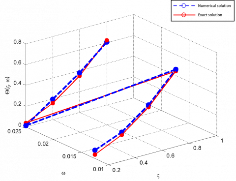
Figure 1 indicates the solution obtained using EFDM versus the exact solution at $\varsigma=0.2,0.4,0.6,0.8,1$ and $\Delta \mathcal{W}=0.0125$ when $\beta=1, \alpha=0.5$. Figure 1 clearly demonstrates that EFDM's numerical solutions are excellent and consistent with exact solutions, illustrating the utility of the proposed zero-error method.
Figure 1. The numerical solution and EXS of example 1
Example 2: Consider the following O-DFPE:
$\frac{\partial \Theta}{\partial \mathcal{W}}=-\left(\varsigma^{2}+2.3 \varsigma^{0.3}\right) e^{-w}+\frac{\partial^{0.9}}{\partial \varsigma^{0.9}}\left(\frac{\partial^{0.8} {\Theta}}{\partial \varsigma^{0.8}}\right)$
Subjects to the IC and DBC:
$\Theta( \varsigma, 0)= \varsigma^{2}$
$\Theta_{\varsigma}(0, \mathcal{W})=0,0<\mathcal{W} \leq T$
$\Theta_{\varsigma}(1, \mathcal{W})=2 e^{-w}, 0<\mathcal{W} \leq T$
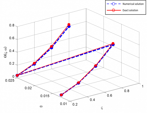
Figure 2. The numerical solution and EXS of example 2
That the EXS to this problem is: $\Theta(\varsigma, \mathcal{W})=e^{-\mathcal{W}} \varsigma^{2}$
Shown in Figure 2 Comparison between exact solution and EFDM at $\varsigma=0.2,0.4,0.6,0.8,1$ and $\Delta \mathcal{W}=0.0125$ and when $\beta=0.9, \alpha=0.8$. Clearly shown that the numerical solution of EFDM is identical to the exact solution, indicating the efficacy of the proposed approach with a zero error rate.
Example 3: Consider the following O-DFPE:
$\frac{\partial \Theta}{\partial \mathcal{W}}=4.01 \varsigma^{2.5} e^{-w}-\varsigma^{2} e^{-w}-3.96 \varsigma^{0.5} e^{-w}$
$+\frac{\partial^{0.8}}{\partial \varsigma^{0.8}}\left(\left(-\varsigma^{2}+20\right) \frac{\partial^{0.7} \Theta}{\partial \varsigma^{0.7}}\right)$
$\varsigma \in \Omega, \mathcal{W}>0$
Subjects to the IC and DBC:
$\Theta(\varsigma, 0)=\varsigma^{2}$
$\Theta_{\varsigma}(0, \mathcal{W})=00<\mathcal{W} \leq T$
$\Theta_{\varsigma}(1, \mathcal{W})=2 e^{-w}, 0<\mathcal{W} \leq T$
That the EXS to this problem is: $\Theta(\varsigma, \mathcal{W})=e^{-\mathcal{W}}{ }_{\varsigma}^{2}$.
Figure 3 shows a comparison between the exact solution and the EFDM with $\varsigma=0.2,0.4,0.6,0.8,1$ and $\Delta \mathcal{W}=0.0125$ and $\beta=0.8, \alpha=0.7$ with an error equal to zero. Figure 3 clearly shows that the numerical solutions of EFDM are excellent and compatible with the exact solutions, demonstrating the usefulness of the proposed approach with zero error.
Figure 3. The numerical solution and EXS of example 3
Example 4: Consider the following O-DFPE:
$\frac{\partial \Theta}{\partial w}=\left(4.2 \varsigma^{2.5}+0.3 \varsigma^{0.5}+0.6 \varsigma^{-1.5}\right) e^{-W}+$
$\frac{\partial^{0.7}}{\partial \varsigma^{0.7}}\left(\left(-\varsigma^{2}+2\right) \frac{\partial^{0.8} \Theta}{\partial \varsigma^{0.8}}\right)-\left(\varsigma^{2}+1+4.4 \varsigma^{0.5}\right) e^{-W}$
$\varsigma \in \Omega, \mathcal{W}>0$
Subjects to the IC and DBC:
$\Theta(\varsigma, 0)=\varsigma^{2}$
$\Theta_{\varsigma}(0, \mathcal{W})=0, \quad 0<\mathcal{W} \leq T$
$\Theta_{\varsigma}(1, \mathcal{W})=2 e^{-\omega}, \quad 0<\mathcal{W} \leq T$
That the EXS to this problem is: $\Theta(\varsigma, \mathcal{W})=e^{-w} \varsigma^{2}$.
Figure 4 demonstrates the relation between the numerical solution of EFDM and the exact solution for the numerical scheme at $\varsigma=0.2,0.4,0.6,0.8,1$ and $\Delta \mathcal{W}=0.0125$ and when $\beta=0.7, \alpha=0.8$. The approach to the numerical solution of EFDM can be seen to be similar to the exact solution.
Figure 4. The numerical solution and EXS of example 4
To model percolation properties, the O-DFPE was introduced. We suggested EFDM with the IC and DBC in this paper. The EFDM's stability and convergence with convergence order $\mathrm{O}(\Delta \varsigma+\Delta \mathcal{W})$were demonstrated. Furthermore, the proposed method has been successfully extended to the solution of various O-DFPE with mixed fractional derivative groups. This algorithm is quick and straightforward to implement. We also proposed a numerical experiment to help the theoretical analysis and show the practicality of the number scheme in order to demonstrate the efficacy of EFDM. However, a comparison of exact and approximate solution values reveals that the approximate solution values obtained by EFDM are equivalent to the exact solution values obtained with high precision approximation for different grid points. It's also worth remembering that as the approximation order grows, the accuracy rises with it.
|
DBC |
Derivative boundary conditions |
|
EFDM |
Explicit finite difference method |
|
FPE |
Fractional percolation equation |
|
O-DFPE |
One-dimensional fractional percolation equation |
|
IC |
Initial condition |
|
T |
Constant |
|
Greek symbols |
|
|
$\underline{\varrho_{i, j}}$ |
Matrix entries |
|
$f(\varsigma, \mathcal{W})$ |
The source term |
|
$g_{\alpha, r}, g_{\beta+\alpha, r}$ |
The normalized Grunwald weights |
|
${M}_{\varsigma}^{\prime}$ |
Derivative of the percolation coefficient |
|
$M_{\varsigma}$ |
The percolation coefficient |
|
$\vartheta_{i}=\sum_{l=0}^{n} \varrho_{i, l}$ |
Radius |
|
$\Theta(\varsigma, \mathcal{W})$ |
Function of pressure |
|
$\Theta(\varsigma, 0)$ |
Initial condition |
|
$\Theta_{\varsigma}(0, \mathcal{W}), \Theta_{\varsigma}(1, \mathcal{W})$ |
Derivative boundary conditions |
|
$\alpha, \beta$ |
Derivatives in fractional order |
|
$\varphi(s)$ |
a well-known function $\varsigma$ |
|
$\pi_{1}(\mathcal{W}), \pi_{1}(\mathcal{W})$ |
a well-known function $\mathcal{W}$ |
[1] Chou, H., Lee, B., Chen, C. (2006). The transient infiltration process for seepage flow from cracks. Advances in Subsurface Flow and Transport: Eastern and Western Approaches III.
[2] Huang, A.X. (1996). A new decomposition for solving percolation equations in porous media. In Third International Symposium on Aerothermodynamics of Internal Flows, Beijing, China, 1: 417-420.
[3] Petford, N., Koenders, M.A. (2003). Seepage flow and consolidation in a deforming porous medium. Geophys. Res. Abstr., 5: 3329. https://www.researchgate.net/publication/241325258_Seepage_flow_and_consolidation_in_a_deforming_porous_medium.
[4] Thusyanthan, N.I., Madabhushi, S.P.G. (2003). Scaling of seepage flow velocity in centrifuge models. CUED/D-SOILS/TR326, pp. 1-13. https://doi.org/10.1016/0921-5093(93)90350-N
[5] Lin, R., Liu, F., Anh, V., Turner, I. (2004). Stability and convergence of a new explicit finite-difference approximation for the variable-order nonlinear fractional diffusion equation, Appl. Math. Comput., 212: 435-445. https://doi.org/10.1016/j.amc.2009.02.047
[6] Jia, J., Wang, H. (2015). Fast finite difference methods for space-fractional diffusion equations with fractional derivative boundary conditions. Journal of Computational Physics, 293: 359-369.
[7] He, J.H. (1998). Approximate analytical solution for seepage flow with fractional derivatives in porous media. Computer Methods in Applied Mechanics and Engineering, 167(1-2): 57-68. https://doi.org/10.1016/S0045-7825(98)00108-X
[8] Miller, K.S., Ross, B. (1993). An Introduction to the Fractional Calculus and Fractional Differential Equations. A Wiley-Interscience Publication.
[9] Podlubny, I. (1998). Fractional differential equations: an introduction to fractional derivatives, fractional differential equations, to methods of their solution and some of their applications. Elsevier. https://doi.org/10.1155/2013/802324
[10] Meerschaert, M.M., Tadjeran, C. (2004). Finite difference approximations for fractional advection-dispersion flow equations. Journal of Computational and Applied Mathematics, 172(1): 65-77. https://doi.org/10.1016/j.cam.2004.01.033
[11] Meerschaert, M.M., Scheffler, H.P., Tadjeran, C. (2006). Finite difference methods for two-dimensional fractional dispersion equation. Journal of Computational Physics, 211(1): 249-261. https://doi.org/10.1016/j.jcp.2005.05.017
[12] Momani, S., Rqayiq, A.A., Baleanu, D. (2012). A nonstandard finite difference scheme for two-sided space-fractional partial differential equations. Internat. J. Bifur. Chaos Appl. Sci. Engrg., 22(4): 1250079. https://doi.org/10.1142/S0218127412500794
[13] Sweilam, N.H., Khader, M.M., Nagy, A.M. (2011). Numerical solution of two-sided space-fractional wave equation using finite difference method. Journal of Computational and Applied Mathematics, 235(8): 2832-2841. https://doi.org/10.1016/j.cam.2010.12.002
[14] Tadjeran, C., Meerschaert, M. M., Scheffler, H.P. (2006). A second-order accurate numerical approximation for the fractional diffusion equation. Journal of Computational Physics, 213(1): 205-213. https://doi.org/10.1016/j.jcp.2005.08.008
[15] Zhang, Y.N., Sun, Z.Z., Zhao, X. (2012). Compact alternating direction implicit scheme for the two-dimensional fractional diffusion-wave equation. SIAM Journal on Numerical Analysis, 50(3): 1535-1555. https://doi.org/10.2307/41582955
[16] Zhuang, P., Liu, F., Anh, V., Turner, I. (2009). Numerical methods for the variable-order fractional advection-diffusion equation with a nonlinear source term. SIAM Journal on Numerical Analysis, 47(3): 1760-1781. https://doi.org/10.1137/080730597
[17] Burrage, K., Hale, N., Kay, D. (2012). An efficient implicit FEM scheme for fractional-in-space reaction-diffusion equations. SIAM Journal on Scientific Computing, 34(4): A2145-A2172. https://doi.org/10.1137/110847007
[18] Ervin, V.J., Roop, J.P. (2006). Variational formulation for the stationary fractional advection dispersion equation. Numerical Methods for Partial Differential Equations: An International Journal, 22(3): 558-576. https://doi.org/10.1002/num.20112
[19] Liu, Q., Liu, F., Turner, I., Anh, V. (2009). Numerical simulation for the 3D seepage flow with fractional derivatives in porous media. IMA Journal of Applied Mathematics, 74(2): 201-229. https://doi.org/10.1093/imamat/hxn044
[20] Chen, S., Liu, F., Anh, V. (2011). A novel implicit finite difference method for the one-dimensional fractional percolation equation. Numerical Algorithms, 56(4): 517-535. https://doi.org/10.1007/s11075-010-9402-0
[21] Chen, S., Liu, F., Turner, I., Anh, V. (2013). An implicit numerical method for the two-dimensional fractional percolation equation. Applied Mathematics and Computation, 219(9): 4322-4331. https://doi.org/10.1016/j.amc.2012.10.003
[22] Chen, S., Liu, F., Burrage, K. (2014). Numerical simulation of a new two-dimensional variable-order fractional percolation equation in non-homogeneous porous media. Computers & Mathematics with Applications, 68(12): 2133-2141. https://doi.org/10.1016/j.camwa.2013.01.023
[23] Guo, B., Xu, Q., Zhu, A. (2016). A second-order finite difference method for two-dimensional fractional percolation equations. Commun. Comput. Phys., 19(3): 733-757. https://doi.org/10.4208/cicp.011214.140715a
[24] Isaacson, E., Keller, H.B. (2012). Analysis of Numerical Methods. Courier Corporation.
[25] Smith, G.D., Smith, G.D., Smith, G.D.S. (1985). Numerical Solution of Partial Differential Equations: Finite Difference Methods. Oxford University Press.