Minakshi Mohanty | Saumya Ranjan Jena* | Satya Kumar Misra
© 2021 IIETA. This article is published by IIETA and is licensed under the CC BY 4.0 license (http://creativecommons.org/licenses/by/4.0/).
OPEN ACCESS
In this work three integral transforms through modified Adomian decomposition method (ADM) are proposed to obtain the approximate analytical solution of different types of mathematical models arising in physical problems. These transformations are applied for both homogeneous and non-homogeneous linear differential equations. The efficiency and accuracy of the proposed methods are implemented through higher order non-homogeneous ordinary differential equations. Numerical tests are reported for applicability of the current scheme based on different transformations and compared with exact solutions.
Elzaki transform, Mohand transform, Aboodh transform, Initial Value Problems (IVPs), Modified Adomian Decomposition Method (MADM)
Mathematical modeling's of physical problems help us to understand the phenomena in an efficient way. These models express the problems in the form of linear and nonlinear differential equations having initial -boundary conditions and these are useful as they accommodate variations in the physical problems as per the demand of the situations. In the last three decades a number of integral transform techniques both analytical and computational have been devised by many researchers to obtain exact and approximate solutions to the differential equations. Some methods that are based on the extension of Laplace transformation namely Sumudu transform [1], Elzaki transform [2, 3], Aboodh transform [4, 5], New integral transform [6], Mohand transform [7], Kamal transform [8] contribute the analytical as well as the approximate solution of initial value problems (IVPs). G.K.Watugala formulated Sumudu transform in the year 1993 to solve problems in control engineering. T.M. Elzaki formulated Elzaki transformation method from classical Fourier transform to solve differential equations with variable coefficients which was then beyond the scope of Sumudu transform. Aboodh and Mohand transforms were introduced in the year 2013 and 2017 respectively to facilitate the solution process in time domain. Three integral transforms Elzaki, Abboodh and Mohand are discussed in the present work to solve linear initial value problems (IVPs) and boundary value problems (BVPs). These techniques are useful for both homogeneous and non-homogeneous linear differential equations which results in exact analytical solution but to obtain approximate solution and to solve nonlinear differential equations intervention of some other methods like Adomian decomposition method [9, 10], Differential transformation method [11-18], FDTD Method [19], ARA transform [20], New transform iterative method [21], Coupling Elzaki transform and Homotopy perturbation method [22], Polynomial integral transform [23], modified Adomian decomposition method [24], numerical quadrature for real and analytic functions [25‑47], B‑spline collocation [48-51] and its subsequent modification rules are essential. Our work comprises the analytic and approximate solution of higher-order IVPs in electrical circuits, mass-spring system, and beam theory. In case of RLC circuit the exact solution is obtained by direct application of the methods. In other two problems the integral transform methods coupled with MADM are used to acquire approximate results. Even though the methods discussed here are rudimentary its simple execution, effective and useful properties can be implemented in solving intricate IVPs in applied mathematics and many engineering problems.
The existing method on these three problems (Electric Circuits, mass-spring system, and beam theory) based on initial value problem, and Laplace transformation. But here we applied various modified form of Laplace transformation (Elzaki, Aboodh, Mohand transforms) with modified Adomian decomposition method (MADM) to obtain better approximate results to analytical solutions.
The article is presented as per the following plan: Section-1 is an Introductory. Section-2 deals with the basic properties and derivations of three transformations. In Section-3 three modeling problems are explained through different transformations and numerical results are verified. Some remarks and conclusions are reported in Sec-4.
All the three transforms discussed in this article are defined for the piecewise continuous function in the set.
$A=\left\{f(t): \exists M, k_{1}, k_{2}>0\right.$
$|f(t)|<M e^{\frac{|t|}{k_{j}}}, t \in(-1)^{j} \times[0, \infty)\}$
where, M is a finite constant and k1, k2 may or may not be finite.
The properties, transformations and inverse transformations for various functions are reported in Table 1 and Table 2 respectively.
Table 1. Three transformations for various functions
|
Function f(t) |
Elzaki Transform E{f(t)}=T(v) |
Mohand Transform M{f(t)}=R(v) |
Aboodh Transform A{f(t)}=K(v) |
|
1 |
v2 |
v |
1/v2 |
|
t |
v3 |
1 |
1/v3 |
|
t2 |
2v4 |
2!/v |
2!/v4 |
|
$t^{n}, n \in N$ |
$n ! v^{n+2}$ |
$n ! / v^{n-1}$ |
$n ! / v^{n+2}$ |
|
$t^{n}, n<-1$ |
$\Gamma(\mathrm{n}+1) v^{n+2}$ |
$\Gamma(\mathrm{n}+1) / v^{n-1}$ |
$\Gamma(\mathrm{n}+1) / / v^{n+2}$ |
|
eat |
v2/1-av |
v2/v-a |
1/v2-a |
|
sin at |
$a v^{3} / 1+a^{2} v^{2}$ |
$a v^{2} /\left(v^{2}+a^{2}\right)$ |
$a / v\left(v^{2}+a^{2}\right)$ |
|
cos at |
$v^{2} / 1+a^{2} v^{2}$ |
$v^{3} / v^{2}+a^{2}$ |
$1 /\left(v^{2}+a^{2}\right)$ |
|
sinh at |
$a v^{3} / 1-a^{2} v^{2}$ |
$a v^{2} /\left(v^{2}-a^{2}\right)$ |
$a / v\left(v^{2}-a^{2}\right)$ |
|
cosh at |
$v^{2} / 1-a^{2} v^{2}$ |
$v^{3} / v^{2}-a^{2}$ |
$1 /\left(v^{2}-a^{2}\right)$ |
Table 2. Determination of functions by three inverse transformations
|
T(v) |
R(v) |
K(v) |
$f(t)=E^{-1}(T(v))=$ |
|
v2 |
v |
1/v2 |
1 |
|
v3 |
1 |
1/v3 |
t |
|
v4 |
1/v |
1/v4 |
$\mathrm{t}^{2} / 2$ |
|
$\mathrm{v}^{\mathrm{n}+2}$ |
$1 / \mathrm{v}^{\mathrm{n}-1}$ |
$1 / \mathrm{v}^{\mathrm{n}+2}$ |
$\frac{\mathrm{t}^{\mathrm{n}}}{\mathrm{n!}}, \mathrm{n} \in \mathrm{N}$ |
|
$\mathrm{v}^{\mathrm{n}+2}$ |
$1 / \mathrm{v}^{\mathrm{n}-1}$ |
$1 / \mathrm{v}^{\mathrm{n}+2}$ |
$\frac{t^{n}}{n !}, n<-1$ |
|
$\mathrm{v}^{2} / 1-\mathrm{av}$ |
$\mathrm{v}^{2} / \mathrm{v}-\mathrm{a}$ |
$1 / v^{2}-a$ |
eat |
|
$a v^{3} / 1+a^{2} v^{2}$ |
$a v^{2} /\left(v^{2}+a^{2}\right)$ |
$\mathrm{a} / \mathrm{v}\left(\mathrm{v}^{2}+\mathrm{a}^{2}\right)$ |
sin at |
|
$\mathrm{v}^{2} / 1+\mathrm{a}^{2} \mathrm{v}^{2}$ |
$\mathrm{v}^{3} / \mathrm{v}^{2}+\mathrm{a}^{2}$ |
$1 /\left(v^{2}+a^{2}\right)$ |
cos at |
|
$a v^{3} / 1-a^{2} v^{2}$ |
$a v^{2} /\left(v^{2}-a^{2}\right)$ |
$1 /\left(v^{2}-a^{2}\right)$ |
sinh at |
|
$\mathrm{v}^{2} / 1-\mathrm{a}^{2} \mathrm{v}^{2}$ |
$\mathrm{v}^{3} / \mathrm{v}^{2}-\mathrm{a}^{2}$ |
$1 /\left(\mathrm{v}^{2}-\mathrm{a}^{2}\right)$ |
cosh at |
2.1 Elzaki transform
The Elzaki transform denoted by the operator E(.) is defined as:
$E(f(t))=T(v)=v \int_{0}^{\infty} e^{-\frac{t}{v}} f(t) d t, k_{1} \leq v<k_{2}, t \geq 0$
The properties of Elzaki transform are given by
Let E(f(t))=T(v) then integration by parts gives the following results.
2.2 Aboodh transform
Aboodh transform is denoted by the operator $A(\cdot)$ and defined as
$A(f(t))=k(v)=\frac{1}{v} \int_{0}^{\infty} e^{-v t} f(t) d t$.
where, $k_{1} \leq v<k_{2}, t \geq 0$.
The properties Aboodh of transform are as follows:
If $A(f(t))=k(v)$, then
vi) $A\left(f^{\prime}(t)\right)=v k(v)-\frac{f(0)}{v}$
vii) $A\left(f^{\prime \prime}(t)\right)=v^{2} K(v)-f(0)-\frac{f^{\prime}(0)}{v}$
viii) $A\left(f^{n}(t)\right)=v^{n} K(v)-\sum_{k=0}^{n-1} \frac{f^{k}(0)}{v^{2-n+k}}$
2.3 Mohand transform
Mohand transform is denoted by the operator $M(\cdot)$ and defined as
$M(f(t))=R(v)=v^{2} \int_{0}^{\infty} e^{-v t} f(t) d t$
where, $k_{1} \leq v<k_{2}, t \geq 0$
The properties of Mohand transform are represented as:
Let M(f(t))=R(v), then
xiv) $M(\sin x)=\sum_{n-0}^{\infty}(-1)^{n} v^{-2 n}$
xv) $M\left(e^{-x}\right)=\sum_{n=0}^{\infty}(-1)^{n} \frac{1}{v^{n-1}}$.
In this section three mathematical models (electrical network problem, mass spring system, and elastic beam) are suggested with three transformations, i.e., Elzaki, Aboodh and Mohand transformation to obtain their exact and approximate salutations. Moreover, the first model (RLC circuit) is best fit to its analytical solution and the rest two models (Mass Spring System, and Elastic beam problems) are numerically in good agreement to their exact solutions with introduction of MADM.
3.1 RLC circuit
The RLC circuit with resistance(R), inductance, capacitance(C) with electromotive force(v(t)) is depicted in Figure 1 [12].
Figure 1. RLC circuit
Let us consider a network system as given in the Figure 1, where L=20 henry, R=10 ohms, C=0.05 farad, v=20 volts with, I1(0)=I2(0)=0. By Kirchoff"s voltage law (KVL) [9], the mathematical model of the network is $L I_{1}^{\prime}+R\left(I_{1}-I_{2}\right)=v(t)$ and $R\left(I_{2}^{\prime}-I_{1}^{\prime}\right)+\frac{1}{C} I_{2}=0$.
Hence substituting the respective values into the system of equations we have:
$20 I_{1}^{\prime}+10\left(I_{1}-I_{2}\right)=20$
$2 I_{1}^{\prime}+\left(I_{1}-I_{2}\right)=2$ (1)
$10\left(I_{2}^{\prime}-I_{1}^{\prime}\right)+20 I_{2}=0$
Therefore, $\left(I_{2}^{\prime}-I_{1}^{\prime}\right)+2 I_{2}=0$ (2)
Three transforms are illustrated for analytical solution of circuit as discussed below.
3.1.1 Elzaki transformation
Let E(I1(t))=T1(v) and E(I2(t))=T2(v). Taking Elzaki transformation of Eqns. (1) and (2) and applying the properties(i)-(v).
$T_{2}(v)=\left(\frac{2+v}{v}\right) T_{1}(v)-2 v^{2}$ (3)
$T_{2}(v)=\left(\frac{1}{2 v+1}\right) T_{1}(v)+\frac{2 v^{2}}{1+2 v}$ (4)
Comparing Eqns. (3) and (4),
$T_{1}(v)=\frac{2 v^{3}}{1+v}=2\left(v^{2}-\frac{v^{2}}{1+v}\right)$
$T_{2}(v)=\frac{2 v^{3}}{(v+1)(2 v+1)}+\frac{2 v^{2}}{2 v+1}=\frac{2 v^{2}}{1+v}$
Taking the inverse Elzaki transform, we obtain:
$I_{1}(t)=2\left(1-e^{-t}\right), I_{2}(t)=2\left(e^{-t}\right)$
as the solutions to the system.
It is observed that this result is same to exact solution.
3.1.2 Aboodh transformation
Taking Aboodh transformation of Eqns. (1) and (2) with all properties(vi)-(x). The following results are obtained.
$K_{2}(v)=(2 v+1) K_{1}(v)-\frac{2}{v^{2}}$ (5)
$K_{2}(v)=\left(\frac{1}{v+2}\right)\left(\frac{2}{v}+v K_{1}(v)\right)$ (6)
Comparison of the two Eqns. (5) and (6):
$K_{1}(v)=\frac{2 v}{v^{2}\left(v^{2}+v\right)}=2\left(\frac{1}{v^{2}}-\frac{1}{v^{2}+v}\right)$
$K_{2}(v)=\frac{2 v(v+2)}{v^{2}(v+1)(v+2)}=2\left(\frac{1}{v^{2}+v}\right)$
Taking the inverse Aboodh transform the solutions are obtained as;
$I_{1}(t)=2\left(1-e^{-t}\right), I_{2}(t)=2\left(e^{-t}\right)$
which coincides with the exact solution of RLC circuit.
3.1.3 Mohand transformation
Let $M\left(I_{1}(t)\right)=R_{1}(v)$ and $M\left(I_{2}(t)\right)=R_{2}(v)$.
Operation of Mohand transformation on Eqns. (1) and (2) and simplifying the following results with properties(xi)-(xv) are obtained.
$R_{1}(v)=\frac{2 v}{v+1}=2\left(v-\frac{v^{2}}{v+1}\right)$ (7)
$R_{2}(v)=\frac{2 v^{2}}{v+1}$ (8)
Inverse Mohand transform of the Eqns. (7) and (8), gives the same solution as in the previous cases.
3.2 Mass spring system
Forced motion in a mass spring system with periodic input is given by the general second order equation.
$m y^{\prime \prime}+c y^{\prime}+k y=F_{0} \cos \omega t, F_{0}>0, \omega>0$
where, m is the mass of the spring, c,k are the damping and spring constants respectively and the solution of the system y(t) that is the displacement of the body at any time t.
Let us determine the motion of the undamped forced mass spring system corresponding to Eq. (9).
$y^{\prime \prime}+25 y=24 \sin t, y(0)=y^{\prime}(0)=1$ (9)
All the three transforms are discussed in this section to get the approximate solution of Eq. (9).
3.2.1 Aboodh transform
Aboodh transformation of Eq. (9) results:
$A\left(y^{\prime \prime}\right)=24 A(\sin t)-25 A(y)$
$v^{2} K(v)-\frac{y^{\prime}(0)}{v}-y(0)=24 A(\sin t)-25 A(y)$
$v^{2} K(v)=1+\frac{1}{v}+24 A(\sin t)-25 A(y)$
$K(v)=\frac{1}{v^{2}}+\frac{1}{v^{3}}+\frac{24}{v^{2}} A(\sin t)-\frac{1}{v^{2}} 25 A(y)$
Operating Aboodh inverse on both sides.
$y(t)=1+t+24 A^{-1}\left[\frac{1}{v^{2}} \sum_{r=0}^{\infty}(-1)^{r} \frac{1}{v^{2 r+3}}\right]$$\left.-25 A^{-1} \mid \frac{1}{v^{2}} A(y)\right]$
$y(t)=1+t+24 \sum_{r=0}^{\infty}(-1)^{r} \frac{t^{2 r+3}}{(2 r+3) !}$$-25 A^{-1}\left(\frac{1}{v^{2}} A(y)\right)$ (10)
Eq. (11) is obtained by taking the series solution for the Aboodh transform.
$y(t)=\sum_{n=0}^{\infty} y_{n}(t)$ (11)
Substituting Eq. (11) into Eq. (10):
$\begin{aligned} \sum_{n=0}^{\infty} y_{n}(t)=1+t &+24 \sum_{r=0}^{\infty}(-1)^{r} \frac{t^{2 r+3}}{(2 r+3) !} \\ &-25 A^{-1}\left(\frac{1}{v^{2}} A(y)\right) \end{aligned}$ (12)
Further, using modified Adomain decomposition method (MADM), we can decompose Eq. (12) into two parts as:
$y_{0}=1+t+24 \sum_{r=0}^{\infty}(-1)^{r} \frac{t^{2 r+3}}{(2 r+3) !}$
The recurrence relation is generated as:
$y_{n+1}=-25 A^{-1}\left(\frac{1}{v^{2}} A\left(y_{n}\right)\right)$, for $n \geq 0$ (13)
Hence for $n=0,1,2,3$ in Eq. (13), the corresponding $y_{1}, y_{2}, y_{3}, y_{4}$ are:
$y_{1}=-25 A^{-1}\left(\frac{1}{v^{2}} A\left(y_{0}\right)\right)$$=-25 A^{-1}\left(\frac{1}{v^{2}} A\left(1+t+24 \sum_{r=0}^{\infty}(-1)^{r} \frac{t^{2 r+3}}{(2 r+3) !}\right)\right)$
$=-25 A^{-1}\left(\frac{1}{v^{2}}\left(\frac{1}{v^{2}}+\frac{1}{v^{3}}+24 \sum_{r=0}^{\infty}(-1)^{r} \frac{1}{v^{2 r+5}}\right)\right)$$=-25 A^{-1}\left(\frac{1}{v^{4}}+\frac{1}{v^{5}}+24 \sum_{r=0}^{\infty}(-1)^{r} \frac{1}{v^{2 r+7}}\right)$$=-\frac{25}{2 !} t^{2}-\frac{25}{3 !} t^{3}-25 \times 24 \sum_{r=0}^{\infty}(-1)^{r} \frac{t^{2 r+5}}{(2 r+5) !}$$=-25\left(\frac{t^{2}}{2 !}+\frac{t^{3}}{3 !}+24 \sum_{r=0}^{\infty}(-1)^{r} \frac{t^{2 r+5}}{(2 r+5) !}\right)$
For, n=1
$y_{2}=-25 A^{-1}\left(\frac{1}{v^{2}} A\left(y_{1}\right)\right)$$=-25 A^{-1}\left(\frac{1}{v^{2}} A\left(-\frac{25}{2 !} t^{2}-\frac{25}{3 !} t^{3}\right.\right.$$\left.\left.-25 \times 24 \sum_{r=0}^{\infty}(-1)^{r} \frac{t^{2 r+5}}{(2 r+5) !}\right)\right)$$=25^{2} A^{-1}\left(\frac{1}{v^{2}}\left(\frac{1}{v^{4}}+\frac{1}{v^{5}}+24 \sum_{r=0}^{\infty}(-1)^{r} \frac{1}{v^{2 r+7}}\right)\right)$$=25^{2} A^{-1}\left(\frac{1}{v^{6}}+\frac{1}{v^{7}}+24 \sum_{r=0}^{\infty}(-1)^{r} \frac{1}{v^{2 r+9}}\right)$$=25^{2} A^{-1}\left(\frac{t^{4}}{4 !}+\frac{t^{5}}{5 !}+24 \sum_{r=0}^{\infty}(-1)^{r} \frac{t^{2 r+7}}{(2 r+7) !}\right)$
Similarly for, n=2,3,
$y_{3}=-25^{3}\left(\frac{t^{6}}{6 !}+\frac{t^{7}}{7 !}+24 \sum_{r=0}^{\infty}(-1)^{r} \frac{t^{2 r+9}}{(2 r+9) !}\right)$
$y_{4}=25^{4}\left(\frac{t^{8}}{8 !}+\frac{t^{9}}{9 !}\right)+O(10)$
Therefore, using first five terms of the series and neglecting rest of O(10),
$y(t)=y_{0}+y_{1}+y_{2}+y_{3}+y_{4}$
$y(t)=1+t+24\left(\frac{t^{3}}{3 !}-\frac{t^{5}}{5 !}+\frac{t^{7}}{7 !}-\frac{t^{9}}{9 !}\right)$$-25\left(\frac{t^{2}}{2 !}+\frac{t^{3}}{3 !}+24\left(\frac{t^{5}}{5 !}-\frac{t^{7}}{7 !}+\frac{t^{9}}{9 !}\right)\right)$$+25^{2}\left(\frac{t^{4}}{4 !}+\frac{t^{5}}{5 !}+24\left(\frac{t^{7}}{7 !}-\frac{t^{9}}{9 !}\right)\right)$$-25^{3}\left(\frac{t^{6}}{6 !}+\frac{t^{7}}{7 !}+24 \frac{t^{9}}{9 !}\right)+25^{4}\left(\frac{t^{8}}{8 !}+\frac{t^{9}}{9 !}\right)+O(10)$$y(t)=1+t-\frac{(5 t)^{2}}{2 !}-\frac{t^{3}}{3 !}+\frac{(5 t)^{4}}{4 !}$$+\frac{t^{5}}{5 !}-\frac{(5 t)^{6}}{6 !}-\frac{t^{7}}{7 !}+\frac{(5 t)^{8}}{8 !}+\frac{t^{9}}{9 !}+\cdots$ (14)
The exact solution of the problem is y(t)=cos 5(t)+sin t [12] and the series solution in Eq. (14) is nothing but the Maclaurin series of the exact solution.
3.2.2 Mohand transform
Taking Mohand transformation of Eq. (9).
$M\left(y^{\prime \prime}\right)=24 M(\sin t)-25 M(y)$
$R(v)=1+v+24 M^{-1}\left[\frac{1}{v^{2}} \sum_{r=0}^{\infty}(-1)^{r} \frac{1}{v^{2 r}}\right]$$-25 M^{-1}\left[\frac{1}{v^{2}} M(y)\right]$ (15)
Application of inverse Mohand transform on Eq. (15)
$\begin{aligned} y(t)=t+1+24 & \sum_{r=0}^{\infty}(-1)^{r} \frac{t^{2 r+3}}{(2 r+3) !} \\ &-25 M^{-1}\left[\frac{1}{v^{2}} M(y)\right] \end{aligned}$ (16)
The solution y(t) can be defined as an infinite series as in Eq. (11).
Hence putting Eq. (11) in Eq. (16) the series is obtained as:
$\begin{aligned} \sum_{n=0}^{\infty} y_{n}(t)=1+t &+24 \sum_{r=0}^{\infty}(-1)^{r} \frac{t^{2 r+3}}{(2 r+3) !} \\ &-25 M^{-1}\left[\frac{1}{v^{2}} M\left(y_{n}\right)\right] \end{aligned}$ (17)
$y_{0}=1+t+24 \sum_{r=0}^{\infty}(-1)^{r} \frac{t^{2 r+3}}{(2 r+3) !}$
The recurrence relation,
$y_{n+1}=-25 M^{-1}\left[\frac{1}{v^{2}} M\left(y_{n}\right)\right]$ for $n \geq 0$.
For, n=0
$y_{1}=-25 M^{-1}\left[\frac{1}{v^{2}} M\left(y_{0}\right)\right]$$=-25 M^{-1}\left[\frac{1}{v^{2}} M\left[1+t+24 \sum_{r=0}^{\infty}(-1)^{r} \frac{t^{2 r+3}}{(2 r+3) !}\right]\right]$$=-25 M^{-1}\left[\frac{1}{v^{2}}\left[v^{2}+v^{3}+24 \sum_{r=0}^{\infty}(-1)^{r} \frac{1}{v^{2 r+2}}\right] \mid\right.$$=-25 M^{-1}\left[v+1+24 \sum_{r=0 \atop 0}^{\infty}(-1)^{r} \frac{1}{v^{2 r+4}}\right]$$=-25 M^{-1}\left[\frac{1}{v^{2}}+\frac{1}{v}+24 \sum_{r=0}^{\infty}(-1)^{r} \frac{1}{v^{2 r+4}}\right]$$=-25\left[\frac{t^{2}}{2 !}+\frac{t^{3}}{3 !}+24 \sum_{r=0}^{\infty}(-1)^{r} \frac{t^{2 r+5}}{(2 r+5) !}\right]$
Similarly, at $n=0,1,2,3$ the results occur as it is in case of Aboodh transform.
These components in Eq. (11) obtain the desired result.
3.2.3 Elzaki transformation
The Elzaki transform of Eq. (9).
$E\left(y^{\prime \prime}\right)=24 M E(\sin t)-25 E(y)$$v^{-2} T(v)-y(0)-v y^{\prime}(0)$$=24 \sum_{r=0}^{\infty}(-1)^{r} v^{2 r+3}-25 E(y)$
$T(v)=v^{2}+v^{3}+24 \sum_{r=0}^{\infty}(-1)^{r} v^{2 r+5}-25 v^{2} E(y)$ (18)
Taking inverse Elzaki transform of Eq. (18),
$y(t)=1+t+24 \sum_{r=0}^{\infty}(-1)^{r} \frac{t^{2 r+3}}{(2 r+3) !}-25 E^{-1}\left(v^{2} E(y)\right)$
Further, using MADM we can decompose Eq. (18) into two parts as:
$y_{0}=1+t+24 \sum_{r=0}^{\infty}(-1)^{r} \frac{t^{2 r+3}}{(2 r+3) !}$
The recurrence relation is given by:
$y_{n+1}=-25 E^{-1}\left(v^{2} E\left(y_{n}\right)\right)$ (19)
Putting values of $n=0,1,2,3$ the components as well as the series solution for the given differential equation repeats itself as it is in previous two cases.
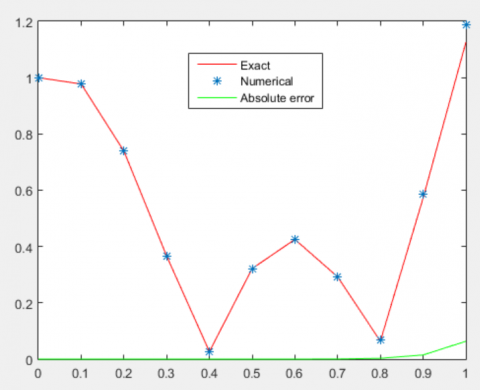
The absolute errors for mass spring system are reported in Table 3 and depicted in Figure 2.
Figure 2. Comparisons for exact, approximate and absolute errors for different mesh points for mass spring system
3.3 Elastic beam
For a beam free at both ends on an elastic foundation under the action of a distributed load w(x) the flexurat deflection y(x) is governed by the equation.
$E l y^{4}+k y=w(x)$ with the boundary conditions $y^{\prime \prime}(0)=$ $y^{\prime \prime \prime}(0)=0=y^{\prime \prime}(L)=y^{\prime \prime \prime}(L)$
In particular, let us consider the following example:
$y^{(4)}+y=e^{-x}, 0 \leq x \leq 1, y^{\prime \prime}(0)=y^{\prime \prime \prime}(0)=y^{\prime \prime}(1)$
$\quad=y^{\prime \prime \prime}(1)=0$ (20)
3.3.1 Elzaki transform
The Elzaki transform of Eq. (20), obtains:
$v^{-4} T(v)-v^{-2} y(0)-v^{-1} y^{\prime}(0)-y^{\prime \prime}(0)$$-v y^{\prime \prime \prime}(0)=E\left(e^{-x}-y\right)$$T(v)=C_{1} v^{2}+C_{2} v^{3}+v^{4} E\left(e^{-x}-y\right)$ (21)
The value of $C_{1}=y(0), C_{2}=y^{\prime}(0)$ will be determined after the series solution as in Eq. (6) is obtained.
The inverse Elzaki Transformation of Eq. (21) gives the solution as follows:
$\begin{aligned} y(x)=C_{1}+C_{2} x+E^{-1}\left[v^{4} E\left(e^{-x}-y\right)\right] \\ y(x)=e^{-x}+C_{1} &-1+\left(C_{2}+1\right) x-\frac{x^{2}}{2}+\frac{x^{3}}{3 !} \\ &-E^{-1}\left[v^{4} E(y)\right] \end{aligned}$ (22)
By MADM and Taylor’s series approximation, Eq. (22) is decomposed as:
$y_{0}=C_{1}+C_{2} x+\frac{x^{4}}{4 !}-\frac{x^{5}}{5 !}+\frac{x^{6}}{6 !}-\frac{x^{7}}{7 !}+\frac{x^{8}}{8 !}-\frac{x^{9}}{9 !}+\frac{x^{10}}{10 !}$$+O(11)$
The recurrence relation is given by:
$y_{n+1}=-E^{-1}\left[v^{4} E\left(y_{n}\right)\right]$ for $n \geq 0$
For $n=0, y_{1}=-E^{-1}\left[v^{4} E\left(y_{0}\right)\right]$
$=-E^{-1}\left(v^{4} E\left(C_{1}+C_{2} x+\frac{x^{4}}{4 !}-\frac{x^{5}}{5 !}+\frac{x^{6}}{6 !}-\frac{x^{7}}{7 !}+\frac{x^{8}}{8 !}-\frac{x^{9}}{9 !}\right.\right.$$\left.\left.+\frac{x^{10}}{10 !}\right)\right)$
$=-E^{-1}\left(v^{4}\left(C_{1} v^{2}+C_{2} v^{3}+v^{6}-v^{7}+v^{8}-v^{9}+v^{10}\right.\right.$$\left.\left.-v^{11}+v^{12}\right)\right)$$=-\left(C_{1} \frac{x^{4}}{4 !}+C_{2} \frac{x^{5}}{5 !}+\frac{x^{8}}{8 !}-\frac{x^{9}}{9 !}+\frac{x^{10}}{10 !}-\frac{x^{11}}{11 !}+\frac{x^{12}}{12 !}-\frac{x^{13}}{13 !}\right.$$\left.+\frac{x^{14}}{14 !}\right)$
For $n=1, y_{2}=C_{1} \frac{x^{8}}{8 !}+C_{2} \frac{x^{9}}{9 !}+\frac{x^{12}}{12 !}-\frac{x^{13}}{13 !}+\frac{x^{14}}{14 !}$
For $n=2, y_{3}=-C_{1} \frac{x^{12}}{12 !}-C_{2} \frac{x^{13}}{13 !}$
Substitution of the values of these components in Eq. (11), the approximate solution is:
$y(x)=C_{1}+C_{2} x+\left(1-C_{1}\right) \frac{x^{4}}{4 !}-\left(1+C_{2}\right) \frac{x^{5}}{5 !}+\frac{x^{6}}{6 !}$$-\frac{x^{7}}{7 !}$$+C_{1} \frac{x^{8}}{8 !}+C_{2} \frac{x^{9}}{9 !}+\left(1-C_{1}\right) \frac{x^{12}}{12 !}+C_{2} \frac{x^{13}}{13 !}+\cdots$ (23)
The boundary condition in Eq. (20) are substituted in Eq. (23), provides:
$\mathrm{C}_{1}=0.943127854229432$
$\mathrm{C}_{2}=-0.622264767724301$
Hence,
$y=\frac{8494940505740811}{9007199254740992}-\frac{1401215688024475}{2251799813685248} x$$+\frac{512258748000181}{216172782113783808} x^{4}$
$-\frac{850584125660773}{270215977642229760} x^{5}+\frac{1}{720} x^{6}$$-\frac{1}{5040} x^{7}$$+\frac{2831646835246937}{121056757983718932480} x^{8}$
$-\frac{280243137604895}{163426623278020558848} x^{9}$$+\frac{512258749000181}{4314462854539742753587200} x^{12}$$-\frac{56048627520979}{560880171090166557966336} x^{13}$$+\cdots$
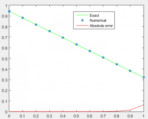
Figure 3. Comparisons of exact, approximate and absolute errors for different mesh points for elastic beam modelling
Table 3. Absolute errors for mass spring system at different mesh points
|
x |
Exact value |
Approximate value |
Absolute error |
|
0 |
1.000000000000000 |
1.000000000000000 |
0.000000000 |
|
0.1 |
0.977415978537201 |
0.977415978557043 |
1.984201691840326e-11 |
|
0.2 |
0.738971636663201 |
0.738971639214306 |
2.551104993919751e-09 |
|
0.3 |
0.366257408329042 |
0.366257455039382 |
4.671033998482344e-08 |
|
0.4 |
0.026728494238492 |
0.026727984314194 |
5.099242979984819e-07 |
|
0.5 |
0.321718076942731 |
0.321712362702702 |
5.714240029042195e-06 |
|
0.6 |
0.425350023205410 |
0.425291603001488 |
5.842020392199387e-05 |
|
0.7 |
0.292239000053105 |
0.291771119899731 |
4.678801533740118e-04 |
|
0.8 |
0.063712470035911 |
0.066638254725620 |
2.925784689709 e-03 |
|
0.9 |
0.572531110196704 |
0.587375957831336 |
1.4844847634632 e-02 |
|
1 |
1.125133170271123 |
1.188609209077959 |
6.3476038806836 e-02 |
Table 4. Absolute errors for elastic beam problem at different grid points
|
x |
Exact value |
Approximate value |
Absolute error |
|
0 |
0.943200000000000 |
0.943124474808975 |
7.552519102504984e-05 |
|
.1 |
0.880967246664593 |
0.880899363884991 |
6.788277960201317e-05 |
|
.2 |
0.818736870650345 |
0.818676710002571 |
6.016064777392138e-05 |
|
.3 |
0.756513311064063 |
0.756461038146504 |
5.227291755904862e-05 |
|
.4 |
0.694301142844698 |
0.694257015147056 |
4.412769764206015e-05 |
|
.5 |
0.632067866921078 |
0.632103494794425 |
3.562787334698836e-05 |
|
.6 |
0.569921209167234 |
0.569894537246701 |
2.667192053296130e-05 |
|
.7 |
0.507752671841497 |
0.507735517094754 |
1.715474674301998e-05 |
|
.8 |
0.445594249046082 |
0.445587280495720 |
6.968550362029813e-06 |
|
.9 |
0.383441272930632 |
0.383445269271236 |
3.996340603995563e-06 |
|
1.0 |
0.321289523969921 |
0.321305374716945 |
1.585074702398215e-05 |
All the numerical computations are carried on using Matlab and the comparison with the exact solution is reported in the Table 4 and also shown in Figure 3.
3.3.2 Mohand transforms
Taking the Mohand transform of Eq. (20).
$v^{4} R(v)-v^{5} y(0)-v^{4} y^{\prime}(0)-v^{3} y^{\prime \prime}(0)-v^{2} y^{\prime \prime \prime}(0)$$=M\left(e^{-x}-y\right)$
$v^{4} R(v)=C_{1} v^{5}+C_{2} v^{4}+M\left(e^{-x}\right)-M(y)$
$R(v)=C_{1} v+C_{2}+\frac{1}{v^{4}} M\left(e^{-x}\right)-\frac{1}{v^{4}} M(y)$
Taking the inverse Mohand transform and Taylor’s series expansion for exponential function.
$y(x)=C_{1}+C_{2} x+\frac{x^{4}}{4 !}-\frac{x^{5}}{5 !}+\frac{x^{6}}{6 !}-\frac{x^{7}}{7 !}+\frac{x^{8}}{8 !}-\frac{x^{9}}{9 !}+\frac{x^{10}}{10 !}$$-E^{-1}\left[v^{4} E(y)\right]$
By decomposition method:
$y_{0}=C_{1}+C_{2} x+\frac{x^{4}}{4 !}-\frac{x^{5}}{5 !}+\frac{x^{6}}{6 !}-\frac{x^{7}}{7 !}+\frac{x^{8}}{8 !}-\frac{x^{9}}{9 !}+\frac{x^{10}}{10 !}$
and, the recurrence relation $y_{n+1}=-M^{-1}\left[\frac{1}{v^{4}} M\left(y_{n}\right)\right], n \geq 0$ is obtained.
As earlier the components of Eq. (11) are calculated which agrees with the values calculated for Elzaki transformation. Therefore the solution derived by Mohand transformation is also same.
3.3.3 Aboodh transform
The Aboodh transform of Eq. (20), yields:
$v^{4} K(v)-v^{2} y(0)-v y^{\prime}(0)-y^{\prime \prime}(0)-\frac{1}{v} y^{\prime \prime \prime}(0)$$=A\left(e^{-x}-y\right)$
$v^{4} K(v)=C_{1} v^{2}+C_{2} v+A\left(e^{-x}\right)-A(y)$
$K(v)=C_{1} \frac{1}{v^{2}}+C_{2} \frac{1}{v^{3}}+\frac{1}{v^{4}}\left(\sum_{r=0}^{\infty}(-1)^{r} v^{r+2}\right)-\frac{1}{v^{4}} A(y)$
The inverse Aboodh transform of the above equation:
$\begin{aligned} y(x)=C_{1}+C_{2} x &+\frac{x^{4}}{4 !}-\frac{x^{5}}{5 !}+\frac{x^{6}}{6 !}-\frac{x^{7}}{7 !}+\frac{x^{8}}{8 !}-\frac{x^{9}}{9 !}+\frac{x^{10}}{10 !} \\-A^{-1}\left[\frac{1}{v^{4}} A(y)\right] \end{aligned}$
The repetition of the steps in former transforms evaluate the components of the infinite series of the Eq. (6) which are exactly equal to the ones derived by Elzaki and Mohand transform and so also the final solution.
The basic objective of this work is to implement the given transformations to linear non homogeneous differential equations in modeling occur in engineering, applied sciences and other physical phenomena The applicability and efficiency of the proposed scheme is executed by three test problems though three transformations numerically as well as graphically. The absolute error is merged with the abscissa except with some fluctuations at 0.9 and 1 as shown in Figure 2 and Figure 3 for mass spring system and elastic beam problems respectively. The present scheme can also be implemented to different branches of applied sciences for constructive modeling in the field of ordinary differential equation (ODEs) as well as partial deferential equations (PDE) in Mathematical Sciences. The proposed scheme with numerical quadrature can be implemented for electromagnetic field problems in Electronics engineering and Fracture mechanics in Civil and mechanical engineering.
[1] Zhang, J. (2007). A Sumudu based algorithm for solving differential equations. Computer Science journal of Moldova, 15(3): 303-313.
[2] Tarig, E. (2011). The new integral transform “Elzaki Transform”. Global Journal of Pure and Applied Mathematics, 7(1): 57 64.
[3] Elzaki, T.M., Elzaki, S.M. (2011). On the connections between Laplace and Elzaki transforms. Advances in Theoretical and Applied Mathematics, 6(1): 1-11.
[4] Aboodh, K.S. (2013). The new integral transform “Aboodh Transform”. Global Journal of Pure and Applied Mathematics, 9(1): 35-43.
[5] Alshikh, A.A., Abdelrahim Mahgoub, M.M. (2016). A comparative study between Laplace and two new Integral Elzaki Transform and Aboodh transform. Pure and Applied Mathematics, 5(5): 145 150. https://doi.org/10.11648/j.pamj.20160505.11
[6] Kashuri, A., Fundo, A. (2013). A new Integral transform. Advances in Theoretical and Applied Mathematics, 8(1): 303-313.
[7] Agarwal, S., Gupta, A.R. (2019). Dualities between Mohand transform and some useful integral transforms. IJRTE, 8(3): 843 847. https://doi.org/10.35940/ijrte.C4031.098319
[8] Khandelwal, R., Choudhury, P., Khandelwal, Y. (2018). Solution of fractional order differential equation by Kamal transform. International Journal of Statistics and Applied Mathematics, 3(2): 279-284.
[9] Adomian, G. (1991). A review of the decomposition method and some recent results for nonlinear problems. Computers and Mathematics with Applications, 21(5): 101-127. https://doi.org/10.1016/0898-1221(91)90220-X
[10] Jena, S.R., Dash, P. (2015). An efficient quadrature rule for approximate solution of non linear integral equation of Hammerstein type. International Journal of Applied Engineering Research,10(3): 5831-5840.
[11] Mohanty, M, Jena, S.R. (2018). Differential Transformation Method for approximate solution of ordinary differential equation. Advances in Modeling and Analysis-B, 61(3): 135-138. https://doi.org/10.18280/ama_b.610305
[12] Radid, A., Rhofir, K. (2019). Partitioning differential transformation for solving integro-differential equations problem and application to electrical circuits. Mathematical Modelling of Engineering Problems, 6(2): 235-240. https://doi.org/10.18280/mmep.060211
[13] Abdelrahim Mahgoub, M.M., Alshikh, A.A. (2017). Application of the differential transform method for the nonlinear differential equations. American Journal of Applied Mathematics, 5(1): 14-18. https://doi.org/10.11648/j.ajam.20170501.12
[14] Gebremedhin, G.S., Jena, S.R. (2019). Approximate solution of ordinary differential equation via hybrid block approach. International journal of Emerging Technology, 10(4): 201-211, 482.
[15] Jena, S.R., Mohanty, M. (2019). Numerical treatment of ODE (Fifth order). International Journal of Emerging Technology, 10(4): 191-196.
[16] Jena, S.R., Mohanty, M., Mishra, S.K. (2018). Ninth step block method for numerical solution of a fourth order ordinary differential equation. Advances in Modelling and Analysis A, 55(2): 47-56. https://doi.org/10.18280/ama_a.550202
[17] Jena, S.R., Gebremedhin, G.S. (2020), Approximate solution of a fifth order ordinary differential equation with block method. International Journal of Computing Science and Mathematics, 12(4): 413 426. https://doi.org/10.1504/IJCSM.2020.112652
[18] Mohanty, M., Jena, S.R., Mishra, S.K. (2021) Approximate solution of fourth order differential equation. Advances in Mathematics: Scientific Journal, 10(1): 621-628. https://doi.org/10.37418/amsj.10.1.62
[19] Benkharroubi, H., Mimouni, A., Bendaoud, A. (2020). Mathematical modelling of electric field generated by vertical grounding electrode in horizontally stratified soil using the FDTD method. Mathematical Modelling of Engineering Problems, 7(2): 251-257. https://doi.org/10.18280/mmep.070211
[20] Saadeh, R., Qazza, A., Burqan, A. (2020). A new integral transform: ARA transform and its properties and applications. Symmetry, 12(6): 925. https://doi.org/10.3390/sym12060925
[21] Alderremy, A.A., Elzaki, T.M., Chamekh, M. (2018). New transform iterative method for solving some Klein-Gordon equations. Results in Physics, 10: 655-659. https://doi.org/10.1016/j.rinp.2018.07.004
[22] Kamal, A., Sedeeg, H. (2016). A coupling Elzaki transform and Homotopy perturbation method for solving nonlinear fractional heat-like equations. American Journal of Mathematical and Computer Modelling, 1(1): 15-20. https://doi.org/10.11648/j.ajmcm.20160101.12
[23] Barnes, B. (2016). Polynomial integral transform for solving differential equations. European Journal of Pure and Applied Mathematics, 9(2): 140-151.
[24] Hasan, Y.Q., Zhu, L.M. (2008). Modified Adomian Decomposition method for singular initial value problems in second order differential equations. Surveys in Mathematics and its Applications, 3: 183-193.
[25] Gebremedhin, G.S., Jena, S.R. (2020). Approximate solution of a fourth order ordinary differential
equation via tenth step block method. Int. J. Computing Science and Mathematics, 11(3): 253-262. https://doi.org/10.1504/IJCSM.2020.106695
[26] Jena, S.R., Nayak, D., Acharya, M.M. (2017). Application of mixed quadrature rule on electromagnetic field problems. Computational Mathematics and Modeling, 28(2): 267-277. https://doi.org/10.1007/s10598-017-9363-4
[27] Jena, S.R., Nayak, D. (2020). Approximate instantaneous current in RLC circuit. Bulletin of Electrical Engineering and Informatics, 9(2): 803 809.
[28] Dash, P., Jena, S.R. (2015). Mixed quadrature over sphere. Global Journal of Pure and Applied Mathematics, 11(1): 415-425.
[29] Jena, S.R., Singh, A. (2015). A reliable treatment of analytic functions. International Journal of Applied Engineering Research, 10(5): 11691-11695.
[30] Jena, S.R., Mishra, S.C. (2015). Mixed quadrature for analytic functions. Global Journal of Pure and Applied Mathematics, 11(1): 281-285.
[31] Jena, S.R., Dash, P. (2015). Numerical treatment of analytic functions via mixed quadrature rule, Research Journal of Applied Sciences, Engineering and Technology, 10(4): 391-392. https://doi.org/10.19026/rjaset.10.2503
[32] Jena, S.R., Meher, K., Paul, A. (2016). Approximation of analytic functions in adaptive environment. Beni-Suef University Journal of Basic and Applied Sciences, 5(4): 306 309. https://doi.org/10.1016/j.bjbas.2016.10.001
[33] Jena, S.R., Nayak, D., Paul, A.K., Mishra, S.C. (2020). Mixed anti-Newtonian-Gaussian rule for real definite integrals. Advances in Mathematics: Scientific Journal, 9(11): 1081-1090. https://doi.org/10.37418/amsj.9.11.115
[34] Jena, S.R., Nayak, D. (2015). Hybrid quadrature for numerical treatment of nonlinear Fredholm integral equation with separable kernel. Int. J. Appl. Math. and Stat., 53(4): 83-89.
[35] Jena, S.R., Nayak, D. (2019). A comparative study of numerical integration based on mixed quadrature rule and Haar wavelets. Bull, Pure Appl. Sci. Sect. E Math. Stat., 38(2): 532-539. https://doi.org/10.5958/23203226.2019.00054.7
[36] Jena, S.R., Singh, A. (2019). A Mathematical Model for Approximate Solution of Line Integral. Journal of Computer and Mathematical Sciences, 10(5): 1163-1172.
[37] Meher, K., Jena, S.R., Paul, A.K. (2017). Approximate Solution of real definite integrals in adaptive routine. Indian Journal of Science and Technology, 10(5): 1-4. https://doi.org/10.17485/ijst/2017/v10i5/93871
[38] Jena, S.R., Dash, P. (2014). Approximation of Real definite integral via hybrid quadrature domain. International Journal of Science Engineering Technology and Research, 3(12): 3188 3191.
[39] Singh, A., Jena, S.R., Mishra, B.B. (2017). Mixed quadrature rule for double integrals. International Journal of Pure and Applied Mathematics, 117(1): 1-9. https://doi.org/10.12732/ijpam. v117i1.1
[40] Jena, S.R., Singh, A. (2018). Approximation of real definite integration. International Journal of Advanced Research in Engineering and Technology, 9(4): 197-207.
[41] Dash, R.B., Jena, S.R. (2009). Multidimensional integral of several real variables. Bulletin of Pure and Applied Sciences, 28: 147-154.
[42] Dash, R.B., Jena, S.R. (2008). A mixed quadrature of modified Birkhoff Young using Richardson extrapolation and Gauss Legendre 4 point transformed rule. International Journal of Applied Mathematics and Application, 2: 111-117.
[43] Jena, S.R., Dash, R.B. (2009). Mixed quadrature of real definite integrals over triangles. Pacific-Asian Journal of Mathematics, 3(1-2): 119-124.
[44] Mishra, S.C., Jena, S.R. (2018). Approximate evaluation of analytic functions through extrapolation. International Journal of Pure and Applied Mathematics, 118(3): 791-800. https://doi.org/10.12732/ijpam.v118i3.24
[45] Mohanty, P.K., Hota, M.K., Jena, S.R. (2014). A comparative study of mixed quadrature rule with the compound quadrature rules. American International Journal of Reaserch in Science, Technology, Engineering Mathematics, 7(1): 45-52.
[46] Nayak, D., Jena, S.R., Acharya, M.M. (2017). Approximate solution of muntz system. Global Journal of Pure and Applied Mathematics, 13(7): 3013-3020.
[47] Erwin Kreyszig 8th edition, John Wiley and Sons. Inc., 1988.
[48] Jena, S.R., Senapati, A., Gebremedhin, G.S. (2020). Numerical study of solitions in BFRK scheme. International Journal of Mechanics and Control, 21(2): 163-175.
[49] Jena, S.R., Senapati, A., Gebremedhin, G.S. (2020). Approximate solution of MRLW equation in B-spline environment. Mathematical Sciences, 14(3): 345-357. https://doi.org/10.1007/s40096-020-00345-6
[50] Jena, S.R., Gebremedhin, G.S. (2021). Decatic B-spline collocation scheme for approximate solution of Burgers’ equation. Numerical Methods for Partial Differental Equations. https://doi.org/10.1002/num.22747
[51] Jena, S.R., Gebremedhin, G.S. (2021). Computational technique for heat and advection–diffusion equations. Soft Computing. https://doi.org/10.1007/s00500-021-05859-2