Omar Lakdar![]() | Louay Elsoufi
| Louay Elsoufi![]() | Marwan Alkheir
| Marwan Alkheir![]() | Hassan Assoum*
| Hassan Assoum*![]() | Kamel Abed-Meraim
| Kamel Abed-Meraim![]() | Anas Sakout
| Anas Sakout![]()
© 2025 The authors. This article is published by IIETA and is licensed under the CC BY 4.0 license (http://creativecommons.org/licenses/by/4.0/).
OPEN ACCESS
Modeling and analyzing the complex flow behavior of impinging jets is essential for many engineering applications, especially due to their highly nonlinear and unsteady nature. Traditional modeling approaches often face difficulties in accurately capturing the evolving features of such flows. In this study, a data-driven framework is developed to extract and analyze hidden structures from experimental data of a rectangular air jet impinging on a flat surface at a Reynolds number of 6700. The dataset consists of time-resolved velocity fields obtained using Time-Resolved Particle Image Velocimetry (TR-PIV). A convolutional autoencoder (AE) architecture is employed to compress the high-dimensional flow field into a latent space of 256 variables. This latent representation captures the essential dynamic features of the jet while enabling accurate reconstruction of the original velocity fields. Temporal analysis of the latent variables reveals structured patterns associated with coherent flow dynamics. Furthermore, spectral analysis of selected latent components highlights dominant frequency peaks consistent with vortex shedding in the impingement region. These results demonstrate the capability of convolutional autoencoders to uncover physically meaningful patterns in complex fluid flows and offer a promising tool for data-driven flow analysis.
impinging jet, convolutional neural networks, autoencoders, PIV measurements, vortex shedding
Many studies have been conducted to explore the complex physics of impinging jet flow and to analyze the influence of various flow parameters. For instance, Assoum et al. [1] provided detailed investigations into the fundamental characteristics governing impinging jet behavior [2]. Further analyses of the flow field associated with jet impingement on flat surfaces have been reported by previous study, among others, who focused on the interaction between the jet and the impingement surface and its effect on flow structures and turbulence [3].
More recently, a notable feedback mechanism controlling high-speed subsonic impinging jets at the nozzle exit has been identified and studied extensively [4, 5]. These investigations have provided important insights into the dynamic coupling between the jet exit conditions and the impingement region, which significantly affects the flow stability and noise generation [6, 7].
Impinging jets find widespread utility in many industrial and engineering applications due to their superior convective heat and mass transfer capabilities. Common areas of application include cooling of gas turbine blades, electronic component thermal management, drying in paper and textile industries, and aerodynamic flow control. The ability of impinging jets to provide localized high heat transfer rates makes them indispensable in processes demanding efficient thermal regulation and surface treatment [8, 9].
Traditionally, such flow phenomena have been studied using computational fluid dynamics (CFD) methods, including Reynolds-Averaged Navier-Stokes (RANS), Large Eddy Simulation (LES), and Direct Numerical Simulation (DNS). While DNS can offer highly accurate results, its computational demands make it impractical for many real-world problems, especially at high Reynolds numbers. LES provides a middle ground but still requires considerable resources for capturing near-wall turbulence and transient dynamics. RANS remains the most computationally efficient option but is often inadequate for resolving unsteady, nonlinear features common in impinging jet flows. In contrast, deep learning offers a data-driven, model-free alternative capable of reconstructing complex flow fields directly from experimental data, significantly reducing computation time once trained. This makes DL particularly attractive for high-dimensional, time-resolved flow problems like jet impingement.
In recent years, deep learning has emerged as a powerful tool for modeling and analyzing complex physical systems, particularly those involving multiscale and nonlinear dynamics. Architectures such as convolutional neural networks (CNNs) and long short-term memory (LSTM) networks have demonstrated significant capabilities in capturing spatial and temporal correlations, making them especially valuable in fluid mechanics research. DL has found increasing application in areas like turbulence modeling, flow dynamics prediction, and the reconstruction of flow fields from sparse or noisy data.
One of the most impactful developments has been the use of DL for enhancing experimental fluid measurements, such as particle image velocimetry (PIV). Super-resolution techniques based on CNNs and generative adversarial networks (GANs) have been successfully applied to recover high-resolution velocity fields from low-resolution inputs, significantly improving the quality of reconstructed data [10]. These methods are particularly useful in scenarios where direct access to high-fidelity measurements is limited or infeasible. Additionally, autoencoder-based networks have shown strong potential in estimating flow fields with missing regions, offering a non-intrusive and efficient alternative to traditional model-based approaches.
Despite these advancements, challenges remain regarding the interpretability and generalizability of deep neural networks, especially in data-limited environments. Current efforts aim to develop hybrid methods that integrate physical constraints with data-driven learning to improve reliability and transparency in DL-based fluid flow models [11, 12].
In this study, a neural network based on the autoencoder architecture was applied to extract essential flow structures and enable efficient reconstruction of the velocity field associated with jet dynamics. The influence of latent space dimensionality on reconstruction fidelity was systematically examined [13]. Furthermore, to gain insight into the dynamic behavior of the flow, the frequency content of the transverse velocity was analyzed at a representative location characterized by the presence of coherent vortex structures.
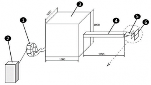
The experimental setup is designed to investigate subsonic impinging jet flows and associated control strategies as shown in Figure 1. Air is supplied by an external compressor regulated by a Siemens MICROMASTER 420 frequency inverter, allowing adjustment of the jet exit velocity up to 33 m/s (Mach ≈ 0.1). The airflow passes through a 1 m³ settling chamber equipped with grids and honeycomb structures to reduce turbulence and align the flow. It then enters a 1250 mm long rectangular duct (190 mm × 90 mm) that leads to a fourth-order polynomial nozzle with an exit height of 10 mm and width of 190 mm, yielding an aspect ratio of 19.
The jet impacts an aluminum plate (250 mm × 250 mm, 4 mm thick) with a central slit matching the nozzle dimensions. In a circular jet configuration, the nozzle-to-plate distance is set to L/D = 2.08, where D = 7.8 mm represents the jet exit diameter. The Reynolds number, based on D and the jet exit velocity, is Re = 6700. In the slit jet case, the impact distance L is adjustable via a precision linear stage (ISEL MS 200 HT2 Direkt) with 0.01 mm accuracy, and is controlled using Galaad software. The dimensionless impact distance L/H is varied during the experiments.
For flow control, a 4 mm diameter rod is introduced between the jet and the plate. The rod is scanned through 1085 spatial positions in the X-Y plane using two automated linear stages controlled by a LabVIEW program. At each position, acoustic measurements are performed with a 15 kHz sampling rate over 3 seconds, following a stabilization period to reduce mechanical noise. Each full scan, corresponding to one Reynolds number, is followed by automatic adjustment of the air velocity for the next configuration.
Velocity field measurements are conducted using Particle Image Velocimetry (PIV). The flow is seeded with olive oil droplets generated by a LaVision Laskin Nozzle aerosol generator. The droplets, with diameters between 0.1–0.2 μm, are sufficiently small to follow the turbulent structures without affecting the flow. The PIV system captures consecutive images of the seeded flow illuminated by a laser sheet, enabling 2D velocity field reconstruction through cross-correlation. This non-intrusive technique allows analysis of the jet’s coherent structures and their role in noise generation.
Figure 1. Experimental setup: (1) Compressor, (2) variable frequency drive, (3) settling chamber, (4) duct, (5) rectangular convergent outlet, and (6) slotted plate [3]
This study relies on a deep learning-based approach to predict and reconstruct velocity fields of a circular air jet impinging on a flat surface. The methodology involves several key steps: experimental data acquisition, velocity field preprocessing, autoencoder model design and training, followed by latent space analysis and validation of the reconstructed results.
Prior to training the model, raw velocity fields are structured as spatiotemporal tensors. Each data sample consists of two channels corresponding to the horizontal and vertical velocity components, defined over a fixed spatial grid. A normalization procedure is applied to center the data and improve model convergence.
To reduce noise and enhance learning efficiency, the velocity fields are also filtered using thresholding or spatial smoothing techniques when necessary.
In this study, a convolutional neural network (CNN) based on the U-Net architecture is implemented, inspired by the works of Ribeiro et al. [14]. U-Net is an encoder–decoder architecture particularly well-suited for capturing complex spatial structures and reconstructing high-dimensional data [15].
The network consists of four encoder–decoder blocks. Each encoder block includes two convolutional layers: the first followed by a ReLU (Rectified Linear Unit) activation, and the second followed by another ReLU and a MaxPooling layer, which reduces spatial resolution while extracting hierarchical features. The first two encoder blocks employ convolutional kernels of size 5, with strided convolutions in the first layer to downsample the input. The last two blocks use smaller kernels (size 3) to retain more spatial detail while continuing the compression process.
In Figure 2, the decoding phase mirrors the encoding process, applying upsampling operations followed by convolutional layers to progressively restore the original resolution. Skip connections are used to concatenate feature maps between corresponding encoder and decoder blocks, helping preserve spatial information and improve reconstruction accuracy.
At the bottleneck of the network, a 256-dimensional latent representation encodes the essential spatiotemporal structures of the velocity field. The model was implemented in Python using the Deep Learning Toolbox [16]. Training was conducted over 100 epochs with a batch size of 16, minimizing the mean squared error (MSE) loss using the Adam optimizer.
Figure 2. U-Net architecture
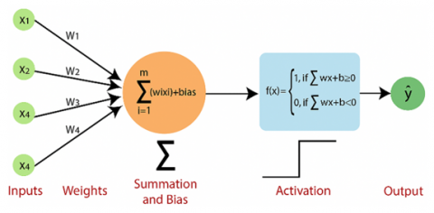
In this study, the weights and biases of the convolutional neural network are the key learnable parameters optimized during training (Figure 3). They play a crucial role in the network’s ability to capture complex nonlinear relationships embedded in the measured velocity fields.
Each convolutional filter is associated with a set of weights that define how local features of the input—such as gradients or flow structures—are detected and propagated through the layers. Bias terms are added to the outputs of convolution operations to shift activation thresholds independently of the input, providing the network with greater flexibility to model subtle variations.
These parameters are initialized randomly and iteratively updated during training by minimizing the mean squared error (MSE) loss function using the Adam optimization algorithm. The update process is governed by the backpropagation algorithm, which computes the gradient of the loss with respect to each parameter and adjusts them in the opposite direction of the gradient.
This optimization cycle is repeated over multiple epochs—100 in our case—until the model converges and achieves optimal performance on the velocity field reconstruction task.
While this study adopts a U-Net-based convolutional autoencoder due to its strong performance in image-to-image regression tasks, alternative deep learning architectures have shown promise in fluid dynamics applications.
For instance, a Transformer trained with self-supervised learning has been shown to reconstruct and predict complex flow fields using sparse labeled data [17]. Another study proposed an Energy Transformer specifically to reconstruct full velocity fields from highly incomplete measurements—up to 90% missing data—with impressive accuracy [18]. Hybrid models like CFD former, combining Vision Transformers with U-Nets, have also outperformed traditional architectures in fluid flow approximations. Moreover, the recently introduced Fluid Former architecture melds continuous convolution with Transformer-style attention, achieving strong stability in complex fluid simulations [19]. However, these models typically require larger datasets and higher computational resources. In our case, U-Net provided a good balance between complexity, spatial resolution, and training stability, making it suitable for reconstructing PIV-based velocity fields. Future work may explore hybrid sindy, PINS or Transformer-based models to assess their potential benefits in terms of reconstruction accuracy and interpretability [20].
Figure 3. Weights-biases configuration
6.1 Velocity field prediction
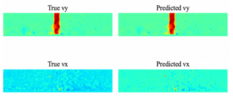
Figure 4 presents a qualitative comparison between the true velocity components and those reconstructed by the convolutional neural network (CNN) model, trained to predict the horizontal (vx) and vertical (vy) components of the flow field in a jet impingement configuration.
Figure 4. Visualization of the actual and CNN-reconstructed velocity components of the flow field
The top row of the figure displays both the actual and predicted distributions of the vertical and horizontal velocity components. The CNN demonstrates a strong ability to reproduce the central features of the flow, particularly the high-velocity jet core and the surrounding regions where velocity gradually decreases. The model accurately captures the spatial structure of the flow, including fine-scale features and coherent patterns.
The bottom row illustrates the prediction of the horizontal component vx, which generally exhibits lower amplitude and more diffuse structures compared to vy. Despite these challenges, the predicted fields show a high degree of spatial correlation with the ground truth, successfully reproducing both the large-scale distribution and finer variations.
These results highlight the capability of the CNN to effectively learn the complex spatiotemporal dynamics of turbulent jet flows. The close agreement between the predicted and actual velocity fields, especially on previously unseen test data, confirms the model’s generalization capacity and its potential for data-driven flow reconstruction tasks.
6.2 Spatial prediction error analysis
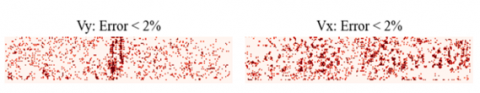
Figure 5 presents spatial maps of relative prediction error for the velocity components vx and vy at the time instant 50. The maps highlight pixels where the predicted velocities differ by less than 2% from the true values. Areas shown in red indicate regions where the convolutional neural network (CNN) achieves high prediction accuracy.
On the left, the map for the vertical velocity component (vy) reveals a broad distribution of pixels with errors below 2%. The CNN demonstrates strong performance across much of the domain, particularly near the flow boundaries and in background regions, where the vertical velocity component tends to be weaker and less complex.
On the right, the error map for the horizontal component (vx) shows a dense concentration of low-error pixels along the jet axis. This indicates that the model accurately captures the horizontal velocity behavior in the jet’s high-velocity core, a region critical for maintaining the flow’s structural integrity. The prevalence of low-error predictions in this central area underscores the robustness and reliability of the CNN model.
Overall, these spatial error analyses confirm that the CNN provides reliable predictions of both velocity components, maintaining low relative error across dynamically significant regions of the flow field.
Figure 5. Relative error map (< 2%) for the velocity components vx and vy
6.3 Temporal evolution of the latent vector
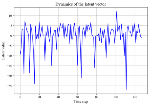
Figure 6 depicts the temporal evolution of a latent vector extracted from the autoencoder at each time step. This vector encapsulates the essential dynamics of the velocity field through a compressed representation learned during the training process.
The observed oscillations in the latent vector reflect temporal variations in the encoded flow characteristics, with distinct peaks around specific time steps (e.g., near 60 and 105). These peaks correspond to significant flow events or disturbances, likely associated with transitions in the jet structure or turbulent activity near the vortex core.
These findings indicate that the autoencoder effectively encodes critical flow dynamics, particularly in the vortex-jet interaction region. The latent space evolution captures the nonlinear behavior governed by the underlying partial differential equations of the impinging jet flow, demonstrating the model’s ability to represent unsteady flow phenomena over time.
In this system, the impinging jet and vortex dynamics introduce nonlinearities into both velocity components, especially near the centerline or obstacle. This results in strong gradients, time-dependent interactions, and occasional symmetry breaking. Such effects directly manifest as fluctuations in the latent vector, especially during periods of vortex movement or intensification.
Figure 6. Temporal evolution of a latent vector
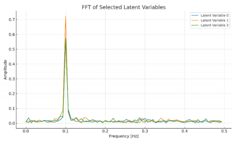
Figure 7. (FFT) temporal evolution of selected latent variables
To assess whether the latent space encodes meaningful flow dynamics, we applied a Fast Fourier Transform (FFT) to the temporal evolution of selected latent variables. The resulting power spectra exhibit distinct peaks at specific frequencies, consistent with the expected periodic behavior of vortex shedding in impinging jet flows. This indicates that the autoencoder effectively captures the temporal characteristics of the jet’s coherent structures. A representative FFT plot of three latent variables is shown in Figure 7, demonstrating their oscillatory nature and confirming the physical relevance of the encoded features.
6.4 Global latent space analysis, training convergence, and vorticity field reconstruction
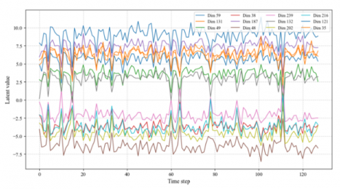
To further understand the internal representations learned by the convolutional neural network (CNN) trained to predict the velocity field, the temporal evolution of the 256-dimensional latent vector was analyzed. As depicted in Figure 8, each curve represents the trajectory of a single latent variable throughout the time sequence. Extracted from the network’s bottleneck layer, these latent variables encapsulate the essential spatiotemporal features required for accurate velocity field reconstruction.
Figure 8. Temporal evolution of a latent vector
The temporal dynamics exhibited by these latent variables are rich and varied, with several showing oscillatory or quasi-periodic patterns. This behavior indicates that the CNN effectively captures recurrent motifs in the flow evolution. Variations in amplitude across variables suggest differing sensitivities to input dynamics, with some latent variables encoding dominant flow features and others capturing subtler, localized variations. Notably, a subset of variables clusters near zero, hinting at potential redundancy or underutilization within the latent representation. This structured and dynamic latent behavior validates the choice of a 256-dimensional latent space. Complementary analyses, such as principal component analysis or clustering, could further assess redundancy and inform potential dimensionality reduction.
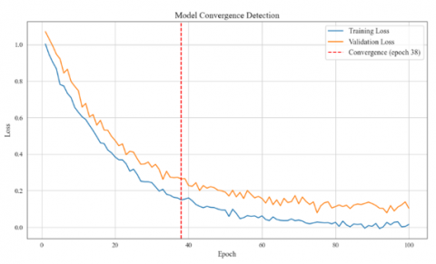
Figure 9 presents the CNN’s convergence behavior during training on approximately 1500 samples. Both training and validation losses decrease sharply in the initial phase, demonstrating rapid learning of meaningful flow patterns. Subsequently, losses stabilize near zero, indicating that the network attains a stable and precise internal representation. The close alignment of training and validation losses beyond the convergence point confirms the model’s robust generalization to unseen data.
Figure 9. CNN’s convergence behavior during training
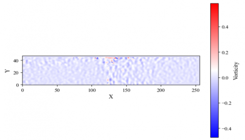
Expanding beyond velocity field reconstruction, the CNN’s capability to predict higher-order flow quantities is demonstrated in Figure 10, which displays the predicted vorticity field. This field captures the spatial distribution of rotational flow structures, with positive and negative vorticity regions highlighted. The model’s architecture enables it to discern fine turbulent details and coherent structures inherent in fluid flows, proving effective in reconstructing complex flow dynamics beyond simple velocity vectors. Accurate vorticity prediction represents a significant advancement, as it is critical for understanding shear layers, vortex interactions, and energy dissipation mechanisms in fluid systems. The success of this approach underscores both the robustness of the latent space representation and the effectiveness of the training strategy employed.
Figure 10. Predicted vorticity field
The velocity field of impinging jets was successfully predicted using a deep learning-based approach relying on convolutional autoencoders (AEs). These models were trained to learn compact latent representations of the flow and accurately reconstruct its spatiotemporal behavior. The velocity data were obtained experimentally using Particle Image Velocimetry (PIV) at a Reynolds number of Re = 6700. The results demonstrate that the flow dynamics can be effectively reproduced using a reduced number of latent variables. Moreover, the spectral analysis of these latent variables revealed dominant frequency peaks that match those found in the transverse velocity spectrum at locations where coherent vortices pass, highlighting a strong correlation between the learned features and the underlying vortex dynamics.
While the trained model shows high accuracy in reconstructing and predicting the velocity field, some limitations remain. Prediction errors were primarily observed in regions with flow separation and strong nonlinear interactions, particularly in the transverse velocity component. Nevertheless, the model showed excellent performance in periodic regions of the flow, suggesting that it successfully captures the dominant coherent structures.
Some local inaccuracies remain in highly nonlinear regions, such as separation bubbles, due to the complex and intermittent nature of turbulent structures. However, the nonlinear behavior observed in the latent space reflects these dynamics faithfully rather than indicating model failure. Future work will explore methods to improve local accuracy in these challenging zones.
Future improvements could focus on refining the model's ability to generalize in more complex flow regimes, especially near separation zones. Furthermore, the current framework can be extended to include parametric inputs such as the Reynolds number or nozzle geometry, enabling generalized flow field prediction under varying conditions. A promising direction would also be the integration of wall-based sensor data (e.g., wall shear stress) as input to predict full-field flow dynamics.
Future research will also focus on embedding interpretability into the model architecture, through feature attribution, latent space analysis, and physics-informed training strategies.
This could eventually contribute to predictive modeling tools for real-time flow control, heat transfer optimization, and energy efficiency applications in engineering systems.
[1] Assoum, H.H., Hassan, M.E., Abed-Meraïm, K., Martinuzzi, R., Sakout, A. (2013). Experimental analysis of the aero-acoustic coupling in a plane impinging jet on a slotted plate. Fluid Dynamics Research, 45(4): 045503. https://doi.org/10.1088/0169-5983/45/4/045503
[2] Zang, Y., Street, R.L., Koseff, J.R. (1993). A dynamic mixed subgrid-scale model and its application to turbulent recirculating flows. Physics of Fluids A: Fluid Dynamics, 5(12): 3186–3196. https://doi.org/10.1063/1.858675
[3] Assoum, H.H., Hamdi, J., Alkheir, M., Meraim, K.A., Sakout, A., Obeid, B., El Hassan, M. (2021). Tomographic particle image velocimetry and dynamic mode decomposition (DMD) in a rectangular impinging jet: Vortex dynamics and acoustic generation. Fluids, 6(12): 429. https://doi.org/10.3390/fluids6120429
[4] Assoum, H.H., Hamdi, J., Abed-Meraïm, K., El Hassan, M., Ali, M., Sakout, A. (2017). Correlation between the acoustic field and the transverse velocity in a plane impinging jet in the presence of self-sustaining tones. Energy Procedia, 139: 391–397. https://doi.org/10.1016/j.egypro.2017.11.227
[5] El Hassan, M., Assoum, H.H., Sobolik, V., Vétel, J., Abed-Meraim, K., Garon, A., Sakout, A. (2012). Experimental investigation of the wall shear stress and the vortex dynamics in a circular impinging jet. Experiments in Fluids, 52(6): 1475–1489. https://doi.org/10.1007/s00348-012-1269-5
[6] Hamdi, J., Assoum, H., Abed-Meraïm, K., Sakout, A. (2018). Volume reconstruction of an impinging jet obtained from stereoscopic-PIV data using POD. European Journal of Mechanics - B/Fluids, 67: 433–445. https://doi.org/10.1016/j.euromechflu.2017.09.001
[7] Assoum, H.H., Hamdi, J., Abed-Meraïm, K., Al Kheir, M., Mrach, T., El Soufi, L., Sakout, A. (2019). Spatio-temporal changes in the turbulent kinetic energy of a rectangular jet impinging on a slotted plate analyzed with high speed 3D tomographic-particle image velocimetry. International Journal of Heat and Technology, 37(4): 1071-1079. https://doi.org/10.18280/ijht.370416
[8] Alotaibi, H.M., El Hassan, M., Assoum, H.H., Meraim, K.A., Sakout, A. (2020). A review paper on heat transfer and flow dynamics in subsonic circular jets impinging on rotating disk. Energy Reports, 6: 834-842. https://doi.org/10.1016/j.egyr.2020.11.124
[9] El Hassan, M., Nobes, D.S. (2022). Experimental investigation of the vortex dynamics in circular jet impinging on rotating disk. Fluids, 7(7): 223. https://doi.org/10.3390/fluids7070223
[10] Deng, Z., He, C., Liu, Y., Kim, K.C. (2019). Super-resolution reconstruction of turbulent velocity fields using a generative adversarial network-based artificial intelligence framework. Physics of Fluids, 31(12): 125111. https://doi.org/10.1063/1.5127031
[11] Vinuesa, R., Brunton, S.L. (2022). Enhancing computational fluid dynamics with machine learning. Nature Computational Science, 2(6): 358-366. https://doi.org/10.1038/s43588-022-00264-7
[12] Nathan Kutz, J. (2017). Deep learning in fluid dynamics. Journal of Fluid Mechanics, 814: 1-4. https://doi.org/10.1017/jfm.2016.803
[13] Duraisamy, K., Iaccarino, G., Xiao, H. (2019). Turbulence modeling in the age of data. Annual Review of Fluid Mechanics, 51(1): 357-377. https://doi.org/10.1146/annurev-fluid-010518-040547
[14] Ribeiro, M.D., Rehman, A., Ahmed, S., Dengel, A. (2021). DeepCFD: Efficient steady-state laminar flow approximation with deep convolutional neural networks. arXiv: arXiv:2004.08826. https://doi.org/10.48550/arXiv.2004.08826
[15] Thuerey, N., Weißenow, K., Prantl, L., Hu, X. (2020). Deep learning methods for Reynolds-averaged Navier–stokes simulations of airfoil flows. AIAA Journal, 58(1): 25-36. https://doi.org/10.2514/1.J058291
[16] Oliphant, T.E. (2007). Python for scientific computing. Computing in Science & Engineering, 9(3): 10-20. https://doi.org/10.1109/MCSE.2007.58
[17] Zhang, Q., Krotov, D., Karniadakis, G.E. (2025). Operator learning for reconstructing flow fields from sparse measurements: an energy transformer approach. arXiv:2501.08339. https://doi.org/10.48550/ARXIV.2501.08339
[18] Kang, H., Kim, Y., Le, T.T.H., Choi, C., Hong, Y., Hong, S., Chin, S.W., Kim, H. (2023). A new fluid flow approximation method using a vision transformer and a U-shaped convolutional neural network. AIP Advances, 13(2): 025233. https://doi.org/10.1063/5.0138515
[19] Wang, N.Y., Chen, Y., Zheng, S. (2025). FluidFormer: Transformer with continuous convolution for particle-based fluid simulation. arXiv:2508.01537. https://doi.org/10.48550/ARXIV.2508.01537
[20] Raissi, M., Perdikaris, P., Karniadakis, G.E. (2019). Physics-informed neural networks: A deep learning framework for solving forward and inverse problems involving nonlinear partial differential equations. Journal of Computational Physics, 378: 686-707. https://doi.org/10.1016/j.jcp.2018.10.045