Mariela J. Quispe![]() | Noemi Callirgos | Segundo Sánchez
| Noemi Callirgos | Segundo Sánchez![]() | Henry Sandoval | David Coronel-Bustamante
| Henry Sandoval | David Coronel-Bustamante![]() | Luis Perez-Delgado
| Luis Perez-Delgado![]() | Yashira Oliva
| Yashira Oliva![]() | Victor H. Taboada-Mitma
| Victor H. Taboada-Mitma![]() | Juancarlos Cruz-Luis
| Juancarlos Cruz-Luis![]() | Alejandro Seminario-Cunya
| Alejandro Seminario-Cunya![]() | Annick E. Huaccha-Castillo
| Annick E. Huaccha-Castillo![]() | Nilton Atalaya-Marin
| Nilton Atalaya-Marin![]() | Darwin Gomez-Fernandez
| Darwin Gomez-Fernandez![]() | Franklin H. Fernandez-Zarate*
| Franklin H. Fernandez-Zarate*![]()
© 2025 The authors. This article is published by IIETA and is licensed under the CC BY 4.0 license (http://creativecommons.org/licenses/by/4.0/).
OPEN ACCESS
The Shumba watershed, located in the province of Jaén, played an essential role in the ecological balance and water supply of the region. The objective of this study was to analyze changes in land cover and land use between 1998 and 2024, using spectral indices of vegetation, soil, and water derived from Landsat 5 and 8 images. The processing was performed in Google Earth Engine and ArcGIS 10.5, applying the Random Forest algorithm for supervised classification. The results indicate an increase of 2708.11 ha in the category “Mosaic of crops, pastures and natural spaces” and 122.50 ha in “Continuous urban fabric”. In contrast, reductions were recorded in “Shrub/herbaceous vegetation” (-1867.32 ha), “High dense forest” (-462.86 ha), “Transient crops” (-446.25 ha), and “Bare land” (-54.17 ha). Validation of the classification yielded an overall accuracy of 0.90 and a Kappa coefficient of 0.88, which supports the reliability of the results. These changes show significant transformations in the landscape, providing key information for territorial planning and the implementation of environmental conservation policies.
remote sensing, Google Earth Engine (GEE), Landsat, LULC
As globalization, climate change, consumption, and population growth exert greater pressure on finite land resources, it is essential to understand and monitor the drivers of these changes, as well as the ecological implications, from local to global scales [1]. The expansion of agriculture plays an important role in the transformation of the landscape, causing significant challenges for the conservation of different ecosystems around the world. Statements indicate that the agricultural area could increase by 14% between 2010 and 2030; this would generate greater pressure on forested areas and/or shrub vegetation [2, 3].
Land cover and land use (LULC) changes are generated by biological, physical and social interactions; endogenous and exogenous factors; technological advances; economic and population growth, following a stochastic behavior [4-6]. These changes turn out to be negative, mainly for the existing biodiversity and functioning of ecosystems. Furthermore, erosion processes and loss of soil fertility, decrease in water quality, and loss of habitats are enhanced; consequently, it ends up affecting the provision of environmental goods and services [6-8].
Watersheds are important natural hydrological units that allow the storage and transport of water resources and nutrients throughout their area, while supporting different ecological communities [9, 10]. Changes in the volume and rate of runoff resulting from variations in land use and land cover can erode the soil and thereby increase the amount of sediment transported, generating flooding problems in the lower areas of the watershed [11]. In that sense, the ecosystem function of flood control and water purification is affected; therefore, to ensure the proper functioning of these ecosystems, it is necessary that resource management and conservation include analysis of land cover and land use changes in watersheds [12].
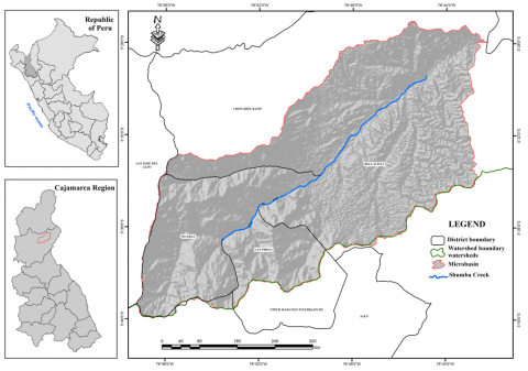
The Shumba watershed, with an area of 34204.39 ha, plays a strategic role in providing key ecosystem services for the districts of Jaen, San Jose del Alto, Huabal, Las Pirias, and Bellavista. This watershed is integrated into the hydrographic system of the Chinchipe River, which contributes significantly to the flow of the Marañon River, a major tributary of the Amazon Basin. From a hydrological perspective, the Shumba watershed supplies water to more than 40000 inhabitants [13] and irrigates nearly 1500 ha of agricultural land (Junta de Usuarios del Sector Hidraulico Menor Jaén – San Ignacio), making it an essential source for human consumption, family agriculture, and productive activities in the area. In addition, its surface flows have been identified as contributing to the stability of the Marañón water regime, especially during the dry season, acting as a natural regulator in the face of climate variability [14].
This basin harbors remnants of tropical montane forest and areas of highly diverse herbaceous vegetation, which provide critical habitats for different species. Several investigations on biodiversity in montane ecosystems indicate that the altitudinal gradients present in the Shumba basin promote high ecological heterogeneity, favoring critical biological corridors for migratory birds and local fauna [15]. In addition, recent studies show that inter-Andean watersheds with remnant forest cover, such as Shumba, play a relevant role in carbon sequestration, erosion mitigation, and provision of clean water [16, 17]. These functions are key to addressing the cumulative impacts of climate change, agricultural expansion, and urban sprawl [18, 19]. Given its ecological, functional, and hydrological relevance, the Shumba watershed represents a priority unit for scientific research, natural resource conservation, and sustainable territorial planning in the context of the tropical Andes.
Large-scale and long-term monitoring methodologies are closely linked to the dynamic analysis of LULC transformations through time and space [20]. Land use and land cover mapping information is a primary source of information that serves for different research related to the earth system, including studies of biodiversity, climate change, public health, carbon cycle [21, 22], and also provides important information for planning urban expansion and natural resource management [23].
Remote sensing represents an essential technology for the analysis of land cover changes at the regional, continental or global level [24]. Landsat 5 (1998) and Landsat 8 (2024) satellite images offer consistent historical coverage, adequate spatial resolution (30 m) for regional studies, and are freely available through the Google Earth Engine (GEE) platform. Although sensors such as Sentinel-2 present higher spatial resolution, their limited coverage since 2015 restricts their usefulness for extensive multitemporal analyses.
Previous studies have validated the use of the Landsat series for land use monitoring and long-term change detection [25, 26], especially in tropical regions with complex cloud conditions. Also, the implementation of GEE-based tools allows for efficient management of large volumes of data, facilitating reproducible and regional-scale analyses [20, 27].
In this context, this research aims to i) analyze the spatial and temporal changes in land cover and land use in the Shumba watershed between 1998 and 2024, using satellite imagery and supervised classification techniques, ii) evaluate the accuracy of the supervised classification using the Random Forest algorithm, and iii) identify the main conversion and persistence processes between LULC classes using transition matrices.
2.1 Location of the study area
The Shumba watershed has an area of 34204.39 ha, covering part of the districts of San Jose del Alto, Jaen, Huabal, Las Pirias, and Bellavista, province of Jaen, Cajamarca region. Hydrographically, Shumba is part of the Chinchipe Basin and the Upper Marañon III Interbasin (Figure 1). It is located at parallels 5° 40' 0'' and 5° 28' 0'' south latitude and meridians 78° 56' 0'' and 78° 44' 0'' west longitude, with an altitudinal gradient that ranges between 372 and 2464 m.a.s.l.
Figure 1. Location of the Shumba watershed
2.2 Methodological design
Figure 2 shows the methodological flowchart to determine land cover and land use changes in the study area, using remote sensing techniques and geographic information systems (GIS).
Figure 2. Methodological flowchart to determine the land cover and land use in the Shumba watershed in the district and province of Jaen-Cajamarca
2.3 Spatial information
The study area was delimited using a vector file (shapefile) of Shumba Creek and a digital elevation model (DEM) from the Shuttle Radar Topography Mission (SRTM) with a spatial resolution of 30 meters, available on the Google Earth Engine platform [28]. This information was processed in the ArcGIS 10.5 software.
The temporal analysis covered the years 1998 and 2024. Landsat 5 and Landsat 8 satellite images (level 2, collection 2) were used, with a spatial resolution of 30 m and a maximum cloud cover of 30%. The images were obtained from the United States Geological Survey (USGS) (Table 1) repository and processed using the Google Earth Engine platform [27].
Table 1. Description of Landsat 5 and Landsat 8 data acquired
|
Name |
Name |
Scale |
Wavelength (μm) |
Description |
|
Landsat 5 |
SR_B1 |
2.75e- 05 |
0.45- 0.52 |
Band 1 surface reflectance (blue) |
|
SR_B2 |
2.75e-05 |
0.52-0.60 |
Band 2 surface reflectance (green) |
|
|
SR_B3 |
2.75e-05 |
0.63-0.69 |
Band 3 surface reflectance (red) |
|
|
SR_B4 |
2.75e-05 |
0.77-0.90 |
Band 4 surface reflectance (near infrared) |
|
|
SR_B5 |
2.75e-05 |
1.55-1.75 |
Band 5 surface reflectance (shortwave infrared 1) |
|
|
SR_B7 |
2.75e-05 |
2.08-2.35 |
Band 7 surface reflectance (shortwave infrared 2) |
|
|
Landsat 8 |
SR_B1 |
2.75e- 05 |
0.435-0.451 |
Band 1 surface reflectance (ultra-blue, coastal aerosol) |
|
SR_B2 |
2.75e-05 |
0.452-0.512 |
Band 2 surface reflectance (blue) |
|
|
SR_B3 |
2.75e-05 |
0.533-0.590 |
Band 3 surface reflectance (green) |
|
|
SR_B4 |
2.75e-05 |
0.636-0.673 |
Band 4 surface reflectance (red) |
|
|
SR_B5 |
2.75e-05 |
0.851-0.879 |
Band 5 surface reflectance (near infrared) |
|
|
SR_B6 |
2.75e-05 |
1.566-1.651 |
Band 6 surface reflectance (shortwave infrared 1) |
|
|
SR_B7 |
2.75e-05 |
2.107-2.294 |
Band 7 surface reflectance (shortwave infrared 2) |
2.4 Obtaining LULC maps
For supervised classification, the Random Forest algorithm [29] was applied, which constructs multiple decision trees to generate a final class by majority voting. Hundred trees were set up (ntree=100) and √m (where m is the number of predictor variables) was used as the mtry value, following the recommendations for multispectral analysis [30].
To ensure a statistically robust representation, homogeneous and well-defined training areas were identified and selected to prominently represent the spectral and spatial characteristics of each land use and land cover class. The selection process was carried out using simplified random sampling, which allowed us to adequately capture the internal variability of each class and maximize the representativeness of the samples in the classifier training. In total, 18 training areas were used, with a cumulative surface of 477 pixels, covering all the defined thematic classes. For validation, 18 independent areas, equivalent to 44% of the total number of training pixels, with an area of 369 pixels, were used. This proportion guarantees an objective and statistically consistent evaluation of the performance of the supervised classification model [31], which was followed for all classes except the airport class, where it was performed manually.
LULC classes were defined according to the Corine Land Cover methodology adapted for Peru, and include: continuous urban fabric (Tuc), airports (Ae), transient crops (Ct), crop mosaic, pasture and natural spaces (Mcpen), tall dense forest (Bda), shrub/herbaceous vegetation (Var/Her) and bare land (Td) (Table 2) [32].
Table 2. Land cover and land use were identified in the Shumba watershed
|
LEVEL I |
LEVEL II |
LEVEL III |
CODE |
|
1. Artificialized areas |
1.1 Urbanized areas |
1.1.1 Continuous urban fabric |
|
|
1.2 Industrial areas and infrastructure |
1.2.4 Airports |
||
|
2. Agricultural areas |
2.1 Transient crops |
--- |
|
|
2.4 Heterogeneous agricultural areas |
2.4.3 Mosaic of crops, pastures, and natural spaces |
||
|
3. Forests and mostly natural areas |
3.1 Forests |
3.1.3 High dense forest |
|
|
3.3 Areas with herbaceous and/or shrub vegetation |
3.3.4 Shrub / herbaceous vegetation |
||
|
3.4 Areas without or with little vegetation |
3.4.3 Bare lands |
Source: Adapted from study [32].
2.5 Spectral indices
The following spectral indices were used: NDVI, EVI, SAVI, BSI, NDMI, and MNDWI (Table 3). The use of Enhanced Vegetation Index (EVI) was prioritized over NDVI and NDVIre due to its better performance in areas with high vegetation cover, such as the Shumba watershed. EVI minimizes the saturation effect of NDVI in dense cover and is less sensitive to atmospheric and soil interference [33]. The NDVIre index was not considered since it requires bands in the red-edge region, absent in Landsat sensors.
Table 3. Spectral indices used
|
Name |
Abbreviation |
Formula |
Source |
|
Normalized Difference Vegetation Index |
NDVI |
$\boldsymbol{N} \boldsymbol{D V I}=\frac{N I R-R E D}{N I R+R E D}$ |
[34] |
|
Improved Vegetation Index |
EVI |
$\boldsymbol{E} \boldsymbol{V} \boldsymbol{I}=C \times\left[\frac{(N I R-R E D)}{(N I R+C 1 × R E D-C 2 × B L U E+L)}\right]$ |
[35] |
|
Soil Adjusted Vegetation Index |
SAVI |
$\boldsymbol{S A V I}=\left[\frac{(N I R-R E D)}{(N I R+R E D+L)}\right] × (1+L)$ |
[36] |
|
Bare Soil Index |
BSI |
$\boldsymbol{B} \boldsymbol{S I}=\frac{[(R E D+S W I R)-(N I R+B L U E)]}{[(R E D+S W I R)+(N I R+B L U E)]}$ |
[37] |
|
Modified Normalized Difference Water Index |
MNDWI |
$M N D W I=\frac{(G R E E N-S W I R 1)}{(G R E E N+S W I R 1)}$ |
[38] |
|
Normalized Difference Moisture Index |
NDMI |
$\boldsymbol{N D M I}=\frac{(N I R-S W I R 1)}{(N I R+S W I R 1)}$ |
[39] |
*where, C=2.5; C1=6; C2=7.5; L=0.5
2.6 Thematic accuracy
Classification accuracy was evaluated using confusion matrices, calculating overall accuracy, errors of commission and omission, and the Kappa index [40-42].
The Kappa index evaluates whether the classification has accurately discriminated the categories of interest, being calculated with Eq. (1) [43].
$k=\frac{m \sum_{i=1 ; n} X_{i i}-\sum_{i=1 ; n} X_{i+} X_{+i}}{m^2-\sum_{i=1 ; n} X_{i+} X_{+i}}$ (1)
where, n is the number of rows of the matrix, Xii is the number of observations in row i and column i; Xi+ and X+i are the end of row i and column i, and m is the total number of observations.
2.7 Spatial-temporal intensity of the rate of change and transition matrices
The cross-tabulation matrix was developed to determine the annual rate of change (S) using Eq. (2) applied by FAO [44] and to calculate losses or gains of land cover and land use classes.
$S=\left(\frac{S_1}{S_1}\right)^{\frac{1}{t_2-t_1}}-1$ (2)
where, S1 and S2 are the dates at t1 and t2, a negative value S is evidence of a decrease in LULC, and if it is greater than zero, it indicates an increase in LULC.
The transition matrix (Table 4) shows the land cover and land use classes distributed on the horizontal and vertical axes, corresponding to times t1 and t2, respectively. The cells located on the diagonal indicate the areas that remained unchanged between the two periods, while the other cells reflect the areas that were transformed from one class to another during the interval analyzed. In addition, the table includes a final row and column that sums the total areas of all classes recorded in t1 and t2.
Table 4. Transition matrix, rate of change (S), and rates of change for the 7-land cover and land use classes of the study area for the period 1998-2024 (area in ha and %)
|
2024 |
Total 1998 (ha) |
Rate of Change |
Loss (Li) |
Total Change (Ct) |
Net Change (Cn) |
Exchange (Int) |
|||||||
|
Tuc |
Ae |
Ct |
Mcpen |
Bda |
Var/ Her |
Td |
% |
||||||
|
Tuc |
67.08 |
38.06 |
6.18 |
6.64 |
117.96 |
2.78 |
43.13 |
190.12 |
103.85 |
86.27 |
|||
|
Ae |
|
45.01 |
4.00 |
49.01 |
0.00 |
8.16 |
16.30 |
0.02 |
16.28 |
||||
|
Ct |
109.72 |
2.38 |
4663.15 |
1304.42 |
9.78 |
6089.45 |
-0.29 |
23.42 |
39.52 |
7.33 |
32.19 |
||
|
Mcpen |
33.55 |
6927.63 |
22.10 |
39.99 |
7023.27 |
1.26 |
1.36 |
41.28 |
38.56 |
2.72 |
|||
|
Bda |
484.96 |
148.31 |
633.27 |
-4.92 |
76.58 |
80.07 |
73.09 |
6.98 |
|||||
|
Var/Her |
30.11 |
1.61 |
938.19 |
2312.61 |
16820.81 |
31.20 |
20134.53 |
-0.37 |
16.46 |
23.64 |
9.27 |
14.37 |
|
|
Td |
3.80 |
91.35 |
61.75 |
156.90 |
-1.62 |
60.64 |
86.76 |
34.53 |
52.24 |
||||
|
Total 2024 (ha) |
240.46 |
49.00 |
5643.20 |
9731.38 |
170.41 |
18267.21 |
102.73 |
34204.39 |
|||||
|
Gain (Gj) (%) |
146.98 |
8.14 |
16.09 |
39.92 |
3.49 |
7.18 |
26.12 |
||||||
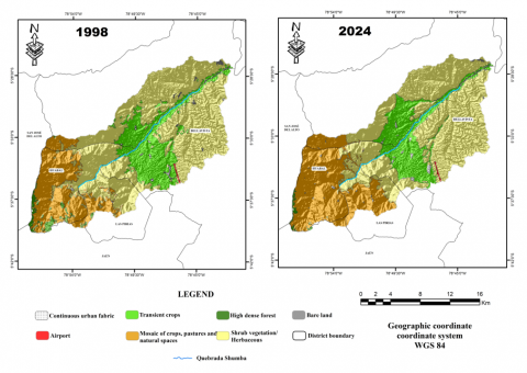
3.1 Land cover and land use maps
Figure 3 shows the land cover and land use maps for the years 1998 and 2024 in the Shumba watershed, district, and province of Jaen. Of the seven classes identified, the increase of Mosaic of pasture crops and natural spaces is observed due to land use change of continuous urban fabric, deforestation of high dense forest and herbaceous shrub vegetation; on the other hand, continuous urban fabric in its expansion took areas of transitory crops, mosaic of pasture crops and natural spaces and herbaceous shrub vegetation.
Figure 3. Map of land cover and land use in the Shumba watershed, district and province of Jaen
The coverages that decreased their area are: shrub/herbaceous vegetation as the expansion took place continuous urban fabric, airport, transitory crop, mosaic of pasture crops and natural spaces, bare land; tall dense forest was replaced by mosaic of pasture crops and natural spaces, transitory crops part of its area went to the classes of bare land, continuous urban fabric, herbaceous shrub vegetation; likewise, bare land decreased its area due to the expansion of transitory crops and shrub/Herbaceous vegetation.
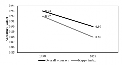
The precision values of the generated maps were obtained by elaborating the confusion matrix for both years, which allowed the comparison of the Global Accuracy and Kappa index, whose values for the year 1998 were 0.93 and 0.92, while for the year 2024 presented a Global Accuracy of 0.90 and a Kappa index of 0.88 (Figure 4).
Figure 4. Global precision values and kappa index for the Shumba watershed
3.2 Rate of change (S)
It is observed that the estimated rates for the period 1998-2024 show marked changes in land cover and land use. The positive rate of change is shown for Tuc (2.78%) and Mcpen (1.26%), which increased in extent, due to the loss of other cover classes, e.g., Ct (-0.29%) and Var/Her (-0.37%). The reduction of Bda, which presents a higher negative annual rate of change (-4.92%) due to the increase of Mcpen, followed by Td (-1.62%) due to the extension of the Ct and Var/Her boundary (Table 4).
3.3 Evaluation of land cover and land use changes
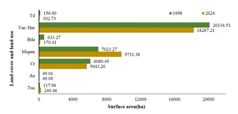
3.3.1 At the period and surface level
The spatial-temporal dynamics of land cover and land use (LULC) of the Shumba watershed in the 26-year period showed an increase of 7.92% (2708.11 ha), in mosaic crops, pastures and natural spaces, 0.36% (122.50 ha) continuous urban fabric, and, as for the classes that present loss in their area were shrub/herbaceous vegetation -5.46% (-1867.32 ha), high dense forest -1.35% (-462.86 ha), transitory crop -1.30% (-446.25 ha) and bare land -0.16% (-54.17 ha), the class that did not present variation in its area is airports (Table 5 and Figure 5).
Table 5. Land cover and land use in the Shumba watershed, 1998-2024
|
Land Cover and Land Use (LULC) |
Symbology |
1998 |
% |
2024 |
% |
1998-2024 |
% |
|
Continuous urban fabric |
117.96 |
0.34 |
240.46 |
0.70 |
122.50 |
0.36 |
|
|
Airports |
49.01 |
0.14 |
49.00 |
0.14 |
-0.01 |
0.00 |
|
|
Transient crops |
6089.45 |
17.80 |
5643.20 |
16.50 |
-446.25 |
-1.30 |
|
|
Mosaic of crops, pastures, and natural spaces |
7023.27 |
20.53 |
9731.38 |
28.45 |
2708.11 |
7.92 |
|
|
Highly dense forest |
633.27 |
1.85 |
170.41 |
0.50 |
-462.86 |
-1.35 |
|
|
Shrub/Herbaceous vegetation |
20134.53 |
58.87 |
18267.21 |
53.41 |
-1867.32 |
-5.46 |
|
|
Bare lands |
156.90 |
0.46 |
102.73 |
0.30 |
-54.17 |
-0.16 |
|
|
Total |
34204.39 |
100 |
34204.39 |
100 |
|||
Figure 5. Spatial-temporal dynamics of land cover and land use classes in the Shumba watershed, 1998-2024
3.3.2 At the level of change indices
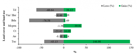
The Tuc and Mcpen classes had the greatest change in area in the Shumba watershed (net change) of 103.85% and 38.56% (Table 4), with area gains of 146.98% and 39.92%, respectively (Figure 6). Likewise, the classes Bda, Td, Var/Her, Ct, Ae, presented net changes of 73.09%, 34.53%, 9.27%, 7.33%, 0.02% (Table 4) over the 26-year period, with losses ranging from -76.58%, -60.64%, -16.46%, -23.42%, and -8.16%, respectively (Figure 6).
Figure 6. Gains and losses of land cover and land use classes in the Shumba watershed, 1998-2024
3.3.3 At the level of transitions by classes
Through the analysis of the transition matrices, it is observed that the Var/Her transformation was generated by the expansion of Tuc (30.11 ha), Ae (1.61 ha), Ct (938.19 ha), Mcpen (2312.61 ha) and Td (31.20 ha); Bda was towards a process of expansion of the Mcpen mosaic border (484.96 ha), on the other hand, Ct were transformed to Td (9.78 ha), Tuc (109.72 ha), Ae (2.38 ha), Var/Her (1304.42 ha); finally, Td changed to Ct (3.8 ha) and Var/Her (91.35 ha) (Table 4).
The results of the Global Accuracy and Kappa index showed acceptable accuracy values (Kappa index between 0.88 and 0.92 and Global Accuracy between 0.90 and 0.93), for the case of the global accuracy of the maps exceeded 80% (indicated as minimum threshold for a reliable land cover and land use classification [45-47], similar results were observed in the Kappa statistic which showed strong correlation between the classified map and the actual values on the ground, accurately reflecting the land cover and land use in the Shumba watershed [48], in general, it can be stated that through the methodology used it is possible to generate cartographic information with spatial and temporal coherence [41, 46, 49, 50], however, the maps generated are often subject to errors of commission and omission [51]; for this study, errors of commission were minimized through the use of NDVI which allows analyzing changes generated in vegetation cover [51-53], while omission errors are related to the spatial resolution, which can underestimate or overestimate other land uses [51], therefore, it was chosen to use Landsat 5 and Landsat 8 satellite images, with a spatial resolution of 30 m and maximum cloudiness of 30%.
The results of the study show that Mcpen and Var/Her are the coverages with the greatest distribution in the Quebrada Shumba watershed for the two years of study (1998-2024). A clear dynamic is shown in the surface changes of these two coverages. For the case of Var/Her, the loss was 1867.32 ha for the period of analysis, being the reflection of the 2708.11 ha increase of Mcpen [6, 54].
In the case of Tuc and Mcpen, these are the two coverages that increased in area by 2024 with respect to the area reported in 1998. Tuc increased by 122.5 ha, while Mcpen increased by 2708.11 ha, while Bda decreased by 462.86 ha, and Var/Her decreased by 1867.32 ha. These results are in agreement with those reported in different research studies which indicate that the advance of the agricultural and livestock frontier, replacing forests with crops and/or pastures, and urban expansion tend to decimate wooded and/or shrub areas, decreasing the areas for natural regeneration, as can be seen in the results of the present research, in which an increase in Tuc was observed (+122.50 ha / +0.36%) which is a clear indicator of the urbanization process within the watershed associated mainly with population growth [41, 49].
Spatial analysis showed a positive correlation between urban growth and population increase in districts such as Jaén, where a 35% increase was recorded between 1993 and 2017 according to [13]. The expansion of the continuous urban fabric (Tuc) was greater in the vicinity of main access roads, reflecting the concentrated urbanization pattern. Furthermore, correlation analysis between LULC change and distance to urban centers and rivers suggests that socioeconomic factors and geographic accessibility are key drivers of change [5, 55]. Finally, the area in Ct (-446.25 ha / -1.30%) and Td (-54.17 ha / -0.16%) decreased; the former could be associated with land use change towards perennial crops, soil degradation, which generates the abandonment of these lands, effects of climate change; while the latter could suggest that some degraded soils have recovered or reforested and/or are colonized by natural vegetation or crops.
The results obtained in the Shumba basin reflect a regional pattern of transformation of the Andean landscape, associated with agricultural expansion, deforestation, and unplanned urbanization. Studies such as those of findings in study [41] in livestock micro-watersheds in Amazonas and study [50] in the La Leche river basin show similar conversion patterns. Likewise, research in high Andean watersheds in Ecuador and Bolivia has reported accelerated loss of forest cover due to agricultural advancement and population pressure [16, 18].
These dynamics respond to socioeconomic factors, such as the demand for productive land, disjointed agricultural policies and internal migratory processes, leading to a constant expansion of the areas, which could lead to loss of biodiversity, erosion, change of microclimates and contamination of soil and water resources, affecting people's livelihoods [49], this highlights the need for integrated regional territorial management strategies. The factors that influence LULC changes have varied over time. Initially, these processes were mainly determined by natural conditions, such as slope, altitude, soil type, and proximity to water sources. However, nowadays, human influence has become more relevant, highlighting aspects such as economic development, public policies, and technological advances [55, 56].
The use of remote sensing has been key to monitor changes in land cover and land use, providing a clear picture of the current state of the study area [46, 57], however, in recent years new technologies have emerged that have significantly expanded analysis capabilities, such as Google Earth Engine (GEE), radar imagery, and Remotely Piloted Aircraft Systems (RPAS) [41], which can incorporate hyperspectral cameras and machine learning algorithms for more accurate and detailed assessment.
The delimitation of an agroecological “red line” is proposed in areas where more than 30% of the agricultural mosaic has been replaced by urban areas or degraded lands. This line should be used to establish buffer strips with incentives for agroforestry practices and ecological restoration, especially in the middle parts of the watershed. In addition, it is recommended that compensation mechanisms for ecosystem services be implemented for producers who conserve remnants of native vegetation, as a strategy for sustainable territorial governance [58].
An important limitation of the present study is the use of single-phase images (one season per year), which prevents us from fully capturing the seasonal variability of dynamic land covers such as transient crops or herbaceous vegetation. It is recommended that future research integrate multi-temporal series in different climatic seasons (dry and wet), with sensors such as Sentinel-2, which allow higher temporal frequency and spectral resolution useful to distinguish phenological variations [59, 60].
The multitemporal analysis of land cover and land use in the Shumba watershed between 1998 and 2024 showed significant transformations, dominated by the increase in the mosaic of crops, pastures, and natural spaces (+2708.11 ha) and the expansion of the continuous urban fabric (+122.50 ha). These changes occurred at the expense of shrub/herbaceous vegetation, tall dense forest, and transient crops, indicating a trend towards the loss of natural ecosystems and increasing anthropic pressure on the territory's resources. The supervised classification using Random Forest showed high levels of precision (0.90-0.93), validating the reliability of the maps generated. As an action measure, it is recommended to implement an active restoration strategy of at least 500 ha of high-density forest in areas of high loss, prioritizing areas with medium slopes and high ecological fragility. It is also proposed to establish an “agroecological red line” to protect at least 1,500 ha of agricultural mosaics with potential for urban conversion, applying compensation mechanisms for ecosystem services and land use regulation. The results of this study not only constitute a robust technical basis for territorial planning in the Shumba basin, but also a strategic input for designing policies for the conservation, restoration, and sustainable use of Andean ecosystems in the face of the challenges of global change.
The authors thank the Instituto Nacional de Innovacion Agraria (INIA) through the Investment Project with CUI N° 2472675 entitled: Improvement of Research Services and Transfer of Agricultural Technology at the Baños del Inca Agricultural Experimental Station, Baños del Inca, located in the district of Baños del Inca, province of Cajamarca, department of Cajamarca.
[1] Lambin, E.F., Geist, H.J. (2008). Land-Use and land-Cover Change: Local Processes and Global Impacts. Springer Science & Business Media.
[2] Glinskis, E.A., Gutiérrez-Vélez, V.H. (2019). Quantifying and understanding land cover changes by large and small oil palm expansion regimes in the Peruvian Amazon. Land Use Policy, 80: 95-106. https://doi.org/10.1016/j.landusepol.2018.09.032
[3] Schneider, U.A., Havlík, P., Schmid, E., Valin, H., et al. (2011). Impacts of population growth, economic development, and technical change on global food production and consumption. Agricultural Systems, 104(2): 204-215. https://doi.org/10.1016/j.agsy.2010.11.003
[4] Chu, H.J., Lin, Y.P., Huang, C.W., Hsu, C.Y., Chen, H.Y. (2010). Modelling the hydrologic effects of dynamic land-use change using a distributed hydrologic model and a spatial land-use allocation model. Hydrological Processes, 24(18): 2538-2554. https://doi.org/10.1002/hyp.7667
[5] Lambin, E.F., Geist, H.J., Lepers, E. (2003). Dynamics of land-use and land-cover change in tropical regions. Annual Review of Environment and Resources, 28: 205-241. https://doi.org/10.1146/annurev.energy.28.050302.105459
[6] Nené-Preciado, A.J., González Sansón, G., Mendoza Cantú, M.E., de Asís Silva Bátiz, F. (2017). Cambio de cobertura y uso de suelo en cuencas tropicales costeras del Pacífico central Mexicano. Investigaciones Geográficas, 94. https://doi.org/10.14350/rig.56770
[7] Freeman, M.C., Pringle, C.M., Jackson, C.R. (2007). Hydrologic connectivity and the contribution of stream headwaters to ecological integrity at regional scales. JAWRA Journal of the American Water Resources Association, 43(1): 5-14. https://doi.org/10.1111/j.1752-1688.2007.00002.x
[8] Peña-Cortés, F., Escalona-Ulloa, M., Pincheira-Ulbrich, J., Rebolledo, G. (2011). Land use change in the geosystem coastal basin of the Boroa river (Chile) between 1994 and 2004. Revista de la Facultad de Ciencias Agrarias. Universidad Nacional de Cuyo, 43(2).
[9] Amindin, A., Siamian, N., Kariminejad, N., Clague, J.J., Pourghasemi, H.R. (2024). An integrated GEE and machine learning framework for detecting ecological stability under land use/land cover changes. Global Ecology and Conservation, 53: e03010. https://doi.org/10.1016/j.gecco.2024.e03010
[10] Lane, C.R., Creed, I.F., Golden, H.E., Leibowitz, S.G., et al. (2023). Vulnerable waters are essential to watershed resilience. Ecosystems, 26: 1-28. https://doi.org/10.1007/s10021-021-00737-2
[11] Issaka, S., Ashraf, M.A. (2017). Impact of soil erosion and degradation on water quality: A review. Geology, Ecology, and Landscapes, 1(1): 1-11. https://doi.org/10.1080/24749508.2017.1301053
[12] Desta, H., Fetene, A. (2020). Land-use and land-cover change in Lake Ziway watershed of the Ethiopian Central Rift Valley Region and its environmental impacts. Land Use Policy, 96: 104682. https://doi.org/10.1016/j.landusepol.2020.104682
[13] INEI. (2017). Perú: Perfil Sociodemográfico. Informe Nacional. Censos Nacionales 2017: XII de Población, VII de Vivienda y III de Comunidades Indígenas. https://www.inei.gob.pe/biblioteca-virtual/publicaciones-digitales/, accessed 2-6-2025.
[14] Whitley, R., Taylor, D., Macinnis-Ng, C., Zeppel, M., Yunusa, I., O’Grady, A., Froend, R., Medlyn, B., Eamus, D. (2013). Developing an empirical model of canopy water flux describing the common response of transpiration to solar radiation and VPD across five contrasting woodlands and forests. Hydrological Processes, 27(8): 1133-1146. https://doi.org/10.1002/hyp.9280
[15] McMichael, C.H., Bush, M.B., Silman, M.R., Piperno, D.R., Raczka, M., Lobato, L.C., Zimmerman, M., Hagen, S., Palace, M. (2013). Historical fire and bamboo dynamics in western Amazonia. Journal of Biogeography, 40(2): 299-309. https://doi.org/10.1111/jbi.12002
[16] Buytaert, W., Célleri, R., De Bièvre, B., Cisneros, F., Wyseure, G., Deckers, J., Hofstede, R. (2006). Human impact on the hydrology of the Andean páramos. Earth-Science Reviews, 79(1): 53-72. https://doi.org/10.1016/j.earscirev.2006.06.002
[17] Drobyshev, I., Ryzhkova, N., Niklasson, M., Zhukov, A., Mullonen, I., Pinto, G., Kryshen’, A. (2022). Marginal imprint of human land use upon fire history in a mire-dominated boreal landscape of the Veps Highland, North-West Russia. Forest Ecology and Management, 507: 120007. https://doi.org/10.1016/j.foreco.2022.120007
[18] Zimmerer, K.S. (2010). Biological diversity in agriculture and global change. Annual Review of Environment and Resources, 35: 137-166. https://doi.org/10.1146/annurev-environ-040309-113840
[19] McDonnell, J.J., McGuire, K., Aggarwal, P., Beven, K.J., et al. (2010). How old is streamwater? Open questions in catchment transit time conceptualization, modelling and analysis. Hydrological Processes, 24(12): 1745-1754. https://doi.org/10.1002/hyp.7796
[20] Chen, C., Yang, X., Jiang, S., Liu, Z. (2023). Mapping and spatiotemporal dynamics of land-use and land-cover change based on the Google Earth Engine cloud platform from Landsat imagery: A case study of Zhoushan Island, China. Heliyon, 9(9): e19654. https://doi.org/10.1016/j.heliyon.2023.e19654
[21] Luo, M., Hu, G., Chen, G., Liu, X., Hou, H., Li, X. (2022). 1 km land use/land cover change of China under comprehensive socioeconomic and climate scenarios for 2020–2100. Scientific Data, 9: 110. https://doi.org/10.1038/s41597-022-01204-w
[22] Zafar, Z., Zubair, M., Zha, Y., Fahd, S., Ahmad Nadeem, A. (2024). Performance assessment of machine learning algorithms for mapping of land use/land cover using remote sensing data. The Egyptian Journal of Remote Sensing and Space Sciences, 27(2): 216-226. https://doi.org/10.1016/j.ejrs.2024.03.003
[23] Ammann, L., Bosem-Baillod, A., Eckerter, P.W., Entling, M.H., Albrecht, M., Herzog, F. (2022). Comparing floral resource maps and land cover maps to predict predators and aphid suppression on field bean. Landscape Ecology, 37(2): 431-441. https://doi.org/10.1007/s10980-021-01361-0
[24] Wang, C., Yang, Q., Zhang, C., Li, X., Chen, J., Zhang, X., Chen, J., Liu, K. (2022). Rice-fish-duck system regulation of soil phosphorus fraction conversion and availability through organic carbon and phosphatase activity. Frontiers in Environmental Science, 10. https://doi.org/10.3389/fenvs.2022.979234
[25] Wulder, M.A., Masek, J.G., Cohen, W.B., Loveland, T.R., Woodcock, C.E. (2012). Opening the archive: How free data has enabled the science and monitoring promise of Landsat. Remote Sensing of Environment, 122: 2-10. https://doi.org/10.1016/j.rse.2012.01.010
[26] Roy, D.P., Wulder, M.A., Loveland, T.R., Woodcock, C.E., et al. (2014). Landsat-8: Science and product vision for terrestrial global change research. Remote Sensing of Environment, 145: 154-172. https://doi.org/10.1016/j.rse.2014.02.001
[27] Gorelick, N., Hancher, M., Dixon, M., Ilyushchenko, S., Thau, D., Moore, R. (2017). Google earth engine: Planetary-scale geospatial analysis for everyone. Remote Sensing of Environment, 202: 18-27. https://doi.org/10.1016/j.rse.2017.06.031
[28] Farr, T.G., Rosen, P.A., Caro, E., Crippen, R., et al. (2007). The shuttle radar topography mission. Reviews of Geophysics, 45(2). https://doi.org/10.1029/2005RG000183
[29] Breiman, L. (2001). Random forests. Machine Learning, 45: 5-32. https://doi.org/10.1023/A:1010933404324
[30] Belgiu, M., Drăguţ, L. (2016). Random forest in remote sensing: A review of applications and future directions. ISPRS Journal of Photogrammetry and Remote Sensing, 114: 24-31. https://doi.org/10.1016/j.isprsjprs.2016.01.011
[31] Foody, G.M. (2002). Status of land cover classification accuracy assessment. Remote Sensing of Environment, 80(1): 185-201. https://doi.org/10.1016/S0034-4257(01)00295-4
[32] MINAM. (2014). Análisis de las Dinámicas de Cambio de Cobertura de la Tierra en la Comunidad Andina. https://www.gob.pe/institucion/minam/informes-publicaciones/2714-analisis-de-las-dinamicas-de-cambio-de-cobertura-de-la-tierra-en-la-comunidad-andina.
[33] Huete, A., Didan, K., Miura, T., Rodriguez, E.P., Gao, X., Ferreira, L.G. (2002). Overview of the radiometric and biophysical performance of the MODIS vegetation indices. Remote Sensing of Environment, 83(1): 195-213. https://doi.org/10.1016/S0034-4257(02)00096-2
[34] Rouse Jr, J.W., Haas, R.H., Schell, J.A., Deering, D.W. (1973). Monitoring the vernal advancement and retrogradation (green wave effect) of natural vegetation (No. NASA-CR-132982).
[35] Gao, X., Huete, A.R., Didan, K. (2003). Multisensor comparisons and validation of MODIS vegetation indices at the semiarid Jornada experimental range. IEEE Transactions on Geoscience and Remote Sensing, 41(10): 2368-2381. https://doi.org/10.1109/TGRS.2003.813840
[36] Huete, A.R. (1988). A soil-adjusted vegetation index (SAVI). Remote Sensing of Environment, 25(3): 295-309. https://doi.org/10.1016/0034-4257(88)90106-X
[37] Rikimaru, A., Sarathi, P., Miyatake, S. (2002). Tropical forest cover density mapping. Tropical Ecology, 43(1): 39-47.
[38] McFeeters, S.K. (1996). The use of the Normalized Difference Water Index (NDWI) in the delineation of open water features. International Journal of Remote Sensing, 17(7): 1425-1432. https://doi.org/10.1080/01431169608948714
[39] Wilson, E.H., Sader, S.A. (2002). Detection of forest harvest type using multiple dates of Landsat TM imagery. Remote Sensing of Environment, 80(3): 385-396. https://doi.org/10.1016/S0034-4257(01)00318-2
[40] Chuvieco, E. (2020). Fundamentals of Satellite Remote Sensing (3rd Edition.). CRC Press. https://doi.org/10.1201/9780429506482
[41] Marin, N.A., Barboza, E., López, R.S., Vásquez, H.V., et al. (2022). Spatiotemporal dynamics of grasslands using landsat data in livestock micro-watersheds in Amazonas (NW Peru). Land, 11(5): 674. https://doi.org/10.3390/land11050674
[42] Padilla, M., Stehman, S.V., Chuvieco, E. (2014). Validation of the 2008 MODIS-MCD45 global burned area product using stratified random sampling. Remote Sensing of Environment, 144: 187-196. https://doi.org/10.1016/j.rse.2014.01.008
[43] Pontius Jr, R.G., Shusas, E., McEachern, M. (2004). Detecting important categorical land changes while accounting for persistence. Agriculture, Ecosystems & Environment, 101(2): 251-268. https://doi.org/10.1016/j.agee.2003.09.008
[44] FAO. (1996). Evaluaciones de recursos forestales mundiales: Evaluación de los recursos forestales 1990. https://www.fao.org/forest-resources-assessment/past-assessments/fra-1990/es/.
[45] Deribew, K.T., Dalacho, D.W. (2019). Land use and forest cover dynamics in the North-eastern Addis Ababa, central highlands of Ethiopia. Environmental Systems Research, 8: 8. https://doi.org/10.1186/s40068-019-0137-1
[46] Mulatu, K., Hundera, K., Senbeta, F. (2024). Analysis of land use/ land cover changes and landscape fragmentation in the Baro-Akobo Basin, Southwestern Ethiopia. Heliyon, 10(7): e28378. https://doi.org/10.1016/j.heliyon.2024.e28378
[47] Thomlinson, J.R., Bolstad, P.V., Cohen, W.B. (1999). Coordinating methodologies for scaling landcover classifications from site-specific to global: steps toward validating global map products. Remote Sensing of Environment, 70(1): 16-28. https://doi.org/10.1016/S0034-4257(99)00055-3
[48] Lillesand, T., Kiefer, R.W., Chipman, J. (2015). Remote Sensing and Image Interpretation. John Wiley & Sons.
[49] Do, A.N.T., Tran, H.D., Ashley, M., Nguyen, A.T. (2022). Monitoring landscape fragmentation and aboveground biomass estimation in Can Gio Mangrove Biosphere Reserve over the past 20 years. Ecological Informatics, 70: 101743. https://doi.org/10.1016/j.ecoinf.2022.101743
[50] Vera, E., Cruz, C., Barboza, E., Salazar, W., Canta, J., Salazar, E., Vásquez, H.V., Arbizu, C.I. (2024). Change of vegetation cover and land use of the Pómac forest historical sanctuary in northern Peru. International Journal of Environmental Science and Technology, 21(14): 8919-8930. https://doi.org/10.1007/s13762-024-05597-6
[51] Parente, L., Ferreira, L. (2018). Assessing the spatial and occupation dynamics of the brazilian pasturelands based on the automated classification of MODIS images from 2000 to 2016. Remote Sensing, 10(4): 606. https://doi.org/10.3390/rs10040606
[52] Anand, A., Pandey, P.C., Petropoulos, G.P., Pavlides, A., et al. (2020). Use of hyperion for mangrove forest carbon stock assessment in bhitarkanika forest reserve: A contribution towards blue carbon initiative. Remote Sensing, 12(4): 597. https://doi.org/10.3390/rs12040597
[53] Gitelson, A.A. (2004). Wide dynamic range vegetation index for remote quantification of biophysical characteristics of vegetation. Journal of Plant Physiology, 161(2): 165-173. https://doi.org/10.1078/0176-1617-01176
[54] Mas Caussel, J.F., Osorio, L.P., Guerra, F., Maass, M. (2015). Análisis y modelación de los procesos de deforestación: Un caso de estudio en la cuenca del río Coyuquilla, Guerrero, México. Investigaciones Geográficas, 88. https://doi.org/10.14350/rig.43853
[55] Chávez, A.B., Broadbent, E.N., Almeyda Zambrano, A.M. (2014). Smallholder policy adoption and land cover change in the southeastern Peruvian Amazon: A twenty-year perspective. Applied Geography, 53: 223-233. https://doi.org/10.1016/j.apgeog.2014.06.017
[56] Schweizer, P.E., Matlack, G.R. (2014). Factors driving land use change and forest distribution on the coastal plain of Mississippi, USA. Landscape and Urban Planning, 121: 55-64. https://doi.org/10.1016/j.landurbplan.2013.09.003
[57] Ali, I., Cawkwell, F., Dwyer, E., Barrett, B., Green, S. (2016). Satellite remote sensing of grasslands: from observation to management. Journal of Plant Ecology, 9(6): 649-671. https://doi.org/10.1093/jpe/rtw005
[58] Pagiola, S., Arcenas, A., Platais, G. (2005). Can payments for environmental services help reduce poverty? An exploration of the issues and the evidence to date from Latin America. World Development, 33(2): 237-253. https://doi.org/10.1016/j.worlddev.2004.07.011
[59] Zhu, Z., Woodcock, C.E., Olofsson, P. (2012). Continuous monitoring of forest disturbance using all available landsat imagery. Remote Sensing of Environment, 122: 75-91. https://doi.org/10.1016/j.rse.2011.10.030
[60] Li, F., Song, G., Zhu, L., Zhou, Y., Di, L. (2017). Urban vegetation phenology analysis using high spatio-temporal NDVI time series. Urban Forestry & Urban Greening, 25: 43-57. https://doi.org/10.1016/j.ufug.2017.05.001