Julus R. Oluwadare*![]() | Olumide S. Adesina
| Olumide S. Adesina![]() | Adedayo F. Adedotun
| Adedayo F. Adedotun![]() | Oluwole A. Odetunmibi
| Oluwole A. Odetunmibi![]()
© 2024 The authors. This article is published by IIETA and is licensed under the CC BY 4.0 license (http://creativecommons.org/licenses/by/4.0/).
OPEN ACCESS
Establishing model parameters is fast becoming more complex especially with generalized linear mixed models (GLMMs); which comprises of generalized linear models and classical linear mixed models. Evaluating generalized linear mixed models (GLMMs) parameters with maximum likelihood techniques involves some levels of complexity, to proffer solutions to this challenge, techniques involving approximation of integrals were considered in this paper. Some approximation methods for parameter estimation were considered to establish the most effective and adaptive model using a good number of model performance metrics/criteria. Penalized quasi-likelihood, adaptive gauss-Hermite quadrature, and Laplace approximation estimation techniques were considered to fit the real clinical data set with binary outcomes. Real-life data analysis showed some better fitness and superiority of an adaptive gauss-Hermit quadrature technique over some other existing estimation techniques using a set of model performance metrics. Data users at various levels of analysis may now consider adaptive gauss-Hermite quadrature technique over other estimation techniques in fitting GLMMs with binary responses. Coefficients of the model with good performance metrics were also considered in establishing effects of clinical follow-up on medical diagnoses of individual patients.
generalized, penalized, mixed, adaptive, likelihood, binary, response
Data analysis and collection procedures without any consideration for statistical assumptions of indecency within observations are becoming major challenges in statistical analysis. This type of data involves repeated observations on a particular subject with time is mostly seen in medical data. A good number of computationally advanced analytical techniques have been used to handle such data complex structures but limited to some specific models.
According to Bolker et al. [1], GLMMs accommodate analyses that their responses are not normally distributed by using appropriate link functions (e.g., log link for Poisson models, logit link for binary models). This makes GLMMs suitable for a wide range of real-world problems. In count data, over dispersion often poses challenges, where the variance is more than the mean, or under-dispersed with lower variance than the mean. GLMMs incorporates solves the problem or non-normality by adding random effects, which can account for the extra variability. GLMMs are an extension of Generalized Linear Models (GLMs) with the incorporation of random effects to account for the correlation and variability within these clusters. Gelman and Hill [2] emphasized that data collections in many real-world events are often done in hierarchical or clustered structures (e.g., patients within hospitals, repeated measurements on individuals).
Data with binary response are categorical data where the variable of interest has only two possible outcomes such as true or false, pass or false, and many other dichotomy cases. Often coded as 0 and 1 but are generally considered to exist just on a nominal scale; meaning they denote qualitatively different values that cannot be compared numerically.
Generalized linear mixed models (GLMMs) are tools for accommodating correlation effects that arise from repeated measures. Repeated measures are multiple observations collected from the same subjects over a period or under different conditions [3, 4]. These measures are correlated because they are from the same subject area or experimental unit, and the correlation must be taken into consideration in the analysis to avoid model misspecification due to biased estimates. Random effects refer to model components that describe variability due to different clusters or other grouping factors in data that are not modeled by the fixed effects. These random effects define deviations from the overall fixed-effect trend and assume to follow a normal distribution.
1.1 Model distributions
Lee et al. [5] examined outcomes with non-normal distributions in fitting linear mixed models using a good number of maximum likelihood estimation techniques. Breslow [6] established a submission on generalized linear mixed models, which suggests the assumption of random effects as normally independently distribution. Adesina et al. [7] used Bayesian Dirichlet process mixture prior for generalized linear mixed models with Metropolis Hasting on Monte Carlo.
Markov Chain (M-H MCMC) to estimate parameters of a posterior distribution.
Breslow and Clayton [8] made assumptions for binary outcomes and second order structured correlation for subjects in the same cluster. GLMMs regression estimates are estimated on random effects, which has a subject-specific interpretations. Bates et al. [9] offered a comprehensive guide to fitting linear and generalized linear mixed models with the lme4 package in R, featuring numerous practical examples and detailed discussions on computational methods. Misspecification of data with multiple observations over time may tamper with statistical results in some way. Adesina et al. [10] applied both Bayesian and frequentist approach in fitting Zero truncated distributions such as the Poisson, Binomial and Geometric models.
Authors in generalized linear mixed models with non-normal data structures examined different model parameter estimation techniques [11, 12]. A good number of them faced some challenges mainly in the area of parameter estimation due to lack of adaptive estimation techniques that would generate analytic solutions for maximizing marginal likelihoods.
Methods involving maximum likelihoods are frequently applied in GLMMs for estimating their parameters especially for high-dimensional integrals that indicate some analytical complexity, most especially with response variables that are not normally distributed. A good number of authors made some contributions in handling such data complex structures [7, 13-15]. Related studies on model selection based on count data [16, 17], some other related estimation techniques [18, 19].
This paper presents some approximation methods for estimating parameters of generalized linear mixed models on a binary clinical data set with the aim of examining the power of estimation and suitability of gauss-Hermite quadrature technique over some exiting methods of estimation. Recent studies have adopted GLMM procedures in tackling challenges involving dependency across observations in count and binary modelling with little reference to modelling fitness and predictive strength across various estimation techniques. In this paper, gauss-Hermite quadrature was proposed and compared with penalized quasi-likelihood and Laplace approximation techniques.
2.1 Linear models
Linear models are the most common statistical models in regression analysis. It is commonly applied for its simplicity in many different statistical regression frameworks. A one-dimensional type of the model is defined:
$y=\beta_o+\beta_{i 1} x+e_i \quad i=1,2....$ (1)
where, x and y represent the predictor and response variable respectively. βo and β1 are model parameters. The ei values are error terms, which follows normal distribution.
Models involving multiple predictors can be represented using a matrix format where p indicates number of parameters β1, ..., βp. The model can be represented as follows:
$y_i=\beta_1+\beta_2 x_{i 2}+\beta_3 x_{i 3}+\ldots \ldots \ldots \ldots+\beta_p x_{i p}+e_i$ (2)
We can rewrite Eq. (2) in vector as follows:
$y=X \beta+e$ (3)
Assuming an intercept in X such that xi1=1, the matrix format of the model for y and x can be written in matrix form as:
$\begin{aligned} Y=\left[\begin{array}{c}y_1 \\ \vdots \\ y_n\end{array}\right], X & =\left[\begin{array}{rrrrr}1 & x_{12} & x_{13} & & x_p \\ 1 & x_{22} & x_{23} & \cdots & x_{1 p} \\ & \vdots & & \ddots & \vdots \\ 1 & x_{n 2} & x_{n 3} & \cdots & x_{n p}\end{array}\right] \\ \beta & =\left[\begin{array}{c}\beta_1 \\ \vdots \\ \beta_p\end{array}\right], e=\left[\begin{array}{c}e_1 \\ \vdots \\ e_n\end{array}\right]\end{aligned}$ (4)
Following Eq. (1), ei~N(0, σ), E(ei)=0; Var(ei)=σ2. In this case, a maximum likelihood method is engaged for parameter estimation. For classical linear models (LMs), the estimated parameters using maximum likelihood estimation technique is equivalent to minimized least squares method.
2.2 Maximum likelihood estimation techniques
The point in the parameter space that does the maximization of the likelihood function is referred to as maximum likelihood estimate. The maximum likelihood is flexible, and it has become a dominant means in statistical inference.
Since y~N(xβ,σ2l), the function of the likelihood is given by:
$L\left(\beta, \sigma^2\right)=\left(\frac{1}{2 \pi^2}\right)^{\frac{n}{2}} \exp \left(\frac{1}{2 \sigma^2}(y-x \beta)^{\prime}(y-x \beta)\right)$ (5)
Using logarithms, we have:
$\begin{aligned} L\left(\beta, \sigma^2\right)= & -\frac{n}{2} \log 2 \pi-\frac{n}{2} \log \sigma^2-\frac{1}{2 \sigma^2}(y- x \beta)^{\prime}(y-x \beta)= \\& -\frac{n}{2} \log 2 \pi-\frac{n}{2} \log \sigma^2-\frac{1}{2 \sigma^2}(' y-\left.2 y^{\prime} x \beta+\beta^{\prime} x^{\prime} x \beta\right)\end{aligned}$ (6)
To maximize the likelihood function, we set Eq. (6) to zero and take partial derivatives with respect to β and σ2:
$\frac{\vartheta}{\vartheta \beta} \log L\left(\beta, \sigma^2\right)=-\frac{n}{2 \sigma^2}+\frac{1}{2 \sigma^4}(y-x \beta)^{\prime}(y-x \beta)$ (7)
Equating to zero, we have:
$\hat{\beta}\left(x^{\prime} x\right)^{-\prime} x^{\prime} y$ and $\hat{\sigma}^2=\frac{1}{n}(y-x \beta)^{\prime}(y-x \beta)$ (8)
Assuming a variable Y relates to k predictor variables x1, x2, x3, ..., xk and a disturbance term e. If we have a sample of $n$-observation on y and the X's, as we have in Eq. (2) we can write:
$y_i=\beta_a+\beta_1 X_{1 i}+\cdots+\beta_k X_{k i}+e_i \quad i=1,2, \ldots, n$ (9)
The beta coefficients and the parameter of the $e$ distribution is unknown. To estimate the unknown parameters, where βo=intercept and β1, …, βk=partial slope coefficients.
Unknown parameters can be obtain using matrix:
$\beta=\left(X^{\prime} X\right)^{-\prime} X^{\prime} Y$ (10)
The sum of squared residuals of n-residuals of (y-xβ) can be expressed as:
$\begin{aligned} & \sum_{i=1}^n e_i^2=e^{\prime} e=(y-x \beta)^{\prime}(y-x \beta)\quad=Y^{\prime} Y-2 \beta^{\prime} X^{\prime} X^{\prime} Y+\beta^{\prime} X^{\prime} X \beta\end{aligned}$ (11)
Noting that β'X'Y is a scalar that equals to its transpose Y'Xβ. Minimizing the sum of squared residuals, and differentiating Eq. (11), we have:
$\begin{gathered}\frac{\delta\left(e^{\prime} e\right)}{\delta \beta}=-2 X^{\prime} Y+2 X^{\prime} X \beta \\ \beta=\left(X^{\prime} X\right)^{-\prime} X^{\prime} Y \\ \beta=\left(\begin{array}{lllll}\beta_0 & \beta_1 & \ldots & \beta_k\end{array}\right)^{\prime}\end{gathered}$ (12)
where,
$\begin{aligned}
& X^{\prime} X=\left[\begin{array}{cccc}
1 & 1 & \cdots & 1 \\
X_{11} & X_{12} & \cdots & X_{1 n} \\
\vdots & \vdots & \vdots & \vdots \\
X_{k 1} & X_{k 2} & \cdots & X_{k n}
\end{array}\right]\left[\begin{array}{cccc}
1 & X_{11} & \cdots & X_{k 1} \\
1 & X_{12} & \cdots & X_{k 2} \\
\vdots & \vdots & \vdots & \vdots \\
1 & X_{1 n} & \cdots & X_{k n}
\end{array}\right] \\
& {\left[\begin{array}{cccc}
1 & 1 & \ldots & 1 \\
X_{11} & X_{12} & \ldots & X_{1 n} \\
\vdots & \vdots & \vdots & \vdots \\
X_{k 1} & X_{k 2} & \ldots & X_{k n}
\end{array}\right]\left[\begin{array}{c}
Y_1 \\
Y_2 \\
\vdots \\
Y_n
\end{array}\right]=\left[\begin{array}{c}
\sum Y_i \\
\sum X_{1 i} Y_{1 i} \\
\vdots \\
\sum X_{k i} Y_{k i}
\end{array}\right]}
\end{aligned}$ (13)
2.3 Generalized linear models
Using central limit theorem assumptions, many real events are not normally distributed. Linear models (LMs) commonly used sufficient models for tackling such assumptions. Generalized linear models (GLMs) tackles the non-normality challenges by providing solutions to such statistical analyses. Nelder and Wedderburn [20] established the theory of generalized linear models (GLMs). The generalized linear models are extensions of classical linear models that allows the mean of a population to depend on a linear predictor through a nonlinear link function. GLM uses probability distributions that belongs to the exponential class of family. GLM consists of the following components, it is of the form:
$f\left(y_i ; \theta_i\right)=\exp \left(\frac{y_i \theta_i-b\left(\theta_i\right)}{a_i(\varphi)}+c\left(y_i \varphi\right)\right)$ (14)
For a random sample Y1, ..., Yn, the linear component is defined as ɳi=Xiβ where i=1, 2, ..., n for some vector parameters β=(β1, ..., βp and covariate X=(xi1, ..., xip) associated with observations Yi. For a careful choice of αi≠0, b and c, φ represent the scale parameters representing the natural parameter. A monotonic differentiable link function g describes how the expected response μi=E(Yi) is related to the linear predictor g(μi)=ηi. Link functions express a connection between a function E(Y) to a linear predictor ɳ. Classical linear regression models express the identity link g(μi)=ɳi. Gamma or Poisson distributions use links that are strictly positive like in claim counts and severity. The summary of link functions for exponential family members of distributions are expressed in Table 1.
Table 1. Link functions of some exponential distributions
|
Y~ |
Gamma |
Poisson |
Binomial |
|
$E(y)=\mu(\theta)$ |
$-\theta^{-1}=\frac{\alpha}{\beta}$ |
$e^\theta=\lambda$ |
$\frac{e^\theta}{1+e^\theta}=\mathrm{q}$ |
|
$V(y)=V(\mu) \phi$ |
$\frac{1}{\theta^2 \alpha}=\frac{\alpha}{\beta^2}$ |
$e^\theta=\lambda$ |
$\frac{q(1-q)}{m}$ |
|
$V(\mu)$ |
$\theta^{-2}$ |
$e^\theta=\lambda$ |
$\frac{q(1-q)}{m}$ |
|
$\phi$ |
$\propto^{-1}$ |
1 |
$\frac{1}{m}$ |
|
$c(y, \phi)$ |
$\begin{gathered}\alpha \operatorname{In} \alpha y+\operatorname{In} y- \operatorname{In} \Gamma(a)\end{gathered}$ |
In(y!) |
$\operatorname{In}\binom{m}{m y}$ |
|
Link $g$ |
reciprocal |
log |
logit |
2.4 Parameter estimation of GLMMs
The condition where various methods of estimating the parameters of GLMMs remains unclear in literature which this study aim to shed more light on. Estimating parameters of models is fundamental in statistical analyses. GLMMs parameters are described as fixed and random-effect parameters. Normal response variables help in fixing models using maximum likelihood (ML).
Treatments with equal sample sizes (i.e. balanced design with all nested random effects like classical ANOVA methods based on computing differences of sums of squares with ML approaches). However, this equivalence breaks down for more complex LMMs or GLMMs. To fix the problem of finding the ML estimates, one must integrate likelihoods over all possible values of the random effects. To describe this, a computation of the likelihood can be expressed as:
$L=\int f_y / u(y / u) f u(u) d u$ (15)
Or individually
$L=\int \prod_{i-1}^n \frac{f y_i}{u\left(\frac{y_i}{u}\right)} f u(u) d u$ (16)
Evaluating exponential family functions, we have a likelihood equation of the form:
$L=\int \prod_i^n \exp \left[\frac{y_i \theta_i-b\left(\theta_i\right)}{\phi}+c\left(y_i ; \phi\right)\right] \frac{1}{\sigma_u \sqrt{2 \pi}} \exp \left[\frac{-(x-\mu)^2}{2 \sigma_u^2}\right] d u$ (17)
With corresponding log-likelihood:
$L=\log \left[\int \prod_i^n \exp \left[\frac{y_i \theta_i-b\left(\theta_i\right)}{\phi}+c\left(y_i ; \phi\right)\right] \frac{1}{\sigma_u \sqrt{2 \pi}} \exp \left[\frac{-(x-\mu)^2}{2 \sigma_u^2}\right] d u\right]$ (18)
From Eq. (18), resolving to analytical solution is not in view, therefore numerical approximation procedures can be adopted in estimating the likelihood. Different methods of approximation are now considered. We now examine three different methods.
2.5 Penalized quasi-likelihood estimation procedures
If the exact distribution of data is unknown, then estimation of variance component is sorted out using quasi-likelihood methods by introducing a penalty term on random effects. The purpose of including penalty is to avoid some arbitrary values of random effects to force the random effect approximate to zero. Approximation for vector response data yi is given by:
$y \approx \mu_i+\varepsilon_i=E\left(y_i / b\right)+\epsilon_i$ (19)
where, $e=h\left(x_i^{\prime} \beta+Z_i^{\prime} b\right)+\epsilon_i$ and $\beta=$ fixed vector parameter. Using Taylor expansion in Eq. (19), we have:
$\begin{gathered}y_i \approx h\left(x_i^{\prime}+Z_i^{\prime} b\right)+h^{\prime}\left(x_i^{\prime} \hat{\beta}+Z_i^{\prime} \hat{b}\right) x_i^{\prime}(\beta-\hat{\beta})+ h^{\prime}\left(x_i^{\prime} \hat{\beta}+Z_i^{\prime} \hat{b}\right) Z_i^{\prime}(\beta-\hat{\beta})+\varepsilon_i\end{gathered}$ (20)
$=\mu_i+V\left(\mu_i\right) x_i^{\prime}(\beta-\hat{\beta})+V(\hat{\mu}) Z_i^{\prime}(\beta-\hat{\beta})+\varepsilon_i$ (21)
Eq. (21) is expressed as $y_i^*=V_i^{-\prime}\left(y_i-\mu_i\right)+x_i \hat{\beta}+Z_i \hat{b}_i$, where, $y_i^*$=pseudo - response.
The mode fitting is done iteratively using algorithms that give conditional variance for as:
${var}\left(y_i / b\right)=a_i^{\prime}(\emptyset) V\left(\mu_i\right)$ (22)
where, ∅ reprents the dispersed Parameter.
2.6 Laplace with approximation methods
This engages Taylor expression in an exponential format for approximates integrals:
$\int e^{h(u)} d u$ (23)
where, u=q-dimensinal vector and h(u) sufficiency smooth function.
Taylor expansion second order for h in uo can be described by:
$h(u) \approx h\left(u_o\right)+\frac{1}{2}\left(u-u_o\right)^{\prime} h^{\prime \prime}\left(u_o\right)\left(u-u_o\right)$ (24)
From Eq. (24) using a Laplace approximate function:
$\int e^{h(u)} d u \approx \exp \left[h\left(u_o\right)\right](2 \pi)^{\frac{q}{2}}\left|-h^{\prime \prime}\left(u_o\right)\right|^{\frac{-1}{2}}$ (25)
Approximating the likelihood function with Laplace, we have:
$\begin{gathered}L=\log \int f y / u(y / u) f u(u) d u=\log \int \exp [\log f y / u(y / u)]+\log f u(u) d u\end{gathered}$ (26)
$\frac{\partial^2 \log f u}{\partial u \partial u|}=-D^{-1}$ (27)
Exponential family with chain rules, we have the following:
$\frac{\frac{\partial \operatorname{logfy}}{u\left(\frac{y}{u}\right)}}{\partial u}=\frac{1}{\varphi} \sum_i\left(y_i \frac{\partial \theta_i}{\partial u}-\frac{\partial b\left(\theta_i\right) \partial \theta_i}{\partial \theta_i \partial u}\right)=\frac{1}{\varphi} \sum_i\left(y_i-\mu_i\right) \frac{1}{v\left(\mu_i\right)} \frac{1}{g^{\prime \prime}\left(u_i\right) Z_i^{\prime}}$ (28)
$\begin{aligned} & \frac{\partial^2 h(u)}{\partial u \partial u^{\prime}}=\frac{\partial}{\partial u^{\prime}}\left(\frac{1}{\varphi} Z^{\prime} W \Delta(y-\mu)-D^{-1} u\right)= \frac{1}{\varphi}\left(-Z^{\prime} W \Delta \frac{\partial \mu}{\partial u^{\prime}}+Z^{\prime} \frac{\partial W}{\partial u^{\prime}}(y-\mu)-D^{-1}\right)\end{aligned}$ (29)
$\frac{\partial^2 h(u)}{\partial u \partial u^{\prime}}=-\frac{1}{\varphi}\left(Z^{\prime} W Z D+I\right) D^{-1}$ (30)
$\begin{aligned} L \approx & \log f y / u\left(y / u_o\right)-\frac{1}{2} u_o^{\prime} D^{-1} u_o- \frac{1}{2} \log \left|\left(\frac{1}{\varphi} Z^{\prime} W Z D+I\right) D^{-1}\right|\end{aligned}$ (31)
$\begin{gathered}\frac{\partial l}{\partial \beta}=\frac{\partial \log f y / u\left(y / u_o\right)}{\partial \beta}+\frac{\partial}{\partial \beta} \frac{1}{2} \log \left|\frac{Z^{\prime} W Z D}{\varphi}+I\right| \approx \frac{1}{\varphi} X^{\prime} W \Delta(y-\mu)\end{gathered}$ (32)
Changing in β provides the estimate of β and u and by resolving the Eq. (32), we have:
$\frac{1}{\varphi} X^{\prime} W \Delta(y-\mu)=0$ and $\frac{1}{\varphi} Z^{\prime} W \Delta(y-\mu)=D^{-1} u$
2.7 Gauss-Hermite quadrature steps
The steps involving Gauss-Hermite quadrature (AGQ) apply a Gaussian technique, where gaussian functions replace the factor exp(-Z2) with suitable shift in the weights and approximation points by following the outline and subjecting it to GLMMs. Let ϕ(t:μ,σ) represent a probability density function of the normal distribution with μ and standard deviation .Let’s define a function g(t) in such a way that g(t)>0 is unimodal (i.e. with unique mode) and is sufficiently smooth. The aim is to approximate by transformation. To establish this, we replace the gauss-Hermite quadrature for the integral:
$\int f(t) \phi(t, \mu, \sigma) d t$ (33)
It approximates the likelihood by taking optimal subdivisions at which to solve the integrand. Updates information from the initial fit to increase precision. This involves transforming sampling nodes xi to ti from exp[Zi] to ϕ(t:μ,σ) and $t=\mu+\sqrt{2 \sigma Z_i}$.
However, we can sample the integral in region of g(t) with μ as the mode of g(t) and $\sigma=\frac{1}{\sqrt{j}}, j=-\frac{\partial^2}{\partial t^2} \log (g(t))$ and defining $h(t)$ as $\frac{g(t)}{\phi(t ; \mu, \sigma)}$.
Rewriting the integral for g(t), we have:
$\left.\int g(t) d t=\int h(t) \phi(t, \mu, \sigma)\right) d t$ (34)
Using the transformed Gauss-Hermite quadrature, we have:
$\int g(t) d t=\sqrt{2 \sigma} \sum_{i=1}^Q w_i^* g\left(\mu+\sqrt{2 \sigma Z_i}\right)$ (35)
Using a GLMM form, we present a procedure of a single random effect. This effect is seen as being clustered into different clusters. All clusters with random effects which are distributed as ui~N(0, σ2). Hence we determine the posterior mode of ui which depends on the parameters β, ϕ and σ and ui. We replace this by the current estimate (and in the first step a well-chosen value) β*, ϕ* and σ*. Applying these estimates on ui, we maximize Using ui as the mode for ui together with the gauss-Hermite quadrature to approximate.
$\int f Y / u\left(y i / u_i\right) f u\left(u_i\right) d u_i \approx \sum_{i=1}^Q w_i^*\left(\prod_{j=1}^n f Y / u\left(y_{i j} Z_i^*\right)\right)$ (36)
ui represent the size of the cluster i, yij shows j-th element of cluster i with have the adaptive weights given by:
$W_i^*=\sqrt{2 \sigma_i} w_i \exp \left(Z_i^2\right) \phi\left(Z_i^* ; 0,1\right)$ (37)
where, σi represent approximation for $\sigma^{-1} u_i \sim N(0,1)$. Hence, we have linear explanatory variables $x_i^{\prime}+\sigma Z_i^*$ for $f Y / u\left(y_{i j} Z_i^*\right)$.
2.8 Data description
National Health Insurance Scheme (NHIS) data of three health facilities in Ota, Ogun State, Nigeria were collected. Medicare Private Hospital and Ogun State Government Hospital NHIS records of patients were collated during the visitation. Records of follow-up status of individual patients were picked as dependent variables while sex, age, number of diagnoses and blood group of concerned patients were categorized as predictor variables.
This consists of clinical data of 1500 patients visiting the facilities between July 2016 and July 2017. The data set was collated to examine the impact of predictors on a binary response variable (follow-up). Follow-up, Sex (gender), Age is biological age, Ndiagnosis stands for the number of diagnoses, Bgroup stands for blood group, coded as (A=1, B=2, AB=2 and O=4), Gnotyp stands for genotype, coded as (AA=1, AS=2, SS=3), Sstatus stands for smoking status, coded as (smoke=1, not smoke=0). For this research, the binary response was based on whether a patient was on follow-up or not following advice given by the physician. The descriptive statistics can be found in the Table A1.
The area of application centers around doctor's follow-up on Patient’s based on some variables. We illustrate applications of different GLMMs estimation techniques in analyzing the clinical binary response data with an inclusion of random effects. Leveraging on the model coefficients, factors associated with medical follow ups may influence frequent medical diagnoses. Four GLMM techniques were fit to the data and allowed the intercept to vary across the clusters. The model parameters were estimated using penalized quasi-likelihood (PQL), Adaptive Gaussian Hermite quadrature (QUAD), and Laplace approximation techniques.
In this section, results obtained are discussed. Starting with model coefficient and performance in Table 2.
Table 2. Model coefficients and performance metrics for real data (glmmPQL)
|
|
Coeff. |
S. E |
$Z$ |
P-Value |
|
Intercept |
-1.47770 |
0.3350 |
-4.408 |
1.04e-08*** |
|
Sex |
0.14495 |
0.1431 |
1.006 |
0.314 |
|
Age |
0.05411 |
0.0043 |
8.054 |
8.00e-16*** |
|
Ndiag |
0.01257 |
0.0343 |
1.595 |
0.111 |
|
Bgrp |
-0.40868 |
0.0826 |
-4.948 |
7.49e-07** |
|
Gtype |
-0.15890 |
0.0838 |
-1.895 |
0.058 |
|
Sstat |
0.014729 |
0.1691 |
0.087 |
0.931 |
|
Model Performance |
||||
|
AIC |
BIC |
Null Dev |
Dev. |
DF |
|
1277.9.00 |
1335.15 |
835.45 |
729.97 |
1498 |
Table 2 indicates corresponding model coefficients for glmmPQL with model performance metric parameters (i.e. AIC, BIC and Deviance).
Figure 1 accounts for each predictor in such a way that, the main effect point, and its conditional effect points are not vertically aligned. This plot indicates the existence of interaction effects on the response variable.
Figure 2 shows that the points in the residual plot are not randomly dispersed around the horizontal axis; this indicates glmmPQL might not be appropriate for the data.
Figure 1. R-squared model and visualized standardized effect sizes for the clinical data
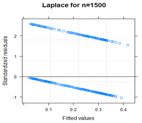
Figure 2. Standard residuals versus fitted values of glmmPQL for health data
Table 3 indicates corresponding model coefficients for glmmLA with model performance metric parameters.
Figure 3 shows points in the residual plot which are not randomly dispersed around the horizontal axis, this indicates glmmLA might not be appropriate for the data.
Table 4 indicates corresponding model coefficients for glmmGHQ with model performance metric parameters (i.e. AIC, BIC and Deviance).
Figure 4 illustrates that for each predictor; the main effect point and its conditional effect points are not vertically aligned. This might indicate that the glmmLA is not suitable for fitting the clinical data.
Table 3. Coefficient of predictors using Laplace approximation model for health data (glmmLA)
|
|
Coef. |
S. E |
$Z$ |
P-Value |
|
Int. |
-1.4770 |
0.33505 |
-4.408 |
1.04e-08** |
|
Ndiag |
0.0547 |
0.03430 |
1.595 |
0.111 |
|
Bgrp |
-0.4087 |
0.08259 |
-4.948 |
7.49e-07** |
|
Gtype |
-0.1589 |
0.08384 |
-1.895 |
0.058 |
|
Sstat |
0.01472 |
0.16906 |
0.087 |
0.931 |
|
Model Performance |
||||
|
AIC |
BIC |
Null Dev. |
Dev. |
DF |
|
1279.89 |
1345.15 |
836.45 |
729.97 |
1498 |
Figure 3. Standard residuals versus fitted values of Laplace approximation model
Table 4. Predictor coefficients with Gauss-Hermite quadrature (glmmGHQ) model for health data
|
|
Coef. |
S. E |
$Z$-Est. |
P-Value |
|
Int. |
-1.4770 |
0.33505 |
-4.408 |
1.04e-08*** |
|
Ndiag |
0.05471 |
0.03430 |
1.595 |
1.11e-01 |
|
Bgrp |
-0.4086 |
0.08259 |
-4.948 |
7.49e-07** |
|
Gtype |
-0.1589 |
0.08384 |
-1.895 |
5.80e-02 |
|
Sstat |
-0.0147 |
0.16906 |
0.087 |
9.31e-01 |
|
Model Performance |
||||
|
AIC |
BIC |
Null Dev |
Deviance |
D.F |
|
1280.00 |
1325.15 |
835.45 |
729.97 |
1491 |
Figure 4. Standard residuals versus fitted values of glmmLA for health data
Figure 5 shows each predictor's main and conditional effect point, which are almost vertically aligned. This plot indicates the suitability of the proposed model (glmmGHQ).
The correlation coefficients across covariates for the real data can be found in Table A2. High multicollinearity is a result of two or more predictor variables in a regression model being highly correlated. A correlation coefficient of 0.8132 between Age and follow-up indicates a strong positive relationship, using generalized linear mixed models and help to prevent the negative impact of the high correlation between these two variables.
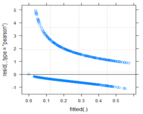
Figure 6 shows points in the residual plot, which are slightly randomly dispersed around the horizontal axis; this shows glmmGHQ being appropriate for the dataset. Table 3 confirmed the model fitness and superiority of glmmGHQ over others and using the corresponding fixed regression coefficients of glmmGHQ, it is observed that the number of diagnoses within the period of investigation accounted for increase in clinical follow-up of individual patients. Using the regression coefficients, for every increase in follow-up status, there is a corresponding increase in number of medical diagnoses by a factor of 0.05471.
Figure 5. Standardized effect sizes of model R squared for glmmGHQ model
Figure 6. Standard residuals versus fitted values of glmmGHQ for health data
The results in Table 4 also shows that for every unit increase in follow-up of patients, there is a decrease in rate of smoking by 0.01473.
The effects of adequate follow-up attributes have been clearly shown in the table with a reduction in the number of individual patients smoking during the period. The age factor effects have also been shown with an increase in the number of diagnoses among older patients. The study tends to influence a positive change of attitudes towards medical appointments. Medical ailments that may be deadly will be discovered early enough due to prompt medical follow-up attitudes.
Figure 5 shows residuals versus fitted values of glmmGHQ approximation model. The points in the residual plot are slightly randomly dispersed around the horizontal axis, this might indicate a good fit for the model (glmmGHQ) appropriate for fitting the clinical data. Figure 1 shows points the residual plot, which are randomly dispersed are horizontal axis; this indicates that glmmPQL might not be appropriate for the data. Figure 2 shows points in the residual plot are not randomly dispersed around the horizontal axis; glmmLA might not be appropriate for the data.
Figure 6 shows violation of normality assumptions on the plot since the points forming a line are not roughly straight. Figure 6 shows that for each predictor, the main effect point and its conditional effect points are almost vertically aligned. This plot indicates the suitability of the model glmmGHQ.
Dependent variables (follow-up status) of 1500 patients attending the selected hospitals for twelve months were analyzed to justify the choice of generalized linear mixed models for this paper in Table 4. The covariates include sex, age, Range, Ndiag, Bgrp, Gtype and Sstat of patients within the period were also examined. Considering the mean and variance of the binary response variable (0.8470, 0.1506), a clear indication of non-normality suspected which justifies the option for fitting the clinical data with generalized linear mixed models in this paper. Table 5 shows the combined estimations based on the underlying models, and Table 6 shows the model performance.
Table 5. Summary of model
|
Models |
Variables |
Regression Cofficients |
Standard Errors |
|
glmmPQL |
Intercept |
-1.47770 |
0.335057 |
|
Sex |
0.14495 |
0.143100 |
|
|
Age |
0.05411 |
0.004341 |
|
|
Ndiag. |
0.01257 |
0.034307 |
|
|
Bgrp |
-0.40868 |
0.082594 |
|
|
Gtype |
-0.15890 |
0.083840 |
|
|
Sstat |
0.014729 |
0.169060 |
|
|
glmmLA |
Intercept |
-1.47706 |
0.335058 |
|
Sex |
0.14396 |
0.143100 |
|
|
Age |
0.03497 |
0.004341 |
|
|
Ndiag. |
0.05471 |
0.034307 |
|
|
Bgrp |
-0.40869 |
0.082594 |
|
|
Gtype |
-0.15891 |
0.083840 |
|
|
Sstat |
0.01472 |
0.169060 |
|
|
glmmAGH |
Intercept |
-1.47706 |
0.335057 |
|
Sex |
0.14496 |
0.143100 |
|
|
Age |
0.03497 |
0.004341 |
|
|
Ndiag. |
0.05471 |
0.034307 |
|
|
Bgrp |
-0.40869 |
0.082594 |
|
|
Gtype |
-0.15890 |
0.083840 |
|
|
Sstat |
-0.01473 |
0.169069 |
Table 6 shows that the glmmGHQ outperformed the two other models. Model fitness and suitability of glmmGHQ is better in terms of model performance metrics (AIC, BIC and Deviance). Comparing all models in this study with the glmmGHQ, it is obvious from the table using AIC, BIC and Deviance values that glmmGHQ fits better than all other models with minimum AIC and BIC of 1275.13 and 1325.20 respectively in Table 6. This discovery may support a choice of glmmGHQ for data analysis involving binary responses subsequently. Researchers may adopt glmmGHQ in fitting data with binary response.
Table 6. Model performance
|
|
AIC |
BIC |
|
glmmPQL |
1277.9 |
1335.15.0 |
|
glmmLA |
1279.89.0 |
1345.15 |
|
glmmGHQ |
1275.13** |
1361.2** |
Appropriate modeling for medical data with binary response has some obvious and important implications for patient diagnoses in Health care system. In this paper, the observation of multiple correlation across covariates is an indication of the presence of random effects because of repeated measures on predictor variables. This made it extremely difficult to model such data using traditional generalized linear model, which does not accommodate random effects. The choice of GLMMs was to take care of multi-collinearity effects across covariates to avoid model misspecification.
The statistical inference drawn from this study shows the fitness and superiority of a gauss-Hermite quadrature estimation technique over other estimation techniques based on some selected model performance metrics for the real data set.
In addition, the study was not only meant to establish the fitness or superiority of the model (glmmGHQ) over others but to also validate effects of clinical follow-up on Patient's medical diagnoses over a period of twelve months leveraging on the fitness of the model (glmmGHQ). Table 4 shows increase in medical diagnoses for more follow-up status of individuals. Using the statistics, for every unit increase in follow-up status, there is a corresponding increase of 0.05471 of number of diagnoses. It is also an observation from Table 4 that with a unit increase in the follow-up status, there is a decrease of 0.01473 in smoking habit of patients. The follow-up effects also trigger an increase of 0.03497 factor in older individual patients. Older patients tend to have more diagnoses than other age categories according to the study results.
Leveraging research results, patients with prompt response to clinical follow-up had a corresponding increasing number of diagnoses, which helped in early detection of ailments that could have been deadly. The result analysis showed patients with follow-up status with a decrease in smoking attributes, which might be a result of clinical counselling during medical appointments.
Based on the research results, the gauss-hermite Quadrature technique might be preferred in estimating model parameters for generalized linear mixed models with binary responses better model results. Investigating effects of risk factors in health care systems may also be carried out using a gauss-Hermite Quadrature technique.
All authors acknowledge the funding sponsor, Covenant University Centre for Research, Innovation and Discovery (CUCRID), Covenant University for their support.
Table A1. Descriptive statistics
|
Desc.Stat. |
Followup |
Sex |
Age |
Ndiagnosis |
Bgroup |
|
Mean |
0.184667 |
0.460000 |
30.02067 |
2.681333 |
1.656000 |
|
Standard Error |
0.010022 |
0.012873 |
0.471299 |
0.051015 |
0.022952 |
|
Median |
0.000000 |
0.000000 |
35.00000 |
2.000000 |
1.000000 |
|
Mode |
0.000000 |
0.000000 |
37.00000 |
1.000000 |
1.000000 |
|
Std Dev. |
0.388156 |
0.498564 |
18.25332 |
1.975784 |
0.790100 |
|
Variance |
0.150665 |
0.248566 |
333.1837 |
3.903721 |
0.888900 |
|
Kurtosis |
0.647809 |
-1.97680 |
-1.36130 |
4.242080 |
0.824400 |
|
Skewness |
1.626944 |
0.160675 |
-0.12010 |
1.748514 |
1.297400 |
|
Range |
1.000000 |
1.000000 |
77.00000 |
14.00000 |
3.000000 |
|
Minimum |
0.000000 |
0.000000 |
0.000000 |
1.000000 |
1.000000 |
|
Maximum |
1.000000 |
1.000000 |
77.00000 |
15.00000 |
4.000000 |
|
Sum |
277.0000 |
690.0000 |
45031.00 |
4022.000 |
2484.300 |
|
Count |
1500.000 |
1500.000 |
1500.000 |
1500.000 |
1500.000 |
Table A2. Correlation matrix of variables
|
Variable |
Followup |
Sex |
Age |
Ndiagnosis |
Bgroup |
Gnotype |
Status |
|
Follouwup |
1.0000 |
-0.025 |
0.8132** |
0.0174 |
- |
-0.0187 |
0.0027 |
|
Sex |
-0.0255 |
1.000 |
-0.0237 |
-0.0003 |
- |
-0.0470 |
0.0480 |
|
Age |
0.8132** |
-0.023 |
1.0000 |
0.6318* |
- |
0.0821 |
0.0093 |
|
Ndiagnosis |
0.0174 |
-0.000 |
0.6318* |
1.0000 |
- |
0.0455 |
-0.0202 |
|
Bgroup |
- |
- |
- |
- |
1.0000 |
- |
- |
[1] Bolker, B.M., Brooks, M.E., Clark, C.J., Geange, S.W., Poulsen, J.R., Stevens, M.H.H., White, J.S.S. (2009). Generalized linear mixed models: A practical guide for ecology and evolution. Trends in Ecology & Evolution, 24(3): 127-135. https://doi.org/10.1016/j.tree.2008.10.008
[2] Gelman, A., Hill, J. (2007). Data analysis using regression and multilevel/hierarchical models. Cambridge University Press.
[3] Vaida, F., Blanchard, S. (2005). Conditional akaike information for mixed-effects models. Biometrika, 92(2): 351-370.
[4] Snijders, T.A.B., Bosker, R.J. (1999). Multilevel analysis: An introduction to basic and advanced multi-level modeling. Sage Publications, London.
[5] Lee, Y., Nelder, J.A., Pawitan, Y. (2006) Generalized linear models with random effects. Chapman and Hall/CRC, Boca Raton.
[6] Breslow, N.E. (1984). Extra-poisson variation in log-linear models. Applied Statistics, 33: 38-44. https://doi.org/10.2307/2347661
[7] Adesina, O.S., Agunbiade, D.A., Oguntunde, P.E (2021). Flexible bayesian mixture models for count data. Scientific African, 13: 1-12. https://doi.org/10.1016/j.sciaf.2021.e00963
[8] Breslow, N.E., Clayton, D.G. (1993). Approximate inference in generalized linear mixed models. Journal of the American Statistical Association, 88: 9-25. https://doi.org/10.1080/01621459.1993.10594284
[9] Bates, D., Mächler, M., Bolker, B., Walker, S. (2015). Fitting linear mixed-effects models using lme4. Journal of Statistical Software, 67(1): 1-48. https://doi.org/10.18637/jss.v067.i01
[10] Adesina, O.S., Adekeye, K.S., Adedotun, A.F., Adeboye, N.O., Ogundile, P.O., Odetunmibi, O.A. (2023). On the performance of dirichlet prior mixture of generalized linear mixed models for zero truncated count data. Journal of Statistics Applications & Probability, 12(3): 1169-1178.
[11] Casals, M., Girabent-Farres, M., Carrasco, J.L. (2014). Methodological quality and reporting of generalized linear mixed models in clinical medicine (2000–2012): A systematic review. PloS one, 9(11): e112653. https://doi.org/10.1371/journal.pone.0112653
[12] Casals, M., Martinez, A.J. (2013). Modelling player performance in basketball through mixed models. International Journal of Performance Analysis in Sport, 13(1): 64-82. https://doi.org/10.1080/24748668.2013.11868632
[13] Fong, Y., Rue, H., Wakefield, J. (2010). Bayesian inference for generalized linear mixed models. Biostatistics, 11(3): 397-412. https://doi.org/10.1093/biostatistics/kxp053
[14] Zhao, Y., Staudenmayer, J., Coull, B.A., Wand, M.P. (2006). General design Bayesian generalized linear mixed models. Statistical Science, 21(1): 35-51. https://www.jstor.org/stable/27645735.
[15] Zhou, M., Carin, L. (2013). Negative binomial process count and mixture modeling. IEEE Transactions on Pattern Analysis and Machine Intelligence, 37(2): 307-320. https://doi.org/10.1109/TPAMI.2013.211
[16] Adesina, O.S., Okewole, D.M., Adedotun, A.F., Adekeye, K.S., Edeki, O.S., Akinlabi, G.O. (2023). Regularized models for fitting zero-inflated and zero-truncated count data: A comparative analysis. Mathematical Modelling of Engineering Problems, 10(4): 1135-1141. https://doi.org/10.18280/mmep.100405
[17] Dare, R.J., Adesina, O.S., Oguntunde, P.E., Agboola, O.O. (2019). Adaptive regression model for highly skewed count data. International Journal of Mechanical Engineering & Technology, 10(1): 1964-2197.
[18] Hasan, F.M., Hussein, T.F., Saleem, H.D., Qasim, O.S. (2024). Enhanced unsupervised feature selection method using crow search algorithm and Calinski-Harabasz. International Journal of Computational Methods and Experimental Measurements, 12(2): 185-190. https://doi.org/10.18280/ijcmem.120208
[19] Deshmukh, M., Bhairnallykar, S., Bukkawar, S., Sharma, R., Kale, S. (2024). Machine learning approach combined with statistical features in the classification of peripheral pulse morphology. International Journal of Computational Methods and Experimental Measurements, 12(1): 69-75. https://doi.org/10.18280/ijcmem.120108
[20] Nelder, J.A., Wedderburn, R.W.M. (1972). Generalized linear models. Journal of the Royal Statistical Society, A, 135(3): 370-384.