Machine Learning for Markov Modeling of COVID-19 Dynamics Concerning Air Quality Index, PM-2.5, NO2, PM-10, and O3

Izaz Ullah Khan![]() | Mehran Ullah*
| Mehran Ullah*![]() | Seema Tripathi | Motiram Sahu
| Seema Tripathi | Motiram Sahu![]() | Anwar Zeb
| Anwar Zeb![]() | Faiza
| Faiza![]() | Anil Kumar
| Anil Kumar![]()
© 2024 The authors. This article is published by IIETA and is licensed under the CC BY 4.0 license (http://creativecommons.org/licenses/by/4.0/).
OPEN ACCESS
In this research Python machine learning module sklearn has been utilized to solve the Markov model. Markov modelling of the COVID-19 dynamics with air quality index (AQI), PM-2.5, NO2, PM-10, and O3, respectively. Data of the Chhattisgarh state of India has been analyzed in two phases. In phase-1 the time duration is from March 15, 2020, to May 01, 2020, and for phase-2 it is from Jun 01, 2020, to Jul 15, 2020. It has been noticed that initially change in AQI from 103 to 84.83 changed disease dynamics, and the first cases of COVID-19 reported. In the next two fortnights March 15, 2020, and April 01, 2020, the dynamics are the same, later the AQI change from 84.83 to 63.83, but no change reported disease dynamics from April 15, 2020, to Jul 15, 2020. In phase 1, a cyclic trend has been observed for changes concerning PM-2.5. The trends for PM-2.5, NO2, PM-10, and O3, respectively are same, but for O3 it is different. COVID-19 reports a negative correlation with AQI, PM-2.5, NO2, PM-10. Moreover, a positive correlation with O3. This proves that the lockdown and ban on transport activities improved AQI, PM-2.5, NO2, PM-10, but not O3.
novel corona virus, AQI, PM-2.5, NO2, PM-10, O3, eigen space decomposition, COVID-19
Novel corona virus initially originated from Wuhan City, Hubei Province, of China. The first case reported by the World Health Organization was on 31 December 2019. The corona virus pandemic has reported a huge number of losses in terms of life and economic sabotage. All the nations of the World have fulfilled their corporate social responsibility by implementing strict safety measures to reduce its effects. Scientists around the world are striving untiringly to investigate the true nature and the remedy of the COVID-19 virus. The most dangerous effect of corona virus infection is its presence without symptoms at the initial stages and thereafter requiring a long duration of isolation [1] and now Cytokine’s storm caused by the virus is the most serious challenge before the scientific world which is the main reason for organs dysfunctions and mortality.
Machine learning is a field of study concerning the development of statistical based learning algorithms. Machine learning models learn from data and then generalize the unseen data so that no explicit instructions are required. Different techniques of machine learning have been adopted to model the disease spreads, disease diagnostics and suggesting medications for various diseases. Uncertainty in system modeling is an important aspect to address. Many authors in the World tried to model uncertainty in the modeling process. Khan et al. [2-4] incorporated uncertainty in system modeling. Khan and Rafique [5] used fuzzy uncertain information to model the aviation network of US airline. Khan and Karam [6] used DEA models to address the performance of the US Airlines. In the research [7], adoptive techniques were adopted to solve linear programming models. Machine leaning approach was adopted in the study [8] to address the adsorption removal in textile wastewater. In the study [9], machine learning approach was adopted to delay problem in aviation network. Thus, it is clear that the machine learning techniques have positively used in the literature for system modeling.
A positive correlation between the air pollution index and COVID-19 cases has been reported from different parts of the world [10]. It is believed that the air pollution is one of the major contributors for unnatural death across the world and about 8% of total death, especially in Asia, Africa, and Europe occurs due to air pollution, and nearly 91% population of the world are living in a polluted environment (WHO, 2016). Air pollution-induced cardiovascular failure, respiratory failure, and finally death has been reported [11, 12]. The primary target of COVID-19 is the lungs which cause potential alveolar damage which leads to asphyxia and finally death [13].
In this study changes in air quality due to lockdown using machine learning in Buenos Aires, Argentina is reported. Lovrić et al. [14] used machine learning techniques to compare the concentrations recorded in the normal situations and lockdown for PM1, PM2.5, and PM10, in Zargeb, Croatia. Mehmood et al. [15] presented the advantages of using machine learning techniques for predicting air quality. Kazi et al. [16] studied the relationship among PM2.5, PM10, SO2, NO2, NO and CO using linear regression model in R language. Méndez et al. [17] proposed a survey of the machine learning approaches for predicting air quality. Islam et al. [18] used machine learning approaches for predicting PM2.5 in Dhaka, Bangladesh. Zukaib et al. [19] studied the impact of air quality on the cases of COVID-19.
It has been also reported that the serious damage of cardiac tissue at both histological and physiological levels is being caused by the COVID-19 virus up to a fatal level. Thus, there is sufficient evidence that air pollutants accelerate present pandemic and lethality. There is no doubt that human is the main contributor in air pollution and with the suspension of human activities during lockdown period the air quality improvement was expected and reported, but the impact of improved air quality and dynamics of COVID-19 pathogenicity has not been studied properly.
Now it is a serious challenge before us to plan a methodology to stop the transmission of virus because still we do not have any effective tool to protect the population. In this condition, the mathematical modeling may be helpful to understand the transmission dynamics of SARS-CoV-2 and will be helpful for future planning. As per the report of WHO, 2002, around 26% of worldwide mortality in 2001 was caused by infectious disease. In recent past sudden increase in infectious disease viz. SARS-CoV in 2003, Mers-CoV in 2012, Ebola in 2014, and SARS-CoV-2 in 2019 have posed a serious threat before human civilization and thus prediction and understanding about the dynamics of the epidemic is nowadays an urgent need of the hour. A proper understanding of disease dynamics may be helpful for its effective control and elimination. The SIR (Susceptibility, infected, and recovered) model may be extremely helpful for the protection of human life. In India, four major epidemiology models are being practiced. The first model is developed by the Indian Council of Medical Research (ICMR); the second model by the University of Michigan; the third by John Hopkins University and the fourth one is the model proposed by Cambridge University. Some objections have been raised about the above models with the arguments that the above models have not considered larger population size and population driving factors.
A review of the literature depicts that Markov model of the COVID-19 dynamics have never been addressed with the help of machine learning approach. In this study machine learning technique is adopted for Markov modelling of the COVID-19 dynamics with variations in AQI, PM-2.5, NO2, PM-10, and O3, respectively. The long-run dynamics of the novel corona virus infection dynamics are investigated related to changes in AQI, PM-2.5, NO2, PM-10, and O3, respectively, in the Chhattisgarh state of India. The present study is an attempt to addresses the following objectives.
(1) To formulate the Markov model of the long-run dynamics of the novel corona virus infections concerning changes in AQI (PM-2.5, NO2, PM-10, and O3) the Chhattisgarh state of India.
(2) To solve the formulate model in step 1 using Machine learning techniques.
(3) To address the initial dynamics of the novel corona virus infections related to changes in PM-2.5, NO2, PM-10, and O3 levels in the Chhattisgarh state of India based on the initial transition matrix.
The study is supposed to answer the following hypothesis.
(1) There is a direct relation between AQI and the cases of COVID-19 cases.
(2) PM-2.5 level and the cases of COVID-19 cases are positively related.
(3) There is positive relation between NO2 level and COVID-19 cases.
(4) PM-10 level and COVID-19 cases have a direct relation.
(5) O3 level and COVID-19 cases are directly related.
In the present study, the Markov process is elaborated in Section 2. In Section 3, the Markov process is implemented for addressing the long-run disease dynamics concerning changes in AQI levels. In Section 4, the proposed machine learning for Markov model of the long-run disease dynamics concerning changes in PM-2.5, NO2, PM-10, and O3 levels, respectively is presented. In Section 5, the results obtained for addressing the long-run disease dynamics concerning changes in AQI levels analyzed and discussed. In Section 6, the results obtained for the disease dynamics concerning changes in PM-2.5, NO2, PM-10, and O3 levels, respectively are analyzed. Correlation of COVID-19 Infections concerning PM-2.5, NO2, PM-10 and O3 is presented in Section 7. Finally, the findings have been concluded in Section 8.
Markov chain is a process where the future state of a system can be predicted based on its current state. A transition matrix is an n*n two dimensions array of elements having n rows and n columns and it is denoted as T=[tij],1≤i≤n,1≤j≤n. The column matrix “u” given in (1) is called the long-run vector.
u=[u1u2⋅⋅⋅un],1≤i≤n (1)
One of the characteristic properties of the transition matrix is to determine the system states at future times by knowing the current state. Assume if x(k) denote the state vector at any time “k”, where x(0) is the initial state, denoted as (2).
x(k)=[p(k)1p(k)2⋅⋅⋅p(k)n],0≤k (2)
Theorem (1) helps to identify the future state of Markov’s Process.
Theorem 1: If “T” is the transition matrix of a Markov process, the future state x(k+1) can be found from the knowing of the state x(k) as in (3).
x(k+1)=Tx(k) (3)
Proof:
From Eq. (3), we can find (4).
x(1)=Tx(0) (4)
x(2)=Tx(1) (5)
Put Eq. (4) in Eq. (5).
x(2)=Tx(1)=TT(x)0=T2(x)0 (6)
x(3)=Tx(2)=TT2(x)0=T3(x)0 (7)
Continuing in this way, we finally get Eq. (8).
x(n)=Tnx(0) (8)
This completes the proof.
Definition 1: Given a transition matrix “T”, as n→∞,Tn approaches (9) [20].
A=[u1u1⋅⋅⋅u1u2u2⋅⋅⋅u2⋅⋅⋅⋅⋅⋅⋅⋅⋅ununun] (9)
Theorem 2: Given “T” is the transition matrix and “A” and “u” satisfy Definition 1, then (a) and (b) holds.
(a) For a transition matrix “x”, Tnx→u as n→∞, “u” is called the steady-state vector.
(b) The steady-state vector “u” is uniquely satisfying Tu=u.
Proof:
(a) Let consider the matrix (10).
x=[x1x2⋅⋅xn] (10)
We know from Definition 1 , that as n→∞,Tn→A, giving Tnx→Ax. Using (9) and (10) we can construct (11).
Ax=[u1u1⋅⋅⋅u1u2u2⋅⋅⋅u2⋅⋅⋅⋅⋅⋅⋅⋅⋅ununun]⋅[x1x2⋅⋅⋅xn] (11)
Ax=[u1x1+u1x2+.⋅⋅+u1xnu2x1+u2x2+...+u2xn⋅.⋅⋅⋅.unx1+unx2+...+unxn] (12)
Also, (x1+x2+.⋅⋅+xn)=1 thus (12) can be written as (13).
Ax=[u1(x1+x2+⋅⋅⋅+xn)u2(x1+x2+⋅⋅⋅+xn)⋅⋅⋅⋅⋅⋅un(x1+x2+⋅⋅⋅+xn)]=[u1u2⋅⋅un] (13)
Eq. (13) proves Tnx→u.
(b) We have Tn→A as n→∞, which means Tn+1→A. Knowing Tn+1=Tn⋅T. Thus Tn+1→A, so TA=A. Thus we can write Tu=u.
Moreover, it is required that “u” is unique. Suppose “v” is another matrix such that Tv=v. From part (a) we know, Tnv→u. Moreover, Tv=v implying Tnv=u,∀n, so u=v.
If the transition matrix T=[tij],1≤i≤n,1≤j≤n, of a Markov process, then for variables " x ", when n→∞,Tnx→ u, where, u denotes steady-state vector. Note that the steadystate vector satisfies (14).
Tu=u (14)
Tu=Inu (15)
Inu−Tu=0 (16)
(In−T)u=0 (17)
The modeled Eq. (17) is referred to as the eigen space of the transition matrix “T”. Solving (17), we can determine the eigen space decomposition of the matrix “T”. Python machine learning module sklearn is adopted to solve the Markov model (17).
This section is dedicated to studying the effects of the air quality index on the COVID-19 dynamics in the Chhattisgarh state of India. The fortnightly data of the AQI level and disease confirmed cases are shown in Table 1.
From the data given in Table 1 the transition matrix of the corona virus infection (Tex translation failed) concerning the air quality index AQI can be formulated as in Eq. (18).
The transition matrix TAQI in show the matrix of average change in the cases of COVID-19 with average change in the AQI level spanned over different fortnights. It is worth noting that matrix (18) is not the probabilities, it the matrix showing the change in the COVID-19 with respect to change in AQI. Eq. (19) models the eigen space decomposition of the COVID-19 concerning the air quality index in the Chhattisgarh state of India.
Solving Eq. (21) with help of Python machine learning module sklearn we get the eigen values as shown in the program run file given below. The gradient decent optimizer of the Python machine learning module sklearn is utilized to report the following solution for the Markov’s model developed in (21).
Table 1. Average air quality index of the Chhattisgarh state and cases of corona virus infections
|
Month |
Average Air Quality Index of the Chhattisgarh State (µg/m3) |
Cases of Corona Virus Infections |
|
Mar-01 |
103 |
0 |
|
Mar-15 |
84.83 |
1 |
|
Apr-01 |
63.83 |
8 |
|
Apr-15 |
64.61 |
33 |
|
May-01 |
101.05 |
40 |
|
May-15 |
67.16 |
60 |
|
Jun-01 |
56.16 |
498 |
|
Jun-15 |
35.83 |
1715 |
|
Jul-01 |
43.66 |
2660 |
|
Jul-15 |
29.33 |
4379 |
|
Jul-20 |
|
5407 |
TAQI =[ State 10384.8363.8364.61101.0567.1656.1635.8343.6629.331031−0.055−0.025−0.0260−0.5128−0.0278−0.0213−0.01488−0.0168−0.213584.830.38521−0.3333−0.34610.4315−0.3961−0.2441−0.1428−0.1700−0.126163.830.63821.189132.050.67167.50−3.25−0.8928−1.23−0.724664.610.18230.3461−8.9710.19202.745−0.8284−0.2432−0.3341−0.1984101.0510.25−1.233−0.5373−0.54881−0.590−0.4455−0.3066−0.3484−0.278867.1612.2224.787−131.53−171.7612.921−39.81−13.98−18.63−11.5756.1625.9842.44158.67144.0227.11110.31−59.86−97.36−45.3535.8314.0619.2833.7532.8314.4830.1646.481120.68−145.3843.6628.9841.7585.2282.0529.9573.14137.52−219.541−119.9529.3313.9518.5229.7929.1314.3327.1738.31158.1571.731] (18)
(λIn−TAQI)u=0 (19)
(λ[1000000000010000000000100000000001000000000010000000000100000000001000000000010000000000100000000001]−[1−0.055−0.025−0.0260−0.5128−0.0278−0.0213−0.01488−0.0168−0.21350.38521−0.3333−0.34610.4315−0.3961−0.2441−0.1428−0.1700−0.12610.63821.189132.050.67167.50−3.25−0.8928−1.23−0.72460.18230.3461−8.9710.19202.745−0.8284−0.2432−0.3341−0.198410.25−1.233−0.5373−0.54881−0.590−0.4455−0.3066−0.3484−0.278812.2224.787−131.53−171.7612.921−39.81−13.98−18.63−11.5725.9842.44158.67144.0227.11110.31−59.86−97.36−45.3514.0619.2833.7532.8314.4830.1646.481120.68−145.3828.9841.7585.2282.0529.9573.14137.52−219.541−119.9513.9518.5229.7929.1314.3327.1738.31158.1571.731]).[u1u2u3u4u5u6u7u8u9u10]=[0000000000] (20)
([λ−10.0550.0250.02600.51280.02780.02130.014880.01680.2135−0.3852λ−10.33330.3461−0.43150.39610.24410.14280.17000.1261−0.6382−1.189λ−1−32.05−0.6716−7.503.250.89281.230.7246−0.1823−0.34618.97λ−1−0.1920−2.7450.82840.24320.33410.1984−10.251.2330.53730.5488λ−10.5900.44550.30660.34840.2788−12.22−24.787131.53171.76−12.92λ−139.8113.9818.6311.57−25.98−42.44−158.67−144.02−27.11−110.3λ−159.8697.3645.35−14.06−19.28−33.75−32.83−14.48−30.16−46.48λ−1−120.68145.38−28.98−41.75−85.22−82.05−29.95−73.14−137.52219.54λ−1119.95−13.95−18.52−29.79−29.13−14.33−27.17−38.31−158.15−71.73λ−1]).[u1u2u3u4u5u6u7u8u9u10]=[0000000000] (21)
runfile('C:/Users/Ehsan/.spyder-py3/temp.py', wdir='C:/Users/Toshiba/.spyder-py3')
[0.25137211+269.603379j 0.25137211-269.603379j
1.20795455+104.37879212j 1.20795455-104.37879212j
1.41174851+32.71252034j 1.41174851-32.71252034j
1.62399294+3.23631201j 1.62399294-3.23631201j
0.50493189+1.20088642j 0.50493189-1.20088642j]
The corresponding eigen space is give below in python program runfile.
runfile('C:/Users/Ehsan/.spyder-py3/temp.py', wdir='C:/Users/Toshiba/.spyder-py3')
[0.25137211+269.603379j 0.25137211-269.603379j
[9.32594206e-05-4.33783496e-05j 9.32594206e-05+4.33783496e-05j
5.15105486e-04-6.16206590e-04j 5.15105486e-04+6.16206590e-04j
-2.95210718e-03+4.97001251e-03j -2.95210718e-03-4.97001251e-03j
-5.46487389e-02+6.53587008e-02j -5.46487389e-02-6.53587008e-02j
8.48866277e-02+1.60693406e-03j 8.48866277e-02-1.60693406e-03j]
[4.77093239e-05+6.23698503e-04j 4.77093239e-05-6.23698503e-04j
8.25279752e-04-2.02434977e-03j 8.25279752e-04+2.02434977e-03j
-3.61688735e-03+6.28184619e-03j -3.61688735e-03-6.28184619e-03j
6.05143864e-02+5.96991228e-02j 6.05143864e-02-5.96991228e-02j
5.11313568e-02+2.44398974e-01j 5.11313568e-02-2.44398974e-01j]
[1.75794669e-03+5.66361516e-03j 1.75794669e-03-5.66361516e-03j
-2.91305369e-02-1.83967222e-02j -2.91305369e-02+1.83967222e-02j
-8.93964292e-03-1.45665309e-01j -8.93964292e-03+1.45665309e-01j
1.47439956e-01-8.00542150e-03j 1.47439956e-01+8.00542150e-03j
1.39866167e-01-2.77316566e-04j 1.39866167e-01+2.77316566e-04j]
[5.02757782e-04+1.58039634e-03j 5.02757782e-04-1.58039634e-03j
-7.88965875e-03-7.71389291e-03j -7.88965875e-03+7.71389291e-03j
5.23782798e-02-3.51401601e-02j 5.23782798e-02+3.51401601e-02j
-9.66502337e-02+4.24311422e-02j -9.66502337e-02-4.24311422e-02j
-1.14377611e-01+1.69986941e-02j -1.14377611e-01-1.69986941e-02j]
[2.63939859e-04+1.23137334e-03j 2.63939859e-04-1.23137334e-03j
9.14892894e-04-3.78954396e-03j 9.14892894e-04+3.78954396e-03j
-5.86746773e-03+1.05177189e-02j -5.86746773e-03-1.05177189e-02j
1.50977618e-01+3.45604122e-01j 1.50977618e-01-3.45604122e-01j
-2.82296530e-01-1.87691619e-01j -2.82296530e-01+1.87691619e-01j]
[-3.00539422e-03+7.96984546e-02j -3.00539422e-03-7.96984546e-02j
-1.60952084e-02-3.24995953e-01j -1.60952084e-02+3.24995953e-01j
3.82300573e-01+2.36400816e-01j 3.82300573e-01-2.36400816e-01j
3.76387989e-01-1.71265407e-01j 3.76387989e-01+1.71265407e-01j
4.66110948e-01-7.05657507e-02j 4.66110948e-01+7.05657507e-02j]
[1.97441548e-01+2.58104409e-01j 1.97441548e-01-2.58104409e-01j
-6.55321573e-01+0.00000000e+00j -6.55321573e-01-0.00000000e+00j
-3.00486585e-01+2.72072492e-01j -3.00486585e-01-2.72072492e-01j
-3.08052737e-01-1.85951023e-02j -3.08052737e-01+1.85951023e-02j
-2.73133553e-01+2.76245203e-03j -2.73133553e-01-2.76245203e-03j]
[2.40476322e-01-4.55764974e-01j 2.40476322e-01+4.55764974e-01j
-8.07288211e-02-3.29823300e-01j -8.07288211e-02+3.29823300e-01j
-2.79939180e-01+1.90652195e-02j -2.79939180e-01-1.90652195e-02j
-2.53791134e-01-7.19302442e-03j -2.53791134e-01+7.19302442e-03j
-2.36739698e-01-2.09770937e-04j -2.36739698e-01+2.09770937e-04j]
[6.72441831e-01+0.00000000e+00j 6.72441831e-01-0.00000000e+00j
1.35297091e-01+3.60492639e-01j 1.35297091e-01-3.60492639e-01j
5.47825474e-01+0.00000000e+00j 5.47825474e-01-0.00000000e+00j
5.27347068e-01+0.00000000e+00j 5.27347068e-01-0.00000000e+00j
5.03337385e-01+0.00000000e+00j 5.03337385e-01-0.00000000e+00j]
[-2.22706975e-01-3.47377578e-01j -2.22706975e-01+3.47377578e-01j
-3.45526665e-01+2.83537188e-01j -3.45526665e-01-2.83537188e-01j
4.51477148e-01+1.59574064e-01j 4.51477148e-01-1.59574064e-01j
4.48455654e-01+2.05894360e-02j 4.48455654e-01-2.05894360e-02j
4.19900200e-01+5.84583950e-03j 4.19900200e-01-5.84583950e-03j]]
These results are further discussed and analyzed in section 5.
This study was conducted in two phases. In phase-1, the disease dynamics concerning PM-2.5, NO2, PM-10, and O3, respectively were studied from March 15, 2020, to May 01, 2020, in the state of Chhattisgarh. In phase-2, Corona dynamics concerning PM-2.5, NO2, PM-10, and O3, respectively were studied from June 1, 2020, to July 15, 2020, in the state of Chhattisgarh. The levels of PM-2.5, NO2, PM-10 and O3, in phase-1 are in Table 2.
Table 2. Average level of PM-2.5, NO2, PM-10, O3 for Chhattisgarh state and cases of corona virus infections
|
Time |
Average Level of PM-2.5 |
Average Level of NO2 |
Average Level of PM-10 |
Average Level of O3 |
Cases of Corona Virus Infections |
|
Mar-15 |
102 |
47 |
95 |
4 |
1 |
|
Apr-01 |
61 |
58 |
47 |
4.5 |
8 |
|
Apr-15 |
58 |
59 |
49 |
5 |
33 |
|
May-01 |
119 |
64 |
117 |
5.5 |
40 |
|
May-15 |
69 |
57 |
58 |
6 |
60 |
|
Jun-01 |
42 |
42 |
36 |
12 |
498 |
|
Jun-15 |
23 |
34 |
16 |
20 |
1715 |
|
Jun-30 |
29 |
39 |
22 |
7 |
2660 |
|
Jul-15 |
18 |
30 |
14 |
3 |
4379 |
Table 3. Transition matrix for average number of corona virus cases concerning PM-2.5, NO2, PM-10, O3 in phase-1 for Chhattisgarh state
|
Time |
Change in Average COVID Cases w. r. t Change in Average Level of PM2.5 |
Change in Average COVID Cases w. r. t Change in Average Level of NO2 |
Change in Average COVID Cases w. r. t Change in Average Level of PM10 |
Change in Average COVID Cases w. r. t Change in Average Level of O3 |
|
Mar-15 |
-0.5 |
-0.1428 |
-0.5 |
-1 |
|
Apr-01 |
-0.1707 |
0.6363 |
-0.1458 |
14 |
|
Apr-15 |
-8.333 |
25 |
12.5 |
50 |
|
May-01 |
0.1147 |
1.4 |
0.1029 |
14 |
Table 4. Transition matrix for average number of corona virus cases concerning PM-2.5, NO2, PM-10, O3 in phase-2 for Chhattisgarh state
|
Time |
Change in Average COVID Cases w. r. t Change in Average Level of PM2.5 |
Change in Average COVID Cases w. r. t Change in Average Level of NO2 |
Change in Average COVID Cases w. r. t Change in Average Level of PM10 |
Change in Average COVID Cases w. r. t Change in Average Level of O3 |
|
Jun-01 |
-16.22 |
-29.2 |
-19.9 |
73 |
|
Jun-15 |
-64.05 |
-152.12 |
-60.85 |
152.12 |
|
Jun-30 |
157.5 |
189 |
157.5 |
-72 |
|
Jul-15 |
-156.27 |
-191 |
-214.87 |
-429.75 |
The information is given in Table 2 is used to formulate the transition matrix for phase-1 as shown in Table 3 and Eq. (22).
T1=[−0.5−0.1428−0.8−1−0.17070.6363−0.145814−8.3332512.5500.11471.40.102914] (22)
The transition matrix in (22) show the matrix of average change in the cases of COVID-19 with average change in the PM-2.5, NO2, PM-10, O3 spanned over different fortnights. It is worth noting that matrix (22) does not denote the probabilities, it the matrix showing the change in the COVID-19 with respect to change in AQI. The situation is also shown in Table 3. The eigen space for (22) is given as (23).
(λIn−T1)u=0 (23)
(λ[1000010000100001]−[−0.5−0.148−0.8−1−0.17070.636−0.15814−833325125500.11471.40.102914])[u1u2u3u4]=[0000] (24)
Eq. (24) reduces to (25).
([λ+0550.14280.810.1707λ−0.6360.1458−148.333−25λ−125−50−0.1147−1.4−0.1029λ−14])[u1u2u3u4]=[0000] (25)
Python machine learning module sklearn solves the model (25) and the results are presented below. The gradient decent optimizer of the Python software is utilized to report the following solution for the Markov’s model developed in (25).
runfile('C:/Users/Ehsan/untitled0.py', wdir='C:/Users/Toshiba')
[-0.59830406+0.4925565j -0.59830406-0.4925565j 11.1152819 +0.j
16.71762621+0.j]
Furthermore, the eigen space is given in the program run file below.
runfile('C:/Users/Ehsan/untitled0.py', wdir='C:/Users/Toshiba')
[[0.10057133+0.59609944j 0.10057133-0.59609944j-0.04110036+0.j-0.03265455+0.j]
[-0.36931397+0.27075848j-0.36931397-0.27075848j-0.03556054+0.j 0.04164904+0.j]
[0.65039065+0.j 0.65039065-0.j 0.998382+0.j 0.99692292+0.j]
[0.03104194-0.02960238j 0.03104194+0.02960238j-0.01672071+0.j 0.05782493+0.j]]
This completes the results of phase-1. These results are analyzed and discussed later in section 6.
Based on Table 2, we construct the transition matrix of change in corona virus infections concerning PM-2.5, NO2, PM-10, and O3, respectively, given in Table 4 and Eq. (26).
T2=[−16.22−29.2−19.973−64.05−152.12−60.85152.12157.518.9157.5−72−156.27−191−214.87−429.75] (26)
The transition matrix in (26) show the matrix of average change in the cases of COVID-19 with average change in the PM-2.5, NO2, PM-10, O3 spanned over different fortnights. It is worth noting that matrix (26) does not denote the probabilities, it the matrix showing the change in the COVID-19 with respect to change in AQI. The situation is also shown in Table 4. The eigen space for (26) is given as (27).
(λIn−T2)u=0 (27)
(λ[1000010000100001][−1622−292−19913−6105−122−60.8122157.51891575−12−16627−191−21487−29.5])[u1u2u3u4]=[0000] (28)
Eq. (28) further reduces to (29).
([λ+16.2229.219.9−7364.05λ+152.1260.85−15212−157.5−189λ−157.572156.27191214.87λ+429.75]).[u1u2u3u4]=[0000] (29)
Solution of (29) by the sklearn module of the Python is presented in the following run file.
The gradient decent optimizer of the Python module sklearn is utilized to report the following solution for the Markov’s model developed in (29).
runfile('C:/Users/Ehsan/untitled0.py', wdir='C:/Users/Toshiba')
[-414.13840934 115.09774881-6.60203666-134.94730281]
Moreover the eigen space is give in the following run file.
runfile('C:/Users/Ehsan/untitled0.py', wdir='C:/Users/Toshiba')
[[-0.139249-0.0838735 0.69179567-0.02729547]
[0.4223546 0.36495388 0.07238706-0.81164678]
[-0.21091667-0.89334181-0.7145629 0.56998975]
[-0.87048289 0.24842366 0.07469088 0.12488454]]
These results are discussed and analyzed in section 6.
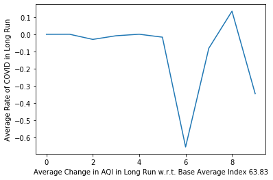
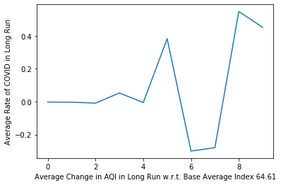
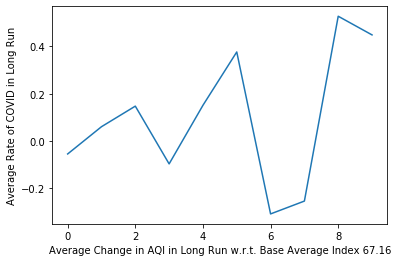
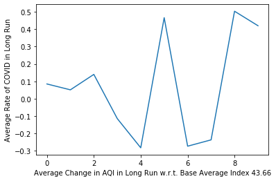
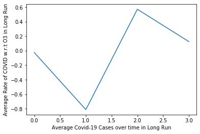
This section is dedicated to discuss and analyze the long-run disease dynamics of the COVID-19 concerning changes in the air quality index. The results obtained in section 3 have been presented through graphical analysis to analyze the disease dynamics in association with the air quality index. The first evidence which is the characteristic property of the eigen space decomposition is the stable and long-run behavior of the disease, this means that the behavior of the disease has not changed. The first case was reported on March 01, 2020, and the long-run behavior of the disease initially is shown in Figure 1. The figure has been drowned and calculated for the period of March 01, 2020, to March 15, 2020, when the AQI has been changed from 103 to 84.83 and the first case has appeared. The graph shows initially a stable behavior, then an increase and then decrease in the Corona infections in the long run for the state of Chhattisgarh. In the next two fortnights March 15, 2020, and April 01, 2020, disease dynamics were found the same as shown in Figure 2 and Figure 3. During this period, the AQI has been changed from 84.83 to 63.83, but without any effect on the disease dynamics in long run. This period has been characterized by a stable, then a decreasing, increasing, and finally a decreasing behavior. In the rest of all fortnights from April 15, 2020, to Jul 15, 2020, the dynamics, in the long run, were found the same as shown in Figures 4-10 which explains that the AQI change does not affect the disease dynamics. The disease dynamics are cyclic with the increasing and decreasing patterns with finally decreasing behavior. The analysis deduces that in long run the disease dynamics change occurs at an AQI 103 to 84.83 and then at 64.61. Changes that occurred in AQI between April 15, 2020, to Jul 15, 2020, did not affect the disease dynamics in long run and in all the cases the long-term dynamics of COVID-19 were finally found moving downward.
Figure 1. Average rate of change corona virus infections with average change in AQI concerning base index 103
Figure 2. Average rate of change corona virus infections with average change in AQI concerning base index 84.83
Figure 3. Average rate of change corona virus infections with average change in AQI concerning base index 63.83
Figure 4. Average rate of change corona virus infections with average change in AQI concerning base index 64.61
Figure 5. Average rate of change corona virus infections with average change in AQI concerning base index 101.05
Figure 6. Average rate of change corona virus infections with average change in AQI concerning base index 67.16
Figure 7. Average rate of change corona virus infections with average change in AQI concerning base index 56.16
Figure 8. Average rate of change corona virus infections with average change in AQI concerning base index 35.83
Figure 9. Average rate of change corona virus infections with average change in AQI concerning base index 43.63
Figure 10. Average rate of change corona virus infections with average change in AQI concerning base index 29.33
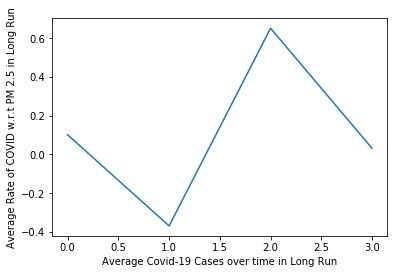
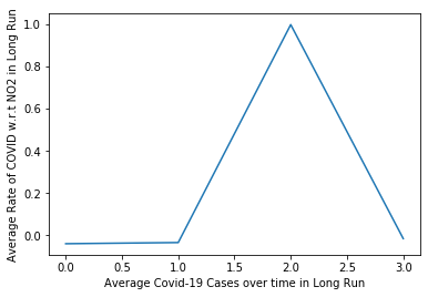
In this section long-run dynamics of COVID-19 Infections concerning PM-2.5, NO2, PM-10, and O3, respectively, have been studied. The study is concluded in two phases. In phase-1 the duration was from March 15, 2020, to May 01, 2020, and in phase-2 the duration was from Jun 01, 2020, to Jul 15, 2020. In phase-1 the solution obtained in section 4 and Figure 11 shows a cyclic trend with initially decreasing, then increasing, and again a decreasing trend. The long-run behavior of NO2 was initially found stable, then become increasing and finally decreasing as shown in Figure 12. The behavior of both PM-10 and O3 was similar with a slight difference from that of NO2, and both are shown in Figures 13 and 14, where initially they do not affect the disease dynamics. This is followed by an increase and finally decreasing behavior of the COVID-19 virus infections which has been depicted.
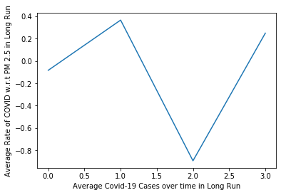
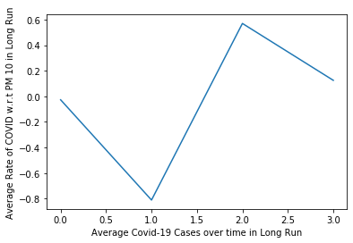
The disease dynamics in phase-2 have been calculated in section 4 and shown in Figures 15-18. Analyzing the figures, we can easily deduce that PM-2.5 and NO2 have a slightly similar effect in long run on the COVID-19 virus infections in the Chhattisgarh State of India as shown in Figures 15 and 16. This trend exhibits from a decreasing to an increasing one. Moreover, in the long run, PM-10 and O3 have similar effects on the COVID-19 virus as shown in Figures 17 and 18. Both of these trends are promising, and they show a behavior from an increasing to a decreasing trend.
Figure 11. Average Rate of change corona virus infections with average change in PM2.5 in phase 1
Figure 12. Average rate of change corona virus infections with average change in NO2 in phase 1
Figure 13. Average rate of change corona virus infections with average change in PM-10 in phase 1
Figure 14. Average rate of change corona virus infections with average change in O3 in phase 1
Figure 15. Average rate of change corona virus infections with average change in PM-2.5 in phase 2
Figure 16. Average rate of change corona virus infections with average change in NO2 in phase 2
Figure 17. Average rate of change corona virus infections with average change in PM-10 in phase 2
Figure 18. Average rate of change corona virus infections with average change in O3 in phase 2
Figure 19. Average rate of change corona virus infections with average change in PM-2.5 based on initial transition
Figure 20. Average rate of change corona virus infections with average change in NO2 based on initial transition
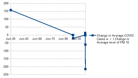
Figure 21. Average rate of change corona virus infections with average change in PM-10 based on initial transition
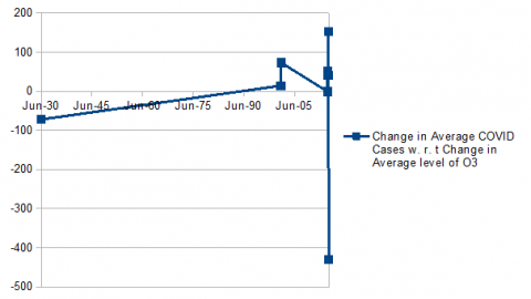
Figure 22. Average rate of change corona virus infections with average change in O3 based on initial transition
Table 5. Initial transition matrix for average number of corona virus cases concerning PM-2.5, NO2, PM-10, O3 for Chhattisgarh state
|
Time |
Change in Average COVID Cases w. r. t Change in Average Level of PM2.5 |
Change in Average COVID Cases w. r. t Change in Average Level of NO2 |
Change in Average COVID Cases w. r. t Change in Average Level of PM10 |
Change in Average COVID Cases w. r. t Change in Average Level of O3 |
|
Mar-15 |
-0.5 |
-0.1428 |
-0.5 |
-1 |
|
Apr-01 |
-0.1707 |
0.6363 |
-0.1458 |
14 |
|
Apr-15 |
-8.333 |
25 |
12.5 |
50 |
|
May-01 |
0.1147 |
1.4 |
0.1029 |
14 |
|
May-15 |
-0.4 |
-2.85 |
-0.338 |
40 |
|
Jun-01 |
-16.22 |
-29.2 |
-19.9 |
73 |
|
Jun-15 |
-64.05 |
-152.12 |
-60.85 |
152.12 |
|
Jun-30 |
157.5 |
189 |
157.5 |
-72 |
|
Jul-15 |
-156.27 |
-191 |
-214.87 |
-429.75 |
Finally, the disease dynamics concerning PM-2.5, NO2, PM-10, and O3, respectively, have been visualized in Figures 19-22 and Table 5. They show that initially, the disease dynamics follow the same trend for PM-2.5, NO2, and PM-10 with only slight changes in the values. In these cases, the rate of disease spread was found decreasing as shown in Figures 19-21. Moreover, for O3 the disease dynamics were found different than the other three parameters, whereby the disease infection rate increases and then decreases as shown in Figure 22. Again, in all the cases, the disease trend was found decreasing.
Several authors have presented some models to combat the problem. The studies [21, 22] have developed model for calculating transmittablility of virus among bats-host-reservoir-people transmission. Lipsitch et al. [23] have established characteristics of epidemiological time distribution. Zhou et al. [10] have proposed statistical model for COVID-19 dynamics for Wuhan. In the present study, the disease dynamics have been modeled as Markov process and solved with the help of machine learning techniques. It has been established that the eigen space decomposition method is suitable for the understanding the long run disease dynamics under influence of the air quality index which is inevitable in near future. In a country like India, it is very difficult to quickly vaccinate the population up to such extend to attain herd immunity when the quantum of the population is 1.35 billion and vaccine production is in the juvenile stage. It is also notable that the half-life of antibody produced after vaccination is not very much stable and is speculated that after one year the next booster dose will be required which may be a herculean task for the system of the country. Thus under such circumstances, the finding of the present study may contribute significantly to the management of dynamics of epidemics along with inevitable seasonal alterations in air quality index and planning of control measures.
This section is dedicated to know the important environmental factors contributing to the virus transmission. Tables 6 and 7 show the correlation between the COVID-19 concerning AQI, PM-2.5, NO2, PM-10 and O3, respectively. It is clear that COVID-19 has negative relation concerning AQI, PM-2.5, NO2, PM-10. Moreover, it has positive relation with ozone O3. This is due to the fact that due to lockdown and ban on transport the air index have improved in all regions of the world as well as in Chhattisgarh state. Although cases of COVID were increasing, the negative effects of -0.77, -0.75, -0.87 and -0.75 were recorded for AQI, PM-2.5, NO2, PM-10, respectively due to lockdown. This showed that due to lockdown AQI, PM-2.5, NO2, PM-10, respectively were improved but the ozone O3 level was not improved in the Chhattisgarh state. This finding agrees with the Sarmadi et al. [24], where they asserted a negative correlation for PM-2.5, NO2, PM-10, respectively. They furthered that the O3 level was not improved in almost all major cities of the world due to COVID-19 lockdown.
Table 6. Correlation of corona virus cases concerning PM-2.5, NO2, PM-10, O3 for Chhattisgarh state
|
RowID |
PM-2.5 |
NO2 |
PM-10 |
O3 |
AQI |
COVID Cases |
|
PM-2.5 |
1.0 |
0.84 |
0.96 |
-0.54 |
0.96 |
-0.75 |
|
NO2 |
0.84 |
1.0 |
0.84 |
-0.45 |
0.83 |
-0.87 |
|
PM-10 |
0.96 |
0.84 |
1.0 |
-0.51 |
0.99 |
-0.75 |
|
O3 |
-0.54 |
-0.45 |
-0.51 |
1.0 |
-0.50 |
0.13 |
|
AQI |
0.96 |
0.83 |
0.99 |
-0.50 |
1.0 |
-0.77 |
|
COVID Cases |
-0.75 |
-0.87 |
-0.75 |
0.13 |
-0.77 |
1.0 |
Table 7. Correlation of corona virus cases concerning PM-2.5, NO2, PM-10, O3
|
First Column Name |
Second Column Name |
Correlation Value |
P Value |
Degrees of Freedom |
|
PM-2.5 |
NO2 |
0.84 |
0.004308801358964498 |
7 |
|
PM-2.5 |
PM-10 |
0.96 |
3.46412906206961E-5 |
7 |
|
PM-2.5 |
O3 |
-0.54 |
0.13026512479868854 |
7 |
|
PM-2.5 |
AQI |
0.96 |
1.8616157591022642E-5 |
7 |
|
PM-2.5 |
COVID Cases |
-0.75 |
0.019512835447252165 |
7 |
|
NO2 |
PM-10 |
0.84 |
0.004189401707549889 |
7 |
|
NO2 |
O3 |
-0.45 |
0.21688487313146854 |
7 |
|
NO2 |
AQI |
0.83 |
0.00489527245350696 |
7 |
|
NO2 |
COVID Cases |
-0.87 |
0.0021296542434908793 |
7 |
|
PM-10 |
O3 |
-0.51 |
0.15260095715429275 |
7 |
|
PM-10 |
AQI |
0.99 |
8.794618144847277E-9 |
7 |
|
PM-10 |
COVID Cases |
-0.75 |
0.01876983678434396 |
7 |
|
O3 |
AQI |
-0.50 |
0.16838793274749242 |
7 |
|
O3 |
COVID Cases |
0.13 |
0.7231742104993175 |
7 |
|
AQI |
COVID Cases |
-0.77 |
0.015127837246095331 |
7 |
Based Tables 6 and 7, we answer the hypothesis as under.
1. There is a direct relation between AQI and the cases of COVID-19 cases.
Reject the null hypothesis as there is negative relation between AQI and the cases of COVID-19.
2. PM-2.5 level and the cases of COVID-19 cases are positively related.
Reject the null hypothesis as there is negative relation between PM-2.5 level and the cases of COVID-19.
3. There is positive relation between NO2 level and COVID-19 cases.
Reject the null hypothesis as there is negative relation between NO2 level and the cases of COVID-19.
4. PM-10 level and COVID-19 cases have a direct relation.
Reject the null hypothesis as there is negative relation between PM-10 level and the cases of COVID-19.
5. O3 level and COVID-19 cases are directly related.
Accept the null hypothesis as there is positive relation between O3 level and the cases of COVID-19. The O3 level was not improved due to COVID-19 lockdown in the Chhattisgarh state as shown in the previous studies.
Finally, we compare our findings with some studies. The main findings of this study are that AQI, PM-2.5, NO2, PM-10 decreased during the lockdown in the Chhattisgarh state. Whereas the level of O3 increased in the Chhattisgarh state during the lockdown. The decrease in NO2 is due to ban on transportation resulting an increase in O3. In normal situations, the concentration of NO3 increases during night. Due to lockdown decrease in NO was reported. This decrease in NO slowed down the degradation of O3 by NO forming NO2. Thus, an access of O3 was present in the atmosphere and at the same time the formation of NO2 was decreased in the lockdown. Diaz Resquin et al. [13] reported more than 87% increase in concentration of O3 attributed to the decline in NOx emissions. Kazi et al. [16] reported the degradation of O3 using NO forming NO2. Wong et al. [12] asserted that the concentrations of NO2 and O3 reduced to 14.9% and 5.8% after the lockdown in COVID-19 in Taiwan. This support the idea that NO2 and O3 whose degradation was stopped during lockdown reacted after the lockdown and their concentrations were reduced. Lovrić et al. [14] reported no difference between the concentrations recorded in the normal situations and lockdown for PM1, PM2.5, and PM10, in Zargeb, Croatia. Zukaib et al. [19] reported 42% reduction in PM2.5, 72% reduction in PM10, 29% reduction in NO2, and increase of 20% in O3 concentration.
Moreover, it is deducted from our study that COVID-19 transmission has negative correlation with AQI, PM-2.5, NO2, PM-10, and, positive correlation with O3. Research studies [24, 25] reported a negative correlation for PM-2.5, NO2, PM-10, respectively. They furthered that the O3 level was not improved in almost all major cities of the world due to COVID-19 lockdown. Ali and Islam [26] pointed that in Germany, particulate matters depicted a weak negative correlation. Nigam et al. [27] concluded that a rapid reduction in the pollutant concentrations (PM10, PM2.5, CO, SO2) was recorded, with an increment in ozone concentration due to major reduction in NO2. Khan et al. [28] studied the effect of lockdown on air quality in Pakistan and observed reduced level of PM2.5. They furthered that the O3 level increased. Zoran et al. [29] found positive correlation between ozone with confirmed total COVID-19 infections and total death cases in Milan. Mahato et al. [30] observed 53% decrease in NO2 in initial lockdown in the city of Delhi. This decrease in NO2 is due to ban on transportation resulting an increase in O3. Moreover, the concentration of NO3 increased during night. The decrease in NO is another cause of increase O3. This is due to reaction of NO and O3 forming NO2 is decreased because of low level of NO in air Bray et al. [31]. PM2.5 decreased by 43% in Delhi Sharma et al. [32], in lockdown and in the major cities of the world Chauhan and Singh [33]. From these comparisons it can be easily deducted that the cases of COVID-19 have negative correlations with AQI, PM-2.5, NO2, PM-10, and, positive correlation with O3 in the Chhattisgarh state of India. Moreover, the study provides important guidelines for environmental scientists and health officials to take due care of factors significantly increasing the cases of COVID-19 and controlling its adverse effects.
This study implies that the transportation ban has resulted in decrease the hazardous substances in the air. The improvement in the air quality could have a better effect on the health of the citizens. Thus, we conclude that it would be a better choice to reduce the concentrations of the hazardous particles in the air by regulating partial bans.
The gradient decent optimizer of the Machine learning technique has been adopted to solve the Markov model of the COVID-19 transmission with respect to changing dynamics of the AQI, PM-2.5, NO2, PM-10, and O3, respectively. The machine learning capability of the renowned Python module sklearn is used to solve the Markov model. Long-run disease dynamics of the COVID-19 are studied concerning the AQI, PM-2.5, NO2, PM-10, and O3, respectively, for the Chhattisgarh state of India. First of all, the long run COVID-19 disease dynamics has been studied concerning changes in AQI values. Secondly, the long-run disease dynamics of the Corona Virus infections concerning PM-2.5, NO2, PM-10, and O3, respectively have been analyzed. Results show that initially when AQI change from 103 to 84.83, the first cases of COVID-19 are reported. For the next two fortnights March 15, 2020, and April 01, 2020, no change in the disease dynamics are observed. For all the rest of the fortnights from April 15, 2020, to Jul 15, 2020, no change in the disease dynamics in long run is observed. In long run, the change is found at points with AQI 103 to 84.83 and then at 64.61. Changes that occurred in AQI from April 15, 2020, to Jul 15, 2020, have no effect on the disease dynamics in long run. Further, in all the cases the long-term dynamics of COVID-19 are finally found to decrease. Secondly, the long-run COVID-19 infections concerning PM-2.5, NO2, PM-10, and O3, respectively, are studied in two phases. The trend for NO2 is found initially stable, then increasing and finally decreasing. The trend of PM-10 and O3 are similar. Moreover, PM-10 and O3 have similar effects on the COVID-19. The dynamics are same for PM-2.5, NO2, PM-10, respectively, whereas different spread spectrum for O3. COVID-19 exhibits negative correlation with AQI, PM-2.5, NO2, PM-10. Moreover a positive correlation with O3. This proved that lockdown and ban on transport activities improved AQI, PM-2.5, NO2, PM-10, but not O3. The findings of the present study establish that machine learning base Markov model better present the disease dynamics and can be used for planning and controlling spread of virus.
We are thankful to the respectable editors, associate editors and reviewers of the paper.
[1] Wang, Z., Wang, J., He, J. (2020). Active and effective measures for the care of patients with cancer during the COVID-19 spread in China. JAMA Oncology, 6(5): 631-632. https://doi.org/10.1001/jamaoncol.2020.1198
[2] Khan, I.U., Ahmad, T., Maan, N. (2013). An inverse feedback fuzzy state space modeling (FFSSM) for insulin-glucose regulatory system in humans. Scientific Research and Essays, 8(25): 1570-1583. https://doi.org/10.5897/SRE12.066
[3] Khan, I.U., Ahmad, T., Maan, N. (2013). A simplified novel technique for solving fully fuzzy linear programming problems. Journal of Optimization Theory and Applications, 159: 536-546. https://doi.org/10.1007/s10957-012-0215-2
[4] Khan, I.U., Ahmad, T., Maan, N. (2019). Revised convexity, normality and stability properties of the dynamical feedback fuzzy state space model (FFSSM) of insulin-glucose regulatory system in humans. Soft Computing, 23: 11247-11262. https://doi.org/10.1007/s00500-018-03682-w
[5] Khan, I.U., Rafique, F. (2021). Minimum-cost capacitated fuzzy network, fuzzy linear programming formulation, and perspective data analytics to minimize the operations cost of American airlines. Soft Computing, 25(2): 1411-1429. https://doi.org/10.1007/s00500-020-05228-5
[6] Khan, I.U., Karam, F.W. (2019). Intelligent business analytics using proposed input/output oriented data envelopment analysis DEA and slack based DEA models for US-airlines. Journal of Intelligent & Fuzzy Systems, 37(6): 8207-8217. https://doi.org/10.3233/JIFS-190641
[7] Khan, I.U., Aftab, M. (2023). Adaptive fuzzy dynamic programming (AFDP) technique for linear programming problems lps with fuzzy constraints. Soft Computing, 27(19): 13931-13949. https://doi.org/10.1007/s00500-023-08462-9
[8] Khan, I.U., Shah, J.A., Bilal, M., Khan, M.S., Shah, S., Akgül, A. (2023). Machine learning modelling of removal of reactive orange RO16 by chemical activated carbon in textile wastewater. Journal of Intelligent & Fuzzy Systems, 44(5): 7977-7993. https://doi.org/10.3233/JIFS-220781
[9] Faiza, Khalil, K. (2023). Airline flight delays using artificial intelligence in COVID-19 with perspective analytics. Journal of Intelligent & Fuzzy Systems, 44(4): 6631-6653. https://doi.org/10.3233/JIFS-222827
[10] Zhou, F., Yu, T., Du, R., Fan, G., Liu, Y., Liu, Z., Xiang, J., Wang, Y., Song, B., Gu, X., Guan, L., Wei, Y., Li, H., Wu, X., Xu, J., Tu, S., Zhang, Y., Chen, H., Cao, B. (2020). Clinical course and risk factors for mortality of adult inpatients with COVID-19 in Wuhan, China: A retrospective cohort study. The Lancet, 395(10229): 1054-1062. https://doi.org/10.1016/S0140-6736(20)30566-3
[11] Pang, L., Ruan, S., Liu, S., Zhao, Z., Zhang, X. (2015). Transmission dynamics and optimal control of measles epidemics. Applied Mathematics and Computation, 256: 131-147. https://doi.org/10.1016/j.amc.2014.12.096
[12] Wong, Y.J., Yeganeh, A., Chia, M.Y., Shiu, H.Y., Ooi, M.C.G., Chang, J.H.W., Shimizu, Y., Ryosuke H., Try, S., Elbeltagi, A. (2023). Quantification of COVID-19 impacts on NO2 and O3: Systematic model selection and hyperparameter optimization on AI-based meteorological-normalization methods. Atmospheric Environment, 301: 119677. https://doi.org/10.1016/j.atmosenv.2023.119677
[13] Diaz Resquin, M., Lichtig, P., Alessandrello, D., De Oto, M., Gómez, D., Rössler, C., Castesana, P., Dawidowski, L. (2021). A machine learning approach to address air quality changes during the COVID-19 lockdown in Buenos Aires, Argentina. Earth System Science Data Discussions, 2021: 1-29. https://doi.org/10.5194/essd-15-189-2023
[14] Lovrić, M., Antunović, M., Šunić, I., Vuković, M., Kecorius, S., Kröll, M., Bešlić, I., Godec, R., Pehnec, G., Geiger, B.C., Grange, S.K., Šimić, I. (2022). Machine learning and meteorological normalization for assessment of particulate matter changes during the COVID-19 lockdown in Zagreb, Croatia. International Journal of Environmental Research and Public Health, 19(11): 6937.
[15] Mehmood, K., Bao, Y., Cheng, W., Khan, M.A., Siddique, N., Abrar, M.M., Soban, A., Fahad, S., Naidu, R. (2022). Predicting the quality of air with machine learning approaches: Current research priorities and future perspectives. Journal of Cleaner Production, 379: 134656. https://doi.org/10.1016/j.jclepro.2022.134656
[16] Kazi, Z., Filip, S., Kazi, L. (2023). Predicting PM2.5, PM10, SO2, NO2, NO and CO Air pollutant values with linear regression in R Language. Applied Sciences, 13(6): 3617. https://doi.org/10.3390/app13063617
[17] Méndez, M., Merayo, M.G., Núñez, M. (2023). Machine learning algorithms to forecast air quality: A survey. Artificial Intelligence Review, 56(9): 10031-10066. https://doi.org/10.1007/s10462-023-10424-4
[18] Islam, A.R.M.T., Al Awadh, M., Mallick, J., Pal, S.C., Chakraborty, R., Fattah, M.A., Ghose, B., Kakoli, M.K.A., Islam, M.A., Naqvi, H.R., Bilal, M., Elbeltagi, A. (2023). Estimating ground-level PM2. 5 using subset regression model and machine learning algorithms in Asian megacity, Dhaka, Bangladesh. Air Quality, Atmosphere & Health, 16(6): 1117-1139. https://doi.org/10.1007/s11869-023-01329-w
[19] Zukaib, U., Maray, M., Mustafa, S., Haq, N.U., Rehman, F. (2023). Impact of COVID-19 lockdown on air quality analyzed through machine learning techniques. PeerJ Computer Science, 9: e1270. https://doi.org/10.7717/peerj-cs.1270
[20] Kolman, B., Hill, D.R. (2003). Introductory Linear Algebra with Applications. 7th Edition, Pearson Education Inc. Singapore.
[21] Chen, H., Guo, J., Wang, C., Luo, F., Yu, X., Zhang, W., Li, J., Zhao, D., Xu, D., Gong, Q., Liao, J., Yang, H., Hou, W., Zhang, Y. (2020). Clinical characteristics and intrauterine vertical transmission potential of COVID-19 infection in nine pregnant women: A retrospective review of medical records. The Lancet, 395(10226): 809-815. https://doi.org/10.1016/S0140-6736(20)30360-3
[22] Chen, X., Yang, Y., Huang, M., Liu, L., Zhang, X., Xu, J., Geng, S., Han, B., Xiao, J., Wan, Y. (2020). Differences between COVID‐19 and suspected then confirmed SARS‐CoV‐2‐negative pneumonia: A retrospective study from a single center. Journal of Medical Virology, 92(9): 1572-1579. https://doi.org/10.1002/jmv.25810
[23] Lipsitch, M., Swerdlow, D.L., Finelli, L. (2020). Defining the epidemiology of COVID-19-studies needed. New England Journal of Medicine, 382(13): 1194-1196. https://doi.org/10.1056/NEJMp2002125
[24] Sarmadi, M., Rahimi, S., Rezaei, M., Sanaei, D., Dianatinasab, M. (2021). Air quality index variation before and after the onset of COVID-19 pandemic: A comprehensive study on 87 capital, industrial and polluted cities of the world. Environmental Sciences Europe, 33: 1-17. https://doi.org/10.1186/s12302-021-00575-y
[25] Gope, S., Dawn, S., Das, S.S. (2021). Effect of COVID-19 pandemic on air quality: A study based on Air Quality Index. Environmental Science and Pollution Research, 28(27): 35564-35583. https://doi.org/10.1007/s11356-021-14462-9
[26] Ali, N., Islam, F. (2020). The effects of air pollution on COVID-19 infection and mortality-A review on recent evidence. Frontiers in Public Health, 8: 580057. https://doi.org/10.3389/fpubh.2020.580057
[27] Nigam, R., Pandya, K., Luis, A.J., Sengupta, R., Kotha, M. (2021). Positive effects of COVID-19 lockdown on air quality of industrial cities (Ankleshwar and Vapi) of Western India. Scientific Reports, 11(1): 4285. https://doi.org/10.1038/s41598-021-83393-9
[28] Khan, R., Kumar, K.R., Zhao, T. (2021). The impact of lockdown on air quality in Pakistan during the covid-19 pandemic inferred from the multi-sensor remote sensed data. Aerosol and Air Quality Research, 21(6): 200597. https://doi.org/10.4209/aaqr.200597
[29] Zoran, M.A., Savastru, R.S., Savastru, D.M., Tautan, M.N. (2020). Assessing the relationship between surface levels of PM2.5 and PM10 particulate matter impact on COVID-19 in Milan, Italy. Science of the Total Environment, 738: 139825. https://doi.org/10.1016/j.scitotenv.2020.139825
[30] Mahato, S., Pal, S., Ghosh, K.G. (2020). Effect of lockdown amid COVID-19 pandemic on air quality of the megacity Delhi, India. Science of The Total Environment, 730: 139086. https://doi.org/10.1016/j.scitotenv.2020.139086
[31] Bray, C.D., Nahas, A., Battye, W.H., Aneja, V.P. (2021). Impact of lockdown during the COVID-19 outbreak on multi-scale air quality. Atmospheric Environment, 254: 118386. https://doi.org/10.1016/j.atmosenv.2021.118386
[32] Sharma, S., Zhang, M., Gao, J., Zhang, H., Kota, S.H. (2020). Effect of restricted emissions during COVID-19 on air quality in India. Science of The Total Environment, 728: 138878. https://doi.org/10.1016/j.scitotenv.2020.138878
[33] Chauhan, A., Singh, R.P. (2020). Decline in PM2.5 concentrations over major cities around the world associated with COVID-19. Environmental Research, 187: 109634. https://doi.org/10.1016/j.envres.2020.109634