Ahmed Muhammmed Juma’a![]()
© 2024 The authors. This article is published by IIETA and is licensed under the CC BY 4.0 license (http://creativecommons.org/licenses/by/4.0/).
OPEN ACCESS
A problem of heat transfer by conduction, convection, and radiation has been studied for both steady and unsteady states. A numerical technique based on the finite difference method was adopted to solve the mathematical boundary value problem, which was created under some conditions with different values of physical parameters. The solution started with an unsteady state, reaching a steady state after many iterations. The effect of various parameters has been discussed for different temperatures of the parallel walls, and the governing equations have been established, which appear to be of the parabolic type. They were treated numerically using the Alternating Direction Implicit Method, which is considered good in stability with acceptable accuracy. Both cases for the steady and unsteady state, which usually arise in the discussion of fluid flow or heat transfer problems, are treated in this paper as one case dissimilar to the previous works, and this is the main goal of the present article.
free convection, heat transfer, numerical solution, porous substance, steady flow unsteady flow
The study of the steady and unsteady state of any system is very important for which it continues to exist or not; for this reason, the unsteady state cannot stay longer for some time under circumstances conditions and if the system continues working without affecting whatever the time, that means the steady state. For this and more, the study of the steady and unsteady solution has gained the impotency. The attention in this paper has been given to solving a problem starting from an unsteady state by using an ADI technique for some iterations to reach a steady state simultaneously. The results have been plotted to explain the situation. Ganish and Krishnambal [1] studied unsteady magneto hydrodynamic flow between parallel porous plates. They discussed the problem and gave some analysis of their work with the help of graphs. Gnana Prasuna et al. [2] investigated the unsteady flow. They solved the problem using two stages, steady and unsteady, by using the Laplace transformation method to explain the results and deduced that the velocity profiles are parabolic and symmetric about the channel. They also noticed that the porosity varies linearly during time. Attia et al. [3] discussed unsteady non-Darcian viscous incompressible fluid surrounded by two parallel porous plates, they applied uniform and constant pressure gradient the viscous dissipation is considered in the energy equation, it is found that porosity, internal effects and suction have a remarked effect on decreasing the velocity distribution with inverse proportionally manner. Uwanta and Hamza [4], presented the natural convection for an unsteady state of heat generating and absorbing fluid flow in a vertical channel. The problem has been solved using the semi-implicit finite difference method. The steady state was also obtained by expressing the velocity, concentration, and temperature and interpreting the results graphically for some parameters such as suction, injection and Soret number. Moses et al. [5] reported unsteady magneto hydrodynamic coutte flow with the lower plate considered porous. They solved the government equations by using separable method, the effect of various parameters such as Hartman, Prandtl numbers have been taken into account on the flow, also deduced that the velocity profile and temperature distribution and the skin friction decrease with high Hartman number, the convection increased with large Nusselt number. The magnetic field significantly affects the flow of unsteady coutte flow between two infinite parallel porous plates in an inclined magnetic field with heat transfer. Hamza et al. [6] suggested a study of two steady and unsteady states of natural convection flow in a vertical channel with the presence of a uniform magnetic field. The partial differential equations were solved approximately using a semi-implicit finite difference scheme, and the computed results for velocity, temperature, and skin friction were discussed and presented graphically. A comparison has been made with previously published work. It was found that the fluid velocity and temperature increase with increasing variable thermal conductivity, while the magnetic parameter retards the motion of the fluid. Uddin et al. [7] analyzed unsteady laminar free convection fluid flow numerically, and a mixed method has been adopted to the solution of the problem, fourth-order Runge-Kutta, shooting methods were used. Sattar and Subbhni [8] considered a non-Newtonian incompressible fluid under the effect of couple stress and magnetic field using a finite element technique. They assumed the pulsatile pressure gradient in the direction of motion with the effect of different parameters, and they concluded that the flow is damping with increasing stress, which is used in some cases, such as blood diseases. The studies [9, 10] investigated the exact solution of unsteady flow using the integral transform method based on Laplace and sine Fourier transformation. The effect of various parameters on fluid velocity is presented graphically, and the time of steady state has been evaluated. The studies [11-14] presented unsteady flow and heat transfer of a viscous, incompressible electrically conducting fluid through a porous horizontal channel. The associated equations of the problem were transformed to dimensionless form and treated analytically using the perturbation method. The present work provides a mathematical technique for solving scientific problems that is used to solve them separately by introducing some assumptions that lead to solving the problem twice, whoever it could be solved once using this method (ADI), starting in an unsteady state until reaching a steady state for limited iterations under this method.
Consider a laminar fluid confined between two heated conducting parallel walls at a vertical position with different temperature. The horizontal walls are taken to be isolated. Imagine that the x-axis is parallel to non-conducting walls while the y- axis is parallel to the conducting walls. The distance between the wall is L with height h, as it is shown in Figure 1 below.
Figure 1. The diagram of the model
2.1 Governing equations
$\frac{\partial u}{\partial x}+\frac{\partial v}{\partial y}=0$ (1)
$\begin{array}{r}\frac{\partial}{\partial t}\left[\frac{\partial v}{\partial x}-\frac{\partial u}{\partial y}\right]+\left[\frac{\partial}{\partial x}\left(u \frac{\partial v}{\partial x}+v \frac{\partial v}{\partial y}\right)-\frac{\partial}{\partial y}\left(\begin{array}{c}u \frac{\partial u}{\partial x}+ \\ v \frac{\partial u}{\partial y}\end{array}\right)\right]= \vartheta\nabla^2\left(\frac{\partial v}{\partial x}+\frac{\partial u}{\partial y}\right)+g \beta \frac{\partial T}{\partial y}\end{array}$ (2)
$\begin{aligned} & \frac{\partial T}{\partial t}+u \frac{\partial T}{\partial x}+v \frac{\partial T}{\partial y}=\alpha\left(\frac{\partial^2 T}{\partial x^2}+\frac{\partial^2 T}{\partial y^2}\right)+\bar{\epsilon}\left[\left(\frac{\partial u}{\partial y}\right)^2+\left(\frac{\partial v}{\partial x}\right)^2\right]\end{aligned}$ (3)
where, $\alpha=\frac{k}{\rho c_p}$ are dissipation function and thermal conductivity, respectively. Introducing the following non-dimensional terms:
$p r=\frac{\vartheta}{\alpha}$ Prandtl number
$G r=\frac{g \beta L^3 \Delta T}{\vartheta^2}$ Grashof number
$\mathrm{Ra}=\mathrm{Gr} \cdot \operatorname{Pr}=\frac{g \beta L^3 \Delta T}{\vartheta \alpha}$ Rayleigh number
$X=\frac{x}{L}, \Upsilon=\frac{y(\sqrt{G r})^{1 / 2}}{L}$, and $\theta=\frac{T-T_0}{\Delta T}, \Delta T=T_1-T_0$
$U=\frac{u L}{\vartheta \sqrt{G r}}, V=\frac{v L}{\vartheta(\sqrt{G r})^{1 / 2}}, \tau=\frac{t \vartheta \sqrt{G r}}{L^2}$
With the boundary conditions given by
$\begin{gathered}u=0,0 \leq x \leq l \text { and } v=0,0 \leq y \leq h \\ T=T_1, T_0 \text { atx }=0,1, \mathrm{t}=0 \\ 0 \leq x \leq L, 0 \leq y \leq h: u=v=\mathrm{constan} t, T=T_1=10.0 \\ \frac{\partial T}{\partial y}=0 \text { at } y=0, h \\ y=0: u=v=\mathrm{constan} t, T=T_0=0.0 \\ y=h: u=v=\mathrm{constan} t, T=T_1=10.0\end{gathered}$
By using these conditions, the governing equations becomes:
$\frac{\partial U}{\partial X}+\frac{\partial V}{\partial \Upsilon}=0$ (4)
$\frac{\partial \xi}{\partial \tau}+U \frac{\partial \xi}{\partial X}+V \frac{\partial \xi}{\partial \gamma}=p r \nabla^2 \xi+p r R a \frac{\partial \theta}{\partial \gamma}$ (5)
$\begin{aligned} & \frac{\partial \theta}{\partial \tau}+U \frac{\partial \theta}{\partial X}+V \frac{\partial \theta}{\partial \Upsilon}=\frac{\partial^2 \theta}{\partial X^2}+\frac{\partial^2 \theta}{\partial Y^2}+ \bar{\varepsilon}\left[\left(\frac{\partial U}{\partial Y}\right)^2+\left(\frac{\partial V}{\partial X}\right)^2\right]\end{aligned}$ (6)
$\begin{gathered}\xi=-\nabla^2 \psi \\ \frac{\partial \psi}{\partial y}=u, \frac{\partial \psi}{\partial x}=-v \\ \bar{\varepsilon}=\frac{g \beta L}{c_p}\end{gathered}$
whereas, $\xi$, $\psi$ is the vorticity and stream function, respectively, with the conditions
$\begin{gathered}0 \leq X \leq L, 0 \leq Y \leq h: U=V=\text { cons tan } n t \\ \theta=10.0, t>0 \\ X=0 \text { and } x=L: U=V=\text { cons tan } t \\ \theta=10.0 \text { or } \frac{\partial \theta}{\partial x}=0 \\ Y=0: U=V=\text { cons } \tan t, \theta=0 \\ Y=h: U=V=\text { cons tan } t, \theta=0\end{gathered}$
The Eqs. (5) and (6) are the parabolic non-linear partial differential equation, and it is suitable to solve numerically by using ADI finite difference method, which is considered stable and has good accuracy. Moreover, the solution starts with an unsteady state and reaches a steady state after some iterations. We started to get the solution of Eq. (6) and then substituted the approximate temperature values in Eq. (5). This technique used in this work and the outcome results discussed which explained in a list of results and figures as it is shown below. So the mentioned equations have been modified both according to this procedure, firstly in the x-direction, which represents the solution of the steady state, followed by the solution in the y-direction to reach the unsteady state, as follows:
$\begin{gathered}\frac{\xi_{i, j}^*-\xi_{i, j, n}}{\frac{\Delta \tau}{2}}=\operatorname{Pr}\left[\frac{\xi_{i+1, j}^*-2 \xi_{i, j}^*+\xi_{i-1, j}^*}{(\Delta x)^2}+\frac{\xi_{i, j+1, n}-2 \xi_{i, j, n}+\xi_{i, j-1, n}}{(\Delta y)^2}\right] +\operatorname{PrR} a\left[\frac{\theta_{i, j+1, n+1}-\theta_{i, j-1, n+1}}{2 \Delta y}\right]\end{gathered}$ (7)
$\begin{gathered}\frac{\xi_{i, j, n+1}-\xi_{i, j}^*}{\frac{\Delta \tau}{2}} \\ =\frac{2 \operatorname{Pr} (\Delta y)^2\left[\xi_{i+1, j}^*-2{\xi^*}_{i, j}+\xi_{i-1, j}^*\right]}{2(\Delta x)^2(\Delta y)^2} \\ +\frac{2 \operatorname{Pr}(\Delta x)^2\left[\xi_{i, j+1, n}-2 \xi_{i, j, n}+\xi_{i, j-1, n}\right]}{2(\Delta x)^2(\Delta y)^2} \\ +\frac{\operatorname{Pr} R a(\Delta x)(\Delta y)^2\left[\theta_{i+1, j, n+1}-\theta_{i-1, j, n+1}\right]}{2(\Delta x)^2(\Delta y)^2}\end{gathered}$ (8)
$\begin{gathered}\frac{\theta_{i, j}^*-\theta_{i, j}^n}{\Delta \tau / 2}+U_{i, j}^n \frac{\theta_{i+1, j}^*-\theta_{i-1, j}^*}{2 \Delta X}+V_{i, j}^n \frac{\theta_{i, j+1}^n-\theta_{i, j-1}^n}{2 \Delta Y} \\ =\delta_x^2 \theta_{i, j}^* +\delta_y^2 \theta_{i, j}^n+\bar{\varepsilon}\left[\left(\frac{U_{i, j+1}^n-U_{i, j-1}^n}{2 \Delta Y}\right)^2\right. \left.+\left(\frac{V_{i+1, j}^n-V_{i-1, j}^n}{2 \Delta X}\right)^2\right]\end{gathered}$ (9)
$\begin{gathered}\frac{\theta_{i, j}^{n+1}-\theta_{i, j}^*}{\Delta \tau / 2}+U_{i, j}^n \frac{\theta_{i+1, j}^*-\theta_{i-1, j}^*}{2 \Delta X} +V_{i, j}^n \frac{\theta_{i, j+1}^{n+1}-\theta_{i, j-1}^{n+1}}{2 \Delta Y}=\delta_x^2 \theta_{i, j}^*+ \delta_y^2 \theta_{i, j}^{n+1}+\bar{\varepsilon}\left[\left(\frac{U_{i, j+1}^n-U_{i, j-1}^n}{2 \Delta Y}\right)^2\right. \left.+\left(\frac{V_{i+1, j}^n-V_{i-1, j}^n}{2 \Delta X}\right)^2\right]\end{gathered}$ (10)
The suitable solution started by being considered $U_{i, j}^n, V_{i, j}^n$ as constant with small values besides the evaluated temperature values from the heat equation were substituted in the vorticity equation, so Eq. (8) reduced into
$A(I) \xi_{i-1, j}^*+B(I) \xi_{i, j}^*+C(I) \xi_{i+1, j}^*=D(I)$
where,
$\begin{gathered}A(I)=-\left[\frac{U_{i, j}^n \Delta \tau}{2 \Delta x}-\frac{\Delta \tau}{(\Delta x)^2}\right] \\ B(I)=2\left(1+\frac{\Delta \tau}{(\Delta x)^2}\right) \\ C(I)=\left[\frac{U_{i, j}^n \Delta \tau}{2 \Delta x}-\frac{\Delta \tau}{(\Delta x)^2}\right] \\ D(I)=\left[\frac{V_{i, j}^n \Delta \tau}{2 \Delta y}+\frac{\Delta \tau}{(\Delta x)^2}\right] \xi_{i, j-1}^*+2\left(1+\frac{\Delta \tau}{(\Delta y)^2}\right) \xi_{i, j}^*+ \left[\frac{\Delta \tau}{(\Delta x)^2}-\frac{V_{i, j}^n \Delta \tau}{2 \Delta y}\right] \xi_{i, j+1}^*\end{gathered}$
where, $\Delta y=\Delta x$ represent the mesh size and $\xi^*$ is an intermediate variable. The same procedure was used in the calculation of $\xi^{n+1}$ at the advanced step in time.
For different parameters, the results of each calculating step have been given below.
4.1 Unsteady state of temperature distribution
The solution of Eqs. (9) and (10) for the following data $\bar{\varepsilon}=$ $-0.05, U_{i, j}^n=$ $\mathrm{cons}$ $\tan t, V_{i, j}^n=$ $\mathrm{cons}$ $\tan t$ appeared as:
10.00000 4.94053 1.49870 0.45469 0.13801 0.04195 0.01281 0.00397 0.00128 0.00043 0.00006
10.00000 4.90188 1.48712 0.45133 0.13714 0.04184 0.01293 0.00415 0.00148 0.00061 0.00015
10.00000 5.29102 1.60572 0.48786 0.14878 0.04593 0.01472 0.00525 0.00233 0.00130 0.00051
10.00000 5.40983 1.64359 0.50118 0.15466 0.04954 0.01764 0.00793 0.00485 0.00350 0.00168
10.00000 5.44837 1.66133 0.51261 0.16417 0.05846 0.02636 0.01650 0.01310 0.01072 0.00554
10.00000 5.46831 1.68732 0.54044 0.19254 0.08698 0.05483 0.04468 0.04026 0.03452 0.01826
10.00000 5.50157 1.76315 0.62917 0.28516 0.18070 0.14860 0.13754 0.12979 0.11298 0.06021
10.00000 5.60134 2.01015 0.92080 0.59024 0.48957 0.45771 0.44366 0.42495 0.37165 0.19848
10.00000 5.92728 2.82351 1.88192 1.59591 1.50782 1.47672 1.45284 1.39799 1.22439 0.65431
10.00000 7.87171 6.63953 6.26527 6.15007 6.10962 6.07919 6.01009 5.79177 5.07491 2.71261
10.0000 10.000 10.000 10.000 10.000 10.000 10.000 10.000 10.000 10.000 10.000
These outcome values represent the distribution of the temperature from the solution of (9, 10) for the first level by using the ADI method. The value (10.000) indicates the source temperature at the left wall, while the value (0.00006) indicates the temperature at the last level at the right wall, and so on. until the last temperature at the upper boundary is represented by 10.0000 for all points.
4.2 Unsteady state of vorticity distribution
The solution of Eqs. (7) and (8) for the following data $\bar{\varepsilon}=$ -0.05, $R a=1000.0, \operatorname{Pr}=10.0, U_{i, j}^n=\mathrm{cons} \tan t, V_{i, j}^n=$ $\mathrm{cons}$ $\tan t$, given by
0.04753 0.01699 0.00594 0.00199 0.00015 1.96285 1.59958 0.78979 0.33194 0.12870 0.00000
0.06321 0.02263 0.00799 0.00282 0.00025 2.60462 2.12621 1.05020 0.44145 0.17116 0.00000
0.07034 0.02525 0.00915 0.00369 0.00055 2.78600 2.34052 1.16345 0.49038 0.19037 0.00000
0.07296 0.02633 0.01022 0.00548 0.00137 2.83771 2.42137 1.20751 0.50945 0.19771 0.00000
0.07280 0.02651 0.01210 0.01008 0.00362 2.84375 2.44212 1.21878 0.51365 0.19860 0.00000
0.06870 0.02518 0.01620 0.02209 0.00955 2.81801 2.42278 1.20687 0.50578 0.19281 0.00000
0.05344 0.01802 0.02400 0.05167 0.02418 2.73320 2.34080 1.15652 0.47467 0.17131 0.00000
0.00099 0.01336- 0.03138 0.11628 0.05625 2.49939 2.10851 1.00924 0.37961 0.10228 0.00000
0.11567 -0.17759 -0.14197 -0.00462 -0.22093 0.10861 1.89346 1.50247 0.60502 0.09971 0.00000
-1.00929 -0.85857 -0.49693 -0.10096 0.05907 0.29179 0.1626 -0.67685 -0.93952 -1.03112 0.00000
0.00000 0.00000 0.00000 0.00000 0.00000 0.00000 0.00000 0.00000 0.00000 0.00000 0.00000
Each value represents the fortisity function for the unsteady state, which satisfies the boundary conditions that there is no motion on the boundaries, and this is clear at each end of the iteration with a zero value.
4.3 Steady state of temperature distribution
$\bar{\varepsilon}=-0.05, U_{i, j}^n=\mathrm{cons} \tan t, V_{i, j}^n=\mathrm{cons} \tan t$
10.00000 6.46549 4.87373 3.79044 3.00684 2.39953 1.89418 1.44504 1.02385 0.61382 0.20592
10.00000 6.53565 5.06158 4.03226 3.26013 2.64036 2.10857 1.62351 1.15894 0.69936 0.23734
10.00000 7.30375 5.96517 4.919430 4.07701 3.36455 2.72723 2.12557 1.53283 0.93347 0.32202
10.00000 7.71413 6.57594 5.60330 4.76393 4.01361 3.31023 2.61872 1.91333 1.17968 0.41622
10.00000 7.97677 7.02120 6.15391 5.36182 4.61573 3.88138 3.12575 2.32211 1.45570 0.52958
10.00000 8.17167 7.37817 6.62936 5.91370 5.20613 4.47383 3.68080 2.79366 1.79143 0.67940
10.00000 8.33165 7.69047 7.07168 6.45751 5.82127 5.12703 4.32996 3.38033 2.23699 0.89707
10.00000 8.46435 7.98038 7.50939 7.02340 6.49440 5.88308 5.13171 4.16074 2.87916 1.24096
10.00000 8.54525 8.25731 7.96209 7.63230 7.24986 6.77917 6.15310 5.25178 3.87799 1.82135
10.00000 9.08423 9.16648 9.07434 8.91880 8.71857 8.45562 8.07475 7.44030 6.18473 3.17074
10.0000 10.0000 10.00000 10.0000 10.00000 10.00000 10.0000 10.0000 10.0000 10.0000 10.0000
The above values represent the steady state solution for the same data given in Section 4.1 that reached after some iterations under the same procedure in ADI method.
4.4 Steady state of vorticity distribution
$\begin{gathered}\bar{\varepsilon}=-0.05, R a=1000.0, \operatorname{Pr}=10.0, U_{i, j}^n=\mathrm{cons} \tan t, V_{i, j}^n=\mathrm{cons} \tan t\end{gathered}$
0.73069 0.72135 0.74339 0.76387 0.73970 0.62303 0.37342 0.89020 0.87342 0.78739 0.000
1.28089 1.29661 1.34659 1.37411 1.29789 1.01731 0.41151 1.29458 1.37983 1.32118 0.00000
1.13119 1.32281 1.37207 1.42989 1.54021 1.67703 1.76476 1.68936 1.30665 0.45053 0.00000
0.81214 0.97295 1.09405 1.26067 1.49486 1.75674 1.95063 1.93098 1.51146 0.48163 0.00000
0.43427 0.46037 0.58743 0.83545 1.19260 1.59850 1.935 2.02710 1.63870 0.50510 0.00000
0.03661 0.13447 -0.06125 -0.22543 0.68158 1.22805 1.73036 1.98053 1.69093 0.51973 0.00000
0.35335 -0.74725 -0.76784- 0.48710 -0.02565 0.68237 1.34504 1.78744 1.66324 0.52059 0.00000
0.70186 -1.30212 -1.42571 -1.18912 -0.68011 -0.02025 0.79549 1.43159 1.53512 0.49464 0.00000
0.96347 -1.68613 -1.87276 -1.70466 -1.27807 -0.64897 -0.11887 0.88043 1.25513 0.41174 0.00000
1.15789 -1.76524 -1.90573 -1.81419 -1.56142 -1.16679 -0.63034 -0.03762 0.67912 0.18831 0.00000
0.000 0.00000 0.00000 0.00000 0.00000 0.00000 0.00000 0.00000 0.00000 0.00000 0.00000
These results also represent the unsteady state obtained after some iteration implemented in Eqs. (7) and (8) by the ADI method.
This paper discussed an approximation mathematical solution to the fluid flow in two cases: steady and unsteady. The method of finite difference (ADI) has been adopted. This procedure starts by solving an unsteady state for some appropriate values of initial and boundary conditions. It was started by using an appropriate time step $(\Delta \tau=0.0125)$ and dividing the region by an equal length $(\Delta x=\Delta y)$. The results showed that the dissipation factor $\bar{\varepsilon}$ has a small effect on the solution of the heat equation for both steady and unsteady, the parameters Rayleigh (Ra) and Prandtl (pr) play a significant role in the solution of vorticity, and finally, it was noticed that all results were accepted with all previous works. For more explanations, some results have been plotted and illustrated in Figures 2-11 to give an idea of the problem with further information.
Figure 2. The temperature distribution in the left region, $\bar{\varepsilon}=$ 0.0 ( $\bar{\varepsilon}$ is dissipation factor)
Figure 3. The temperature distribution in the middle1, $\bar{\varepsilon}=0.0$
Figure 4. The temperature distribution in the right region, $\bar{\varepsilon}=0.0$
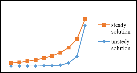
Figure 5. The solution behaviour in the left region, $\bar{\varepsilon}=0.0$
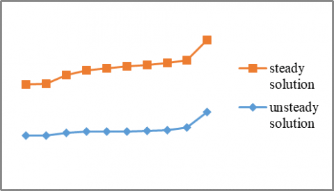
Figure 6. The solution behaviour at the right region, $\bar{\varepsilon}=0.0$
Figure 7. Effect of Rayligh number on the vorticity
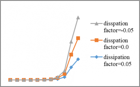
Figure 8. Unsteady solution of temperature in the middle region for different values of dissipation factor
Figure 9. Steady solution of temperature in the middle region fordifferent values of dissipation factor
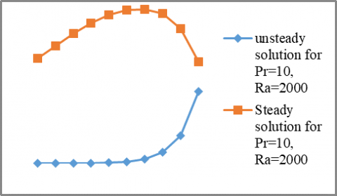
Figure 10. Unsteady vorticity distribution for, $\bar{\varepsilon}=-0.05$, $\mathrm{Ra}=2000, \operatorname{Pr}=100$
Figure 11. Unsteady vorticity distribution for, $\bar{\varepsilon}=-0.05$,$\mathrm{Ra}=2000, \operatorname{Pr}=10$
The authors would like to thank the University of Mosul - IRAQ for the encouragement and support.
[1] Ganish, S. Krishnambal, S. (2007). Unsteady MHD stoks flow of viscous fluid between two parallel porous plates. Journal of Applied Sciences, 7(3): 374-379. https://doi.org/10.3923/jas.2007.374.379
[2] Gnana Prasuna, T., Ramana Murthy, M.V., Venkateswara Rao, G. (2010). Unsteady flow of a viscoelastic fluid through a porous media between two impermeable parallel plates. Journal of Emerging Trends in Engineering and Applied Sciences, 1(2): 225-229.
[3] Attia, H.A., Essawy, M.A.I., Khater, A.H., Ramadan, A.A. (2014). Unsteady non-Darcian flow between two stationery parallel plates in a porous medium with heat transfer subject to uniform suction or injection. Bulgarian Chemical Communications, 46(3): 616-623.
[4] Uwanta, I.J., Hamza, M.M. (2014). Unsteady flow of reactive viscous, heat generating/absorbing fluid with Soret and variable thermal conductivity. International Journal of Chemical Engineering, 2014: 291857. https://doi.org/10.1155/2014/291857
[5] Moses, J.K., Daniel, S., Joseph G.M. (2014). Unsteady MHD cotte flow between two infinite parallel porous plates in inclined magnetic field with heat transfer. International Journal of Mathematics and Statics Invention, 2(3): 103-110.
[6] Hamza, M.M., Usman, I.G., Sule, A. (2015). Unsteady thermodynamic convective flow between two vertical walls in the presence of variable thermal conductivity. Journal of Fluids, 2015: 358053. https://doi.org/10.1155/2015/358053
[7] Uddin, M.J., Rashidi, M.M., Alsulami, H.H., Abbasbandy, S., Freidoonimeh, N. (2016). Two parameters Lie group analysis and numerical solution of unsteady free convective flow of non-Newtonian fluid. Alexandria Engineering Journal, 55(3): 2299-2308. https://doi.org/10.1016/j.aej.2016.05.009
[8] Sattar, A., Subbhni, S.M. (2016). Unsteady MHD flow of a non-newtonian fluid under effect of couple stress between two parallel plates. International Journal for Scientific Research & Development, 4(2): 2321-0613.
[9] Machireddy, G.R., Naramgari, S. (2018). Heat and mass transfer in radiative MHD Carreau fluid with cross diffusion. Ain Shams Engineering Journal, 9(4): 1189-1204. https://doi.org/10.1016/j.asej.2016.06.012
[10] Akhtar, S., Shah, N.A. (2018). Exact solutions for some unsteady flows of a couple stress fluid between parallel plates. Ain Shams Engineering Journal, 9(4): 985-992. https://doi.org/10.1016/j.asej.2016.05.008
[11] Nikodijevic, M., Stamenkovic, Z., Petrovic, J., Kocic, M. (2020). Unsteady fluid flow and heat transfer through a porous medium in a horizontal channel with an inclined magnetic field. Transactions of FAMENA, 44(4): 31-46. https://doi.org/10.21278/TOF.444014420
[12] Islam, T., Parveen, N., Nasrin, R. (2022). Mathematical modeling of unsteady flow with uniform/non-uniform temperature and magnetic intensity in a half-moon shaped domain. Heliyon, 8(3):e09015. https://doi.org/10.1016/j.heliyon.2022.e09015
[13] Hamza, M.M., Shuaibu, A., Kamba, A.S. (2022). Unsteady MHD free convection flow of an exothermic fluid in a convectively heated vertical channel filled with porous medium. Scientific Reports, 12(1): 11989. https://doi.org/10.1038/s41598-022-16064-y
[14] Daidzic, N.E. (2022). Unified theory of unsteady planar laminar flow in the presence of arbitrary pressure gradients and boundary movement. Symmetry, 14(4): 757. https://doi.org/10.3390/sym14040757