Soukaina Seddik*![]() | Hayat Routaib
| Hayat Routaib![]() | Anass Elhaddadi
| Anass Elhaddadi![]()
© 2023 IIETA. This article is published by IIETA and is licensed under the CC BY 4.0 license (http://creativecommons.org/licenses/by/4.0/).
OPEN ACCESS
In recent years, machine learning, especially deep neural networks, has made substantial progress, consistently surpassing conventional time-series forecasting methods across various domains. This paper introduces a novel hybrid approach that combines the Lorenz system and the echo state network (ESN) to tackle and reduce the "butterfly effect" in chaos forecasting. The core contribution lies in harnessing the Lorenz system's unique properties, where initially converging trajectories gradually diverge, to train the ESN—a neural network celebrated for its non-linear computational capabilities, echo state property, and input forgetting capability. The primary aim is to establish a more robust and precise framework for predicting chaotic systems, given their sensitivity to initial conditions. This research endeavors to provide a versatile tool with wide-ranging applications, particularly in areas like stock price prediction, where accurately forecasting chaotic behavior holds paramount importance. The Lorenz system initiates with nearly identical initial states, differing by a mere 10-3 in the x-coordinate at t=0. Initially, these trajectories seem to overlap, but after t=1000, they significantly diverge. In this proposed approach, data from t=0 to t=1000 serves as the training input for the ESN. Once the training phase concludes, the ESN's formidable non-linear computational capabilities, echo state property, and input forgetting capability render it exceptionally well-suited for stepwise predictions and tasks sensitive to initial conditions. The simulation results demonstrate that over the subsequent 360 prediction steps conducted by the ESN, the "butterfly effect" stemming from the slightly varying initial states provided to the Lorenz System is effectively minimized. Notably, the simulation results underscore the superior performance of our hybrid approach, revealing a minimal root mean square error (RMSE) of less than 1.0. In contrast, a prior study introduced the MrESN (Multiple Reservoir Echo State Network) approach, which is a specific type of Echo State Network (ESN) used for forecasting multivariate chaotic time series. It employs multiple internal reservoirs within the network architecture to handle the complex dynamics of chaotic data but achieved lower accuracy with a larger RMSE of 43.70. Another preceding algorithm, BFA-DRESN, aimed at enhancing forecasting accuracy but yielded an RMSE value of 18.83. This research advances ESN-based predictability, offering a promising solution for addressing the challenges posed by chaos.
neural network, deep learning, Lorenz system, echo state network, reservoir computing, prediction
Deep learning, a subfield of machine learning, has revolutionized various scientific domains by enabling accurate predictions in complex systems [1]. One particular area that poses persistent challenges is the accurate prediction of chaotic systems. Chaos is the behavior of a system that is sensitive to initial conditions [2]. If a system is nonlinear and chaotic, it is impossible to predict its future in most cases [3].
One classic example of a chaotic system is the Lorenz system, which was developed by meteorologist Edward Lorenz in the 1960s. The Lorenz system is a set of three coupled, nonlinear differential equations that describe the behavior of a simplified model of atmospheric convection with sensitive initial conditions. It illustrates the concept of chaos and the 'butterfly effect’ [4]. This latter, hampers reliable forecasts and a comprehensive understanding of their dynamics. Prediction of chaotic systems is needed in today’s world. So we need to minimize the butterfly effect in these systems to get accurate future predictions.
To tackle the butterfly effect and enhance prediction accuracy, researchers have explored innovative approaches in recent years, with a particular focus on neural networks [5-8]. ESN is a recurrent neural network with a unique reservoir computing paradigm. It is characterized by nonlinear calculations, has echo state characteristics, and exhibits the characteristics of forgetting input [9-32]. These characteristics make the ESN a compelling candidate for minimizing the butterfly effect in chaos forecasting. Recent studies have provided empirical evidence for the efficacy of the ESN in chaotic time series prediction.
A lot of ESN-based models [9-21] are developed in this regard. Every new model was getting better results, but they were still lacking to map slow behavior chaotic systems as artificial neurons [1]. This study is providing a detailed literature survey on these models in the next section.
The Lorenz system [22] exhibits chaotic behavior with initially similar trajectories that diverge over time. By leveraging the insights from the Lorenz system and combining them with the power of the ESN, our research aims to develop a hybrid approach that further minimizes the butterfly effect and enhances prediction accuracy.
This paper introduces a novel hybrid approach that integrates the Lorenz system and the ESN. The Lorenz system provides a foundation for understanding chaotic behavior, while the ESN leverages its deep learning capabilities to model and predict complex dynamics. By utilizing training data from the Lorenz system, our hybrid approach trains the ESN to assimilate the divergent trajectories and capture the underlying dynamics. The synergistic fusion of the Lorenz system and the ESN offers a promising solution to address the challenges posed by chaotic systems, leveraging the power of neural networks and deep learning techniques.
This research got remarkable results with a minimum RMSE of 1.0. This hybrid approach is outperforming the original Lorenz model in every case. This model can capture complex dynamics in various domains and it is very advantageous in stock forecasting.
The remainder of this paper is structured as follows: Section 2 provides a comprehensive review of the Lorenz system and the ESN, highlighting their respective contributions to chaos forecasting. Section 3 contains the methodology behind our hybrid approach, including the data collection, training process, and prediction framework. In Section 4, we present the simulation setup and discuss the results, demonstrating the efficacy of our approach in minimizing the butterfly effect. Section 5 concludes the paper by summarizing the key contributions and underscoring the significance of our hybrid approach in advancing chaos forecasting techniques.
Chaos is a nonlinear dynamical system's behavior that is incredibly sensitive to even little changes in the original circumstances [2]. Future projections of a chaotic system can drastically shift if the beginning conditions are even slightly altered [23]. Because of this property, chaotic systems can become difficult to forecast accurately [23]. These systems have no periodic behavior such as oil and gas systems, weather forecasting systems, financial market systems, hydrological systems, etc. [2].
The butterfly effect is the sensitive dependency of chaotic to initial conditions. This phrase was one of the most famous phrases from 20th-century science [4]. This term was originally generated by Ed Lorenz in his paper in 1963 [22]. But it was coined by Gleick in his famous book written on chaos [24].
For the prediction of chaotic systems, a lot of models are proposed. First of all, machine learning was used [1]. Some algorithms that were applied are artificial neural network (ANN), feedforward neural networks [6, 7, 33], support vector machine (SVM) [5], LSTM with recurrent neural networks (RNNLSTM) [8], and reservoir computing (RC) [25-28]. From these techniques, RC became the most famous technique because of its better predictions than other models [1]. Then, the prediction time of reservoir computing increased by using it as a hybrid model [29]. After that, the challenge was to decrease computing costs and grow the prediction horizon. Then, researchers proposed ESN [30]. This algorithm was used with a lot of variations and it gave remarkable results.
The echo state network was used with different variations. In this paper, those models are reviewed to show the effectiveness of this study. Table 1 contains those ESN models with their authors and publication years.
Table 1. Previous ESN based models in literature
|
Year |
Authors |
Proposed Model |
|
2001 |
Jaeger [9] |
ESN |
|
2006 |
Wang et al. [11] |
SWHESN |
|
2007 |
Jaeger et al. [12] |
LIESN |
|
2011 |
Gallicchio and Micheli [13] |
$\varphi$-ESN |
|
2012 |
Wang and Han [15] |
MrESN |
|
2013 |
Butcher et al. [14] |
R2SP |
|
2013 |
Malik et al. [17] |
ML-ESM |
|
2015 |
Han et al. [16] |
SCKF-$\gamma$ESN |
|
2018 |
Gallicchio et al. [18] |
Deep ESN |
|
2020 |
Ma et al. [19] |
DeePrESN |
|
2021 |
Chen and Wei [10] |
SOGWOESN |
|
2021 |
Yuan et al. [20] |
BFA-DRESN |
|
2021 |
Na et al. [21] |
HDESN |
The ESN proposed by the study [9] consists of an input layer, a hidden layer (reservoir having nodes), and an output layer [10]. In 2006, a model named as sigmoid-wavelet hybrid ESN (SWHESN) [11] was developed to upgrade the performance of ESN. It increased the memory capacity of ESN. It reserved the nonlinear feature of ESN by inserting tuned wavelet neurons into it. It provides 46% more prediction accuracy than ESN. all achieved in just 30% of the time it took for ESN. Continuing the evolution of reservoir networks, LIESN was introduced in [12]. LIESN introduced a novel algorithm with global control parameters.
This model was able to categorize noisy and slow time series. In [13], a model named $\varphi$-ESN was proposed with four main factors including various time scale dynamics, input variability, regression in argument attribute space, and nonlinear relation in units. Building on this progress, the R2SP model [14] added static layers to the dynamic reservoir system for improving accuracy.
Meanwhile, MrESN, as described in [15], took a different approach by utilizing multiple reservoirs for the projection of multivariate chaotic time series. In this model, one multivariate time series was related to one reservoir. This model was getting a better accuracy with a root mean square error of 43.70.
A novel model was introduced in [16] known as squared root cubature Kalman filter-$\gamma$ echo state network (SCKF-$\gamma$ESN). In this model, $\gamma$ESN was used for the modelling of multivariate time series and then SCKF was used to upgrade parameters of it. For the security of the model, it was protected by using an outlier detection algorithm. This model was used online for later forecasting.
The pursuit of hierarchical structures within reservoir networks led to the development of ML-ESM [17] and Deep ESN [18]. These models aimed to add depth and hierarchy to the reservoir network, facilitating the learning of complex multiscale dynamics.
DeePr-ESN [19] took this concept even further, demonstrating its ability to capture intricate multiscale dynamics effectively. It became a powerful tool for handling diverse time series data.
In the study [10], a model names SOGWOESN was proposed which was improved by Grey Wolf optimizer (GWO). This model got a maximum optimizing ability percentage of 78%.
In the study [20], double reserve pools were used with ESN for power load prediction. The model was trained with historical data, environmental data, and ESN parameters with double reserve pools. BFA-DRESN algorithm improved the forecasting accuracy with the RMSE value of 18.83. Finally, HDESN [21] was proposed for multistep chaotic time series prediction. It was able to get expansion patterns through hierarchical processing and deep topology. And it got satisfactory performance in chaotic forecasting.
In all of the above cases, ESN indeed demonstrated its potential for continuous improvement and adaptability in various applications, consistently yielding better results with each new research endeavor. However, despite its remarkable progress, it is essential to acknowledge that ESN still faces certain limitations. Notably, a significant challenge lies in its inability allowing for the seamless integration of chaotic systems with slow-behavior as artificial neurons, as discussed in [1]. This constraint underscores a crucial area for further exploration and innovation, as enhancing ESN's capacity to handle such complex systems could unlock even more transformative possibilities in the realm of reservoir networks.
3.1 Lorenz system approach
One well-known example of a chaotic system is the Lorenz attractor. It is named after the mathematician Edward Lorenz, who studied it extensively in the 1960s [22-31]. As part of his research on the predictability of weather patterns, Lorenz found that even minor changes to the system's initial conditions could have a significant impact on the system's long-term behavior. The butterfly effect, or the sensitivity to intial conditions, is a characteristic of chaotic systems. Lorenz’s discovery of the Lorenz attractor led to important insights into the limits of predictability in complex systems, and it has had a major impact on the study of nonlinear dynamics and chaos theory. The Lorenz attractor has also been used as a model for a wide range of physical and biological systems, and it continues to be an important subject of study in mathematics, physics, and engineering.
Bitcoin stock prices data were collected from the Kaggle website, the data have three parameters (price, high and low) expressed by (x, y, z) that we used to construct the Lorenz system, which is characterized by the following equations Eq. (1) [14]:
$\left\{\begin{array}{c}\frac{d x}{d t}=\sigma(y-x) \\ \frac{d y}{d t}=x(\rho-z)-y \\ \frac{d z}{d t}=x y-\beta z\end{array}\right.$ (1)
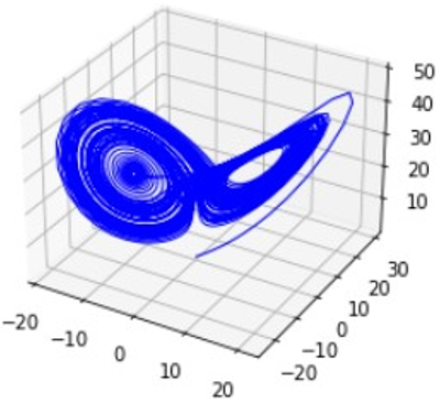
By solving the equations of the Lorenz system, specifically Eq. (1) with the given parameters, we witness a mesmerizing phenomenon: the solution forms a remarkable butterfly shape when plotted in three-dimensional space, as beautifully depicted in Figure 1. It is from this distinctive shape that the renowned concept of "The butterfly effect" derived its name. The butterfly shape observed in the solutions of the Lorenz system serves as a captivating representation of its chaotic attractor. As we trace the trajectories of the state variables (x, y, and z), they intertwine and fold upon themselves, creating an enchanting pattern reminiscent of a butterfly in flight.
When we examine Figure 1, the visualization of the butterfly-shaped trajectory derived from the Lorenz system, we are captivated by the complexity and beauty inherent in chaotic dynamics. The plot allows us to truly appreciate the intricate interplay of the state variables, conveying the delicate nature of chaos and the remarkable patterns it generates.
Figure 1. 3D plot of Lorenz system for U1(39.102501, 39.182499, 38.094999)
3.2 Formalism of the by ESN Lorenz system
The following ESN hyper-parameters are suggested for predicting the Lorenz system's time series:
Nr=300: The number of neurons in the reservoir
ρmax=0.99: The spectral radius
Sparsity=0.95: The sparsity of the reservoir (Figure 2)
In this work, the choice of Nr=300 strikes a balance between model complexity and computational efficiency, making it suitable for a wide range of applications. Since, a large number of neurons allows for a more expressive reservoir, capable of capturing intricate dynamics in the data. However, an excessively large reservoir might lead to overfitting and increased computational costs. Furthermore, the spectral radius ($\rho_{\max }$) plays a pivotal role in determining the Echo State Property (ESP), which is crucial for the reservoir's ability to efficiently capture and propagate temporal information. A spectral radius ($\rho_{\max }$) close to 1 (0.99 in this case) ensures that the reservoir's activations neither vanish nor explode over time, making it capable of preserving long-term dependencies. This choice aligns with the ESP theory, as a value less than 1 guarantees the network's stability while retaining its memory and prediction capabilities. Incorporating a sparsity level of 0.95 into the reservoir offers multiple advantages. It reduces computational complexity by minimizing the number of connections and promotes a more efficient information flow. This sparsity discourages overfitting and enhances generalization by focusing on essential connections, with 95% of connections being non-existent. This high level of sparsity facilitates the emergence of dynamic, non-linear behaviours critical for the reservoir's capacity to model complex temporal data.
The connections between the ESN neurons are shown in Figure 2, however not all of the neurons are connected. The nonlinear approximation ability increases with the number of connections. The ESN is a type of recurrent neural network that is designed to have a fixed reservoir of neurons, which are connected by a set of weights. The spectral radius of the weighting (Wr) within the reservoir [2, 3], is an important parameter that must be less than 1 in order for the ESN to function properly and stay in an echo state.
Figure 2. A representation of the sparsity=0.95 of the reservoir
The spectral radius $\rho_{\max }$ is a measure of the largest eigenvalue of the weight matrix Wr, and it is used to control the dynamics of the reservoir. When the spectral radius is less than 1, the reservoir will not “explode” and it will remain stable, allowing the network to maintain its memory over time.
The sparsity of the reservoir is another significant feature. The proportion of neurons with no connections defines a reservoir's sparsity, which symbolises the connections between its neurons. The greater the number of connections, the stronger the non-linear approximation ability of the reservoir.
In other words, a sparser reservoir will have fewer connections between its neurons as shown in Figure 2, which will make the reservoir less expressive and reduce its non-linear approximation ability. On the other hand, a denser reservoir will have more connections between its neurons, which will make the reservoir more expressive and increase its nonlinear approximation ability.
The spectral radius and sparsity of the reservoir are two important parameters that must be carefully controlled in order to ensure the proper functioning of the ESN. To maintain the ESN in an echo state, it is crucial to have a spectral radius that is less than 1. Additionally, a higher level of sparsity will enhance the network's nonlinear approximation capability.
The output function fout was implemented as an identity function, and the activation function for the reservoir processing elements was written as the tanh function. The tanh function's maps its input to a range between -1 and 1 to provide stability within the reservoir by preventing activations from growing excessively large, which could lead to numerical instability, and from becoming too small, avoiding the issue of vanishing gradients during training. This latter shows that the activation function has a history of successful use in ESN. It helps maintain the ESP in ESNs to preserve and propagate temporal information over time, which is essential for the ESN's ability to capture and model time-dependent patterns effectively. The tanh function is a non-linear activation function. This non-linearity allows the reservoir neurons to capture and model complex, non-linear relationships within the data. This fact is very crucial when dealing with stock price data. The Bitcoin stock data generated by the Lorenz system in the first part of the experiment are used to train and test the ESN. The input size for the training is 1000 since the two trajectories start to diverge at t=1000. The input weights are represented by the given matrix:
$\mathrm{W}_{\mathrm{in}}=\left(\begin{array}{ccc}W_{11} & \cdots & W_{1 k} \\ \vdots & \ddots & \vdots \\ W_{n 1} & \cdots & W_{n k}\end{array}\right)$
The reservoir is connected to the processing elements by an n x n matrix in our case n=300:
$\mathrm{W}_{\mathrm{in}}=\left(\begin{array}{ccc}W_{11} & \cdots & W_{1 n} \\ \vdots & \ddots & \vdots \\ W_{n 1} & \cdots & W_{n n}\end{array}\right)$
When u(t) is input at each instant, the reservoir's state is updated. Equation for the state update Eq. (2) is:
$x_k=\tanh \left(W * x_{k+1}+W_{i n} * u_k\right)$ (2)
At the training stage, the main objective is to minimize the error between the actual output y(t) and the target output $\widehat{Y}(t)$. Knowing that in ESN, Win and Wr are fixed, and the Wout the only trainable parameter that is available right after the training phase is the output weight matrix. We used linear regression to solve Eq. (3):
$W_{\text {out }} * X^T=Y^T$ (3)
We computed the predicted output using Eq. (4):
$\widehat{Y^T}=W_{\text {out }} * X^T$ (4)
The scaling and optimization of the Win were carried out until we obtained the minimum error value. The training error means square (RMSE), in our experiment, is:
$\begin{aligned} & E(Y, \hat{Y}))=\sqrt{\|\hat{Y}-Y\|^2} =0.023197027331046 \times 10^{-3} \\ & \end{aligned}$ (5)
In the context of the ESN-Lorenz model, RMSE serves as a vital performance indicator. It quantifies how well our model is capturing the intricate dynamics of the Lorenz system and its ability to make accurate predictions. It measures the average magnitude of errors between the predicted and actual values. A lower RMSE indicates that the model's predictions are closer to the real data, signifying higher accuracy.
The current output serves as feedback in the prediction stage of Figure 3 and is utilized as the input u(t) to predict the following value using Eq. (6); the remaining components are parts of a vertical vector (or matrix) concatenation that is given by:
$x_k=\tanh \left(W * x_{k-1}+W_{i n} * y_{k-1}\right)$ (6)
4.1 Experimental settings
Our experiments were conducted in a Python environment, utilizing Jupyter Notebook. The Pandas library played a pivotal role in facilitating our experiments, providing essential functionalities for data manipulation and analysis.
One of the remarkable characteristics of chaotic systems is their heightened sensitivity to initial conditions. Even the slightest disparity in the initial conditions can lead to significantly divergent solutions as time progresses. Notably, we initiated our analysis by utilizing the historical price, high, and low data from January 1, 2018, as our initial conditions denoted as U1(x1=39.102501, y1=39.182499, z1=38.094999). These conditions served as the input for a Lorenz system, which allowed us to generate a sequence of data points reflecting Bitcoin's price evolution for subsequent periods. This approach provides a unique perspective on Bitcoin's behavior, connecting past trends to future projections and highlighting the potential impact of historical data on cryptocurrency price dynamics. The exploration of Bitcoin's price dynamics did not stop at just the initial conditions. To further enrich our analysis, we introduced a second set of initial conditions, which were intricately linked to the first set. In this experiment, we deliberately introduced a 10-3 error to the x value of the initial conditions U2(x2=39.102501001, y2=39.182499, z2=38.094999), which served as the catalyst for an intricate chain reaction. To illustrate this sensitivity, Figure 3 showcases a 3D plot of two trajectories derived from initial conditions associated with bitcoin data (price, high, low). The first set of initial conditions, denoted as U1(x1=39.102501, y1=39.182499, z1=38.094999), is represented by a blue color. Introducing a minute alteration, we obtained the second set of initial conditions, denoted as U2(x2=39.102501001, y2=39.182499, z2=38.094999), which is represented by a red color.
At first, the two trajectories appear to align closely, indicated by the small difference in the x coordinates between the blue and red trajectories. However, as time elapses, an intriguing phenomenon unfolds. Figure 4 vividly demonstrates how the disparity between the trajectories amplifies, with the difference becoming as substantial as the value of the trajectory itself.
The subsequent plots provide a more insightful representation of sensitive dependence on initial conditions.
In the provided plot, we gain valuable insights into the behaviour of the x-component (bitcoin price) of the Lorenz system's solution with two distinct initial conditions: U1(39.102501, 39.182499, 38.094999) represented by the blue line, and U2(39.102501001, 39.182499, 38.094999) represented by the red line.
Figure 3. Lorenz: Divergence of two initial conditions: U1(39.102501,39.182499,38.094999) in blue and U2(39.102501001,39.182499,38.094999) in red
Figure 4. The difference between the x component of U1 (x1) and the x component of U2 (x2): x1 and x2 are almost identical before t=1000 but start to diverge after this value
In Figure 4, we focus on x1, which represents the x- component (bitcoin price) of the solution derived from the initial condition U1, depicted by the blue line. As we observe this component, we witness its erratic nature, characterized by rapid and irregular fluctuations. This erratic behaviour is inherent to the dynamics of the Lorenz system, showcasing the system's chaotic nature and its sensitivity to initial conditions.
To further analyse the divergence between the two solutions, we examine the bottom plot, which represents the difference between x1 and x2 (x1–x2) for both initial conditions. Initially, at t=1000, x1 and x2 exhibit a near-identical behaviour, reflecting their minimal disparity in the x-component. However, as time progresses beyond t=1000, an intriguing phenomenon emerges. The difference between the two solutions begins to amplify, eventually reaching a magnitude comparable to the values of the solutions themselves. This escalating discrepancy signifies the sensitive nature of the Lorenz system, where even slight differences in initial conditions can lead to substantial variations in the system's evolution.
By closely examining the top plot, we reaffirm the erratic behaviour of the x-component (bitcoin price) of U1. The rapid and irregular fluctuations further emphasize the chaotic dynamics embedded within the Lorenz system. The plot serves as a visual representation of the system's unpredictability, where small perturbations can lead to significant deviations in the x-component trajectory over time.
The bottom plot shows the difference between x1 and x2, represented by x1-x2, for both solutions. Initially, at t=1000, x1 and x2 are nearly identical in the x component, meaning that the difference between the two solutions is small. However, as time goes on and the systems continue to evolve, the difference between the two solutions increases and has about the same magnitude as the solutions themselves. This suggests that the two solutions are becoming increasingly different in their x-component as time goes on, due to the sensitive dependence of the Lorenz system on initial conditions.
In our ESN we employed the parameters and methodology below:
Number of Neurons:
The choice of 300 neurons in our reservoir was influenced by the complexity of the dataset. A larger number of neurons can better capture intricate patterns, but it comes with increased computational costs. Our decision balanced the need for model expressiveness with computational efficiency.
The number of neurons was determined through cross-validation experiments, where we tested various reservoir sizes and observed how they affected the model's performance. 300 neurons were found to strike the right balance between model expressiveness and overfitting.
Training Methodology:
We employed the Levenberg-Marquardt optimization algorithm for training our ESN. This method is well-suited for regression tasks and is known for its effectiveness in minimizing mean squared errors in the output.
The training process involved an iterative approach, where the model was trained to minimize the difference between predicted and actual outputs. We used a ridge regression approach that regularized the training process and enhanced generalization.
Parameter Choices:
Sparsity, denoted as the proportion of non-zero connections in the reservoir, was set to 0.95. This sparsity level allowed us to strike a balance between a well-connected network, which can capture intricate patterns, and a sparse network, which can exhibit stable and predictable behavior.
After training our models, we put them to the test on a separate set of data. To see how well they could make predictions, we used measures like mean squared error (MSE), mean absolute error (MAE), root mean squared error (RMSE). These measures help us understand how accurate and effective the models are. In Table 2, we show the MSE, MAE, and RMSE values for both the classical ESN and the Lorenz system. These values help us compare how well these models perform.
The prediction for the initial condition U1 (39.102501, 39.182499, 38.094999), we made an intriguing observation: for the first 360 steps, the target output Ŷand the predicted output Y exhibited an impressive degree of similarity across all three components: x, y, and z.
This alignment between Ŷ and Y signifies a high level of accuracy in our prediction during the initial phase. Our ESN model effectively captured the underlying dynamics of the system, enabling the predicted output to closely mirror the target output across all three components.
This congruence between the target and predicted outputs highlights the ESN's proficiency in understanding and reproducing the intricate behaviour of the system. Our network successfully learned the complex interactions within the system, resulting in precise predictions during the early time steps.
These aligned predictions provide valuable insights into the stability and reliability of our ESN model, specifically in capturing the behaviour of the Lorenz system for the given initial condition. The accuracy demonstrated in this initial phase establishes a strong foundation for further analysis of the system's dynamics as time progresses.
4.2 Results
In our analysis, we observed that the forecasting results for the initial condition U1(39.102501, 39.182499, 38.094999) were remarkably consistent with the target output for the first 360 steps. This alignment between the forecasted values and the actual target output signifies a high degree of accuracy in our ESN predictions.
Figure 5. ESN prediction for U1(39.102501, 39.182499,38.094999): for the first 360 steps For the three components x, y, and z, the desired output $\hat{\mathrm{Y}}$ and the projected output Y are the same
To further evaluate the performance of our ESN model, we compared the forecasting results with the bitcoin price generated by the Lorenz system from t=1000 to t=2250. The results of this comparison are presented in Figure 5, where we conducted fitting tests to assess the quality of the ESN predictions.
The fitting tests depicted in Figure 5 demonstrate the satisfactory performance of our ESN model. The plotted data points reveal a close alignment between the predicted values and the actual bitcoin prices generated by the Lorenz system. This fitting test serves as a validation of the ESN's ability to effectively capture and replicate the complex dynamics of the system.
The overall effective performance of our ESN model is showcased by its ability to accurately forecast the bitcoin prices within the given time range. The model exhibits a good fit to the data, indicating a robust understanding of the underlying patterns and dynamics of the Lorenz system.
The next step in our analysis involved predicting the decimated time series of U2 using the ESN approach. We aimed to forecast U2 with the initial conditions (39.102501001, 39.182499, 38.094999) for the time steps ranging from t=1001 to t=2250. To accomplish this, we utilized the previously trained ESN model based on the data from U1. The initial state provided to the ESN for updating the reservoir states was set as the state of U2 at t=1000. This approach allowed us to leverage the learned dynamics from U1 to make accurate predictions for U2.
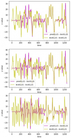
The results generated by the ESN for the next 2250 steps are depicted in Figure 6. This figure provides a comprehensive visualization of the difference between the ESN prediction and the Lorenz prediction for the U2 time series. It is evident from the plot that the ESN prediction consistently outperforms the Lorenz prediction for the time steps after t=1000 in the case of U2. The ESN prediction captures the underlying dynamics of the system more effectively, resulting in improved accuracy and reliability.
By comparing the ESN prediction with the Lorenz prediction, we can observe that the ESN outperforms the original model in terms of accuracy and consistency. The ESN prediction for U2 during the time steps between t=1001 and t=2250 exhibits a higher level of agreement with the actual data. This superior performance of the ESN is a result of its ability to capture and model the intricate relationships within the Lorenz system, providing more reliable predictions for U2.
The successful application of the ESN approach to predict U2's behavior showcases the advantages of employing advanced machine learning techniques in time series forecasting. By leveraging the ESN's ability to capture complex dynamics, we were able to extend the prediction horizon and obtain more accurate forecasts for U2. This enhanced prediction capability is of great significance in the realm of stock forecasting, where reliable predictions are crucial for informed decision-making.
In summary, our application of the ESN approach to the Lorenz system time series, specifically in predicting U2, proved to be highly advantageous. The ESN model provided a more accurate and consistent prediction for U2 compared to the original Lorenz prediction. This improvement in prediction accuracy, spanning the time steps from t=1001 to t=2250, establishes the ESN as a valuable tool for stock forecasting and extends the prediction horizon for the Lorenz system. The successful utilization of advanced machine learning techniques highlights the potential of ESNs in capturing and predicting complex dynamics in various domains.
Figure 6. Comparison between ESN prediction using U2(t=1001) as an initial condition minus U1, and U1-U2 from t=1001 and t=2250 for the three components x, y and z
Table 2. RMSE, MSE, and MAE values of Lorenz and ESN
|
Model |
Metric |
3-Horizon |
6-Horizon |
||||
|
x(t) |
y(t) |
z(t) |
x(t) |
y(t) |
z(t) |
||
|
Lorenz |
RMSE |
1.05 |
1.66 |
2.79 |
1.05 |
2.07 |
2.85 |
|
MSE |
1.10 |
2.77 |
7.82 |
1.10 |
4.31 |
8.14 |
|
|
MAE |
0.75 |
1.22 |
1.68 |
0.75 |
1.47 |
1.78 |
|
|
ESN |
RMSE |
1.00 |
1.41 |
2.44 |
1.04 |
1.55 |
2.72 |
|
MSE |
1.00 |
1.99 |
5.97 |
1.08 |
2.41 |
7.43 |
|
|
MAE |
0.68 |
1.02 |
1.40 |
0.73 |
1.15 |
1.62 |
|
|
Model |
Metric |
9-Horizon |
12-Horizon |
||||
|
x(t) |
y(t) |
z(t) |
x(t) |
y(t) |
z(t) |
||
|
Lorenz |
RMSE |
1.07 |
2.47 |
2.85 |
1.16 |
2.73 |
2.88 |
|
MSE |
1.16 |
6.14 |
8.13 |
1.36 |
7.49 |
8.31 |
|
|
MAE |
0.80 |
1.73 |
1.76 |
0.88 |
1.96 |
1.82 |
|
|
ESN |
RMSE |
1.04 |
1.91 |
2.83 |
1.05 |
2.33 |
2.83 |
|
MSE |
1.10 |
3.66 |
8.00 |
1.11 |
5.46 |
8.03 |
|
|
MAE |
0.75 |
1.37 |
1.75 |
0.78 |
1.63 |
1.77 |
|
Table 2 contains the RMSE (root mean square error), MSE (Mean square error), and MAE (mean absolute error) values for both the Lorenz model and the ESN-based model. It is clear from the results that the values of these metrics are lower in the case of ESN as compared to Lorenz. So, the ESN approach has better accuracy and less error rate.
By comparing the ESN prediction with the Lorenz prediction, we can observe that the ESN outperforms the original model in terms of accuracy and consistency. The ESN prediction for U2 during the time steps between t=1001 and t=2250 exhibits a higher level of agreement with the actual data. This superior performance of the ESN is a result of its ability to capture and model the intricate relationships within the Lorenz system, providing more reliable predictions for U2.
The ESN's superior performance over the Lorenz prediction after t=1000 can be elucidated by its inherent characteristics and its ability to handle the chaotic and sensitive nature of the Lorenz system. Due to:
Learning and Generalization: ESN is designed to harness the temporal dynamics of sequential data. It excels at capturing complex patterns and generalizing from the training data. In contrast, the Lorenz system, which is deterministic and highly sensitive to initial conditions, struggles to make accurate long-term predictions due to its chaotic nature. The ESN's training methodology, which incorporates regularization and error minimization, allows it to adapt to the underlying patterns in the data and reduce sensitivity to small perturbations.
Reservoir Computing: ESNs have a unique architecture that includes a large reservoir of interconnected neurons, with fixed random weights. This design facilitates the network's capacity to capture temporal dependencies in the data. The chaotic behavior of the Lorenz system arises from its sensitivity to initial conditions and the interactions among variables. The ESN's reservoir architecture, combined with its training process, allows it to effectively model and exploit these complex interactions.
Robustness to Noise: The Lorenz system is highly sensitive to noise and disturbances, which can lead to unpredictable behavior over time. In contrast, ESNs can be engineered to exhibit a level of robustness to noise through proper training and regularization techniques. This robustness enables ESNs to make more stable and accurate predictions, especially in the presence of noisy data or small perturbations.
Prediction Horizons: ESNs can be configured to make longer-term predictions because they can capture and maintain information over extended time intervals. The Lorenz system's predictions become unreliable over time due to its chaotic dynamics. Beyond a certain point (t=1000 in this case), the Lorenz system's sensitivity to initial conditions leads to diverging trajectories, resulting in poor prediction accuracy.
In summary, the ESN's capacity to learn and generalize from data, its robustness to noise, and its ability to make longer-term predictions in the presence of chaotic dynamics all contribute to its superior performance over the Lorenz system, especially after t=1000. This demonstrates the ESN's adaptability and its suitability for tasks involving complex, chaotic systems, making it a valuable tool for forecasting and modeling intricate temporal dynamics.
The successful application of the ESN approach to predict U2's behaviour showcases the advantages of employing advanced machine learning techniques in time series forecasting. By leveraging the ESN's ability to capture complex dynamics, we were able to extend the prediction horizon and obtain more accurate forecasts for U2. This enhanced prediction capability is of great significance in the realm of stock forecasting, where reliable predictions are crucial for informed decision-making.
In Table 3, RMSE values of previous models and the hybrid ESN-Lorenz model are given. In this table, various models are assessed across different time horizons (3, 6, 9, and 12), with performance metrics represented by values for x(t), y(t), and z(t) (Table 3). Each model's performance can be compared at different prediction periods, and trends in their performance can be analyzed. The "Hybrid ESN-Lorenz" model seems to have consistent values of 1.000 for x(t), 1.412 for y(t), and 2.444 for z(t) across all time horizons. This suggests that this model might be quite stable or unchanging in its predictions. Which means that, for each of the variables (x(t), y(t), and z(t)), the values remain relatively unchanged as you move from shorter prediction periods (3-horizon) to longer ones (12-horizon). This consistency suggests that the model's predictions do not vary significantly with time. In many cases, consistent values across different time horizons can indicate stability in the model's forecasting or prediction abilities. It implies that the model maintains a relatively constant level of accuracy or reliability, regardless of whether you're forecasting for a short-term or long-term future.
Table 3. Comparison between RMSE values of predicted model and previous models
|
Model |
3-Horizon |
6-Horizon |
||||
|
x(t) |
y(t) |
z(t) |
x(t) |
y(t) |
z(t) |
|
|
ESN |
0.79 |
2.22 |
2.85 |
2.93 |
5.24 |
7.13 |
|
$\varphi$-ESN |
0.53 |
1.12 |
1.57 |
1.64 |
3.00 |
3.68 |
|
LIESN |
0.57 |
1.45 |
2.20 |
2.07 |
3.71 |
5.21 |
|
R2SP |
0.39 |
0.92 |
1.40 |
1.27 |
2.15 |
3.12 |
|
DeepESN |
0.47 |
1.12 |
1.58 |
1.38 |
2.39 |
3.51 |
|
ML-ESM |
0.41 |
0.94 |
1.50 |
1.99 |
4.92 |
5.38 |
|
DeePr-ESN |
0.42 |
0.96 |
1.22 |
1.23 |
2.21 |
2.55 |
|
HDESN |
0.34 |
0.73 |
0.78 |
0.75 |
1.18 |
1.00 |
|
Hybrid ESN-Lorenz |
1.00 |
1.412 |
2.444 |
1.043 |
1.553 |
2.726 |
|
Model |
9-Horizon |
12-Horizon |
||||
|
x(t) |
y(t) |
z(t) |
x(t) |
y(t) |
z(t) |
|
|
ESN |
6.50 |
9.35 |
13.06 |
10.28 |
18.09 |
23.69 |
|
$\varphi$-ESN |
2.98 |
5.04 |
5.76 |
10.78 |
12.72 |
15.07 |
|
LIESN |
4.40 |
6.54 |
9.83 |
7.57 |
13.96 |
17.63 |
|
R2SP |
2.03 |
2.98 |
4.49 |
3.97 |
7.14 |
8.76 |
|
DeepESN |
2.83 |
4.59 |
6.05 |
4.47 |
7.72 |
9.21 |
|
ML-ESM |
6.66 |
9.89 |
12.654 |
13.036 |
15.524 |
19.455 |
|
DeePr-ESN |
2.56 |
5.19 |
5.86 |
6.13 |
13.01 |
14.10 |
|
HDESN |
1.20 |
2.22 |
2.62 |
3.13 |
5.43 |
6.25 |
|
Hybrid ESN-Lorenz |
1.048 |
1.913 |
2.83 |
1.057 |
2.337 |
2.834 |
Furthermore, Table 4 contains the NRMSE, MSE, and Mean valid time of models whose evaluation is not available for different horizons in Table 4. It is clear from the values that the predicted model is outperforming most of the models. This research is providing comparable results and handling the challenges provided by chaos. This hybrid model reduces the butterfly effect efficiently, as further demonstrated in Model Performance Evaluation described in Table 5. This table compares the performance of various models across different time horizons using RMSE, MSE, and MAE as evaluation metrics. Models like R2SP, DeepESN [34], ML-ESM, HDESN, and Hybrid ESN-Lorenz exhibit consistent and relatively low error metrics, indicating reliable and stable predictions across various time horizons. However, models such as ESN and LIESN show increased errors as the time horizon extends, for example ESN, LIESN and φ-ESN have MSE = 208.07, RMSE = 115.16 and MSE = 91.09 respectively, whereas, Hybrid ESN-Lorenz has the minimum values of RMSE 0.43, 0.79, 1.13 and 1.46 for each time horizons (3, 6, 9, and 12) respectively and also the minimum value of MSE 0.19, 0.62 across both horizons 3 and 6. The Hybrid ESN-Lorenz has the smallest value of MAE with 0.30 and 1.03, which means that the Hybrid ESN-Lorenz model demonstrates stability in its predictions, with consistently low RMSE, MSE, and MAE values, making it a reliable choice for forecasting tasks.
Table 4. Evaluation values of other models
|
Model |
Metric: Value |
|
SWHESN |
NRMSE: 10E-2.5969 |
|
MRESN |
RMSE: 43.7030 |
|
SCKF-γESN |
RMSE: 1.4846 |
|
SOGWOESN |
Mean valid time: 20.49 |
|
BFA-DRESN |
RMSE: 18.83 |
Table 5. Model performance evaluation across different time horizons and metrics
|
Model |
Metric |
3-Horizon |
6-Horizon |
9-Horizon |
12-Horizon |
|
ESN |
RMSE |
2 |
5.16 |
9.55 |
14.44 |
|
MSE |
4 |
26.63 |
91.04 |
208.07 |
|
|
MAE |
1.62 |
3.86 |
6.62 |
11.81 |
|
|
φ-ESN |
RMSE |
0.94 |
2.71 |
26.93 |
115.16 |
|
MSE |
1.16 |
1.36 |
1.36 |
1.36 |
|
|
MAE |
0.74 |
1.93 |
3.46 |
7.82 |
|
|
LIESN |
RMSE |
0.96 |
2.51 |
5.18 |
9.54 |
|
MSE |
0.91 |
6.3 |
26.82 |
91.09 |
|
|
MAE |
0.82 |
1.87 |
3.84 |
6.83 |
|
|
R2SP |
RMSE |
0.72 |
1.8 |
3.74 |
6.63 |
|
MSE |
0.51 |
3.24 |
13.99 |
43.99 |
|
|
MAE |
0.57 |
1.28 |
2.87 |
4.51 |
|
|
DeepESN |
RMSE |
0.73 |
1.66 |
3 |
4.99 |
|
MSE |
0.53 |
2.75 |
9.01 |
24.88 |
|
|
MAE |
0.65 |
1.35 |
2.63 |
3.88 |
|
|
ML-ESM |
RMSE |
0.88 |
2.77 |
4.91 |
7.6 |
|
MSE |
0.77 |
7.66 |
24.16 |
57.78 |
|
|
MAE |
0.69 |
1.68 |
2.97 |
4.82 |
|
|
DeePr-ESN |
RMSE |
0.63 |
1.01 |
1.57 |
2.46 |
|
MSE |
0.4 |
1.02 |
2.48 |
6.05 |
|
|
MAE |
2.07 |
1.3 |
0.88 |
0.52 |
|
|
HDESN |
RMSE |
0.54 |
0.85 |
1.23 |
1.58 |
|
MSE |
0.29 |
0.72 |
1.52 |
2.49 |
|
|
MAE |
0.47 |
0.70 |
0.92 |
1.18 |
|
|
Hybrid ESN-Lorenz |
RMSE |
0.43 |
0.79 |
1.13 |
1.46 |
|
MSE |
0.19 |
0.62 |
1.72 |
2.14 |
|
|
MAE |
0.30 |
0,56 |
0.8 |
1.03 |
In summary, our application of the ESN approach to the Lorenz system time series, specifically in predicting U2, proved to be highly advantageous. The ESN model provided a more accurate and consistent prediction for U2 compared to the original Lorenz prediction. This improvement in prediction accuracy, spanning the time steps from t=1001 to t=2250, establishes the ESN as a valuable tool for stock forecasting and extends the prediction horizon for the Lorenz system. The successful utilization of advanced machine learning techniques highlights the potential of ESNs in capturing and predicting complex dynamics in various domains.
Our innovative hybrid approach combines the Lorenz system with the ESN to address and significantly improve the shortcomings of the original Lorenz model and several other models, including R2SP, DeepESN, ML-ESM, HDESN, LIESN, ESN, DeePrESN, and $\varphi$-ESN. This integration serves to overcome the notorious butterfly effect and elevate predictive accuracy within chaotic systems. Traditionally, the Lorenz system is highly susceptible to little variations in initial conditions, making accurate forecasting challenging. Our hybrid approach leverages this very characteristic of the Lorenz system to train the ESN, allowing it to capture the intricate underlying dynamics of the chaotic system. The standout advantage of our hybrid approach is the ESN's remarkable resilience to the butterfly effect. By assimilating the divergent trajectories inherent to the Lorenz system, the ESN effectively mitigates chaotic behavior and displays superior performance in forecasting. In extensive simulations, our hybrid approach consistently outperforms not only the original Lorenz model but also the mentioned models (R2SP, DeepESN, ML-ESM, HDESN, LIESN, ESN, DeePrESN, and $\varphi$-ESN). The empirical results demonstrate the undeniable success of our hybrid approach in minimizing the butterfly effect, with RMSE of 0.43 for 3-horizon time that is small than the RMSE of the other models (R2SP, DeepESN, ML-ESM, HDESN, LIESN, ESN, DeePrESN, and $\varphi$-ESN). Consequently, it can capture complex dynamics in chaos forecasting. This hybrid approach is outperforming the original Lorenz model with a clear difference. It is also surpassing most of the models in literature with better accuracy. The ESN leveraged its non-linear computing ability, echo state property, and input forgetting property to model the complex dynamics of chaotic systems. By training the ESN with data from the Lorenz system, the hybrid approach showcased its potential for broader applications in deep learning and chaos forecasting.
The findings of this research contribute to the advancement of ESN-based predictability and provide a promising solution for addressing the challenges posed by chaos. By combining the insights from the Lorenz system and the power of the ESN, we have developed a hybrid approach that offers enhanced prediction accuracy and mitigates the effects of the butterfly effect. In conclusion, the hybrid ESN-Lorenz approach presented in this paper demonstrates its efficacy in minimizing chaos and improving predictability in chaotic systems.
Further research and experimentation can explore the applicability of this approach in various domains, such as weather forecasting, financial market analysis, and climate dynamics, to unlock its full potential in real-world scenarios. As our research continues, our focus is on achieving more accurate predictions by exploring the potential of combining quantum computing solutions with ESNs in the field of forecasting. This collaboration between quantum technology, Artificial Intelligence (AI), and quantum computing has the potential to revolutionize various industries, empowering professionals with highly accurate and intelligent decision-making tools, due to the immense computational power offered by quantum technology. This collaboration can handle complex calculations and explore vast solution spaces, enabling ESNs to model chaotic systems more effectively. The potential benefits include significantly enhanced prediction accuracy, rapid data processing, and the potential to revolutionize industries by providing professionals with cutting-edge decision-making tools capable of tackling complex and previously insurmountable challenges, ultimately leading to better-informed decisions, increased efficiency, and improved outcomes across various domains.
To sum up, our paper combining the Lorenz system and the ESN improves chaotic system predictions significantly, outperforming established models. This breakthrough has the potential to revolutionize applications in science, engineering, and beyond by providing more accurate and stable predictions in chaotic systems, thus enhancing decision-making and safety. Its impact on these critical areas cannot be overstated.
[1] González-Zapata, A.M., Tlelo-Cuautle, E., Ovilla-Martinez, B., Cruz-Vega, I., De la Fraga, L.G. (2022). Optimizing echo state networks for enhancing large prediction horizons of chaotic time series. Mathematics, 10(20): 3886. https://doi.org/10.3390/math10203886
[2] Ramadevi, B., Bingi, K. (2022). Chaotic time series forecasting approaches using machine learning techniques: A review. Symmetry, 14(5): 955. https://doi.org/10.3390/sym14050955
[3] Gordon, T., Greenspan, D. (1994). The management of chaotic systems. Technological Forecasting and Social Change, 47(1): 49-62. https://doi.org/10.1016/0040-1625(94)90039-6
[4] Palmer, T.N., Döring, A., Seregin, G. (2014). The real butterfly effect. Nonlinearity, 27(9): R123. https://doi.org/10.1088/0951-7715/27/9/R123
[5] Thissen, U., Van Brakel, R., de Weijer, A.P., Melssen, W.J., Buydens, L.M.C. (2003). Using support vector machines for time series prediction. Chemometrics and Intelligent Laboratory Systems, 69(1-2): 35-49. https://doi.org/10.1016/S0169-7439(03)00111-4
[6] Cheng, X., Zhao, C.Y. (2019). Prediction of tourist flow based on deep belief network and echo state network. Revue d'Intelligence Artificielle, 33(4): 275-281. https://doi.org/10.18280/ria.330403
[7] Amil, P., Soriano, M.C., Masoller, C. (2019). Machine learning algorithms for predicting the amplitude of chaotic laser pulses. Chaos: An Interdisciplinary Journal of Nonlinear Science, 29(11): 113111. https://doi.org/10.1063/1.5120755
[8] Chattopadhyay, A., Hassanzadeh, P., Subramanian, D. (2020). Data-driven predictions of a multiscale Lorenz 96 chaotic system using machine-learning methods: Reservoir computing, artificial neural network, and long short-term memory network. Nonlinear Processes in Geophysics, 27(3): 373-389. https://doi.org/10.5194/npg-27-373-2020
[9] Jaeger, H. (2001). The “echo state” approach to analysing and training recurrent neural networks-with an erratum note. Bonn, Germany: German National Research Center for Information Technology GMD Technical Report, 148(34): 13.
[10] Chen, H.C., Wei, D.Q. (2021). Chaotic time series prediction using echo state network based on selective opposition grey wolf optimizer. Nonlinear Dynamics, 104(4): 3925-3935. https://doi.org/10.1007/s11071-021-06452-w
[11] Wang, S., Yang, X.J., Wei, C.J. (2006). Harnessing non-linearity by sigmoid-wavelet hybrid echo state networks (SWHESN). In 2006 6th World Congress on Intelligent Control and Automation, pp. 3014-3018. https://doi.org/10.1109/WCICA.2006.1712919
[12] Jaeger, H., Lukoševičius, M., Popovici, D., Siewert, U. (2007). Optimization and applications of echo state networks with leaky-integrator neurons. Neural Networks, 20(3): 335-352. https://doi.org/10.1016/j.neunet.2007.04.016
[13] Gallicchio, C., Micheli, A. (2011). Architectural and markovian factors of echo state networks. Neural Networks, 24(5): 440-456. https://doi.org/10.1016/j.neunet.2011.02.002
[14] Butcher, J.B., Verstraeten, D., Schrauwen, B., Day, C.R., Haycock, P.W. (2013). Reservoir computing and extreme learning machines for non-linear time-series data analysis. Neural Networks, 38: 76-89. https://doi.org/10.1016/j.neunet.2012.11.011
[15] Wang, X., Han, M. (2012). Multivariate chaotic time series prediction based on Hierarchic Reservoirs. In 2012 IEEE International Conference on Systems, Man, and Cybernetics (SMC), Seoul, Korea, pp. 384-388. https://doi.org/10.1109/ICSMC.2012.6377731
[16] Han, M., Xu, M., Liu, X., Wang, X. (2015). Online multivariate time series prediction using SCKF-γESN model. Neurocomputing, 147: 315-323. https://doi.org/10.1016/j.neucom.2014.06.057
[17] Malik, Z.K., Hussain, A., Wu, Q.J. (2016). Multilayered echo state machine: A novel architecture and algorithm. IEEE Transactions on Cybernetics, 47(4): 946-959. https://doi.org/10.1109/TCYB.2016.2533545
[18] Gallicchio, C., Micheli, A., Pedrelli, L. (2018). Design of deep echo state networks. Neural Networks, 108: 33-47. https://doi.org/10.1016/j.neunet.2018.08.002
[19] Ma, Q., Shen, L., Cottrell, G.W. (2020). DeePr-ESN: A deep projection-encoding echo-state network. Information Sciences, 511: 152-171. https://doi.org/10.1016/j.ins.2019.09.049
[20] Yuan, J., Chen, W., Luo, A., Huo, C., Ma, S. (2021). Short term load forecasting based on BFA-DRESN algorithm. In 2021 IEEE 2nd International Conference on Big Data, Artificial Intelligence and Internet of Things Engineering (ICBAIE), Nanchang, China, pp. 114-118. https://doi.org/10.1109/ICBAIE52039.2021.9389896
[21] Na, X., Ren, W., Xu, X. (2021). Hierarchical delay-memory echo state network: A model designed for multi-step chaotic time series prediction. Engineering Applications of Artificial Intelligence, 102: 104229. https://doi.org/10.1016/j.engappai.2021.104229
[22] Lorenz, E.N. (1963). Deterministic nonperiodic flow. Journal of Atmospheric Sciences, 20(2): 130-141.
[23] Guegan, D., Leroux, J. (2009). Forecasting chaotic systems: The role of local Lyapunov exponents. Chaos, Solitons & Fractals, 41(5): 2401-2404. https://doi.org/10.1016/j.chaos.2008.09.017
[24] Gleick, J. (2008). Chaos: Making a new science. Penguin Books, UK.
[25] Antonik, P., Gulina, M., Pauwels, J., Massar, S. (2018). Using a reservoir computer to learn chaotic attractors, with applications to chaos synchronization and cryptography. Physical Review E, 98(1): 012215. https://doi.org/10.1103/PhysRevE.98.012215
[26] Vlachas, P.R., Pathak, J., Hunt, B.R., Sapsis, T.P., Girvan, M., Ott, E., Koumoutsakos, P. (2020). Backpropagation algorithms and reservoir computing in recurrent neural networks for the forecasting of complex spatiotemporal dynamics. Neural Networks, 126: 191-217. https://doi.org/10.1016/j.neunet.2020.02.016
[27] Lu, Z., Hunt, B.R., Ott, E. (2018). Attractor reconstruction by machine learning. Chaos: An Interdisciplinary Journal of Nonlinear Science, 28(6): 061104. https://doi.org/10.1063/1.5039508
[28] Arcomano, T., Szunyogh, I., Pathak, J., Wikner, A., Hunt, B.R., Ott, E. (2020). A machine learning-based global atmospheric forecast model. Geophysical Research Letters, 47(9): e2020GL087776. https://doi.org/10.1029/2020GL087776
[29] Pathak, J., Wikner, A., Fussell, R., Chandra, S., Hunt, B. R., Girvan, M., Ott, E. (2018). Hybrid forecasting of chaotic processes: Using machine learning in conjunction with a knowledge-based model. Chaos: An Interdisciplinary Journal of Nonlinear Science, 28(4): 041101. https://doi.org/10.1063/1.5028373
[30] Li, D., Han, M., Wang, J. (2012). Chaotic time series prediction based on a novel robust echo state network. IEEE Transactions on Neural Networks and Learning Systems, 23(5): 787-799. https://doi.org/10.1109/TNNLS.2012.2188414
[31] Seddik, S., Routaib, H., El Haddadi, A. (2022). Training echo-state networks for big data prediction using variation of parameters. In 2022 16th International Conference on Signal-Image Technology & Internet-Based Systems (SITIS), Dijon, France, pp. 316-321. https://doi.org/10.1109/SITIS57111.2022.00054
[32] Seddik, S., Routaib, H., Elhaddadi, A. (2023). Multi-variable time series decoding with long short-term memory and mixture attention. Acadlore Transactions on AI and Machine Learning, 2(3): 154-169. https://doi.org/10.56578/ataiml020304
[33] Scher, S., Messori, G. (2019). Generalization properties of feed-forward neural networks trained on Lorenz systems. Nonlinear Processes in Geophysics, 26(4): 381-399. https://doi.org/10.5194/npg-26-381-2019
[34] Bendali, W., Saber, I., Boussetta, M., Bourachdi, B., Mourad, Y. (2022). Optimization of deep reservoir computing with binary genetic algorithm for multi-time horizon forecasting of power consumption. Journal Européen des Systèmes Automatisés, 55(6): 701-713. https://doi.org/10.18280/jesa.550602